Uncertainty Evaluation of Safe Mud Weight Window Utilizing the Reliability Assessment Method

Abstract

Due to the uncertainty of formation properties and improper wellbore stability analysis methods, the input parameters are often uncertain and the required mud weight to prevent wellbore collapse is too large, which might cause an incorrect result. However, the uncertainty evaluation of input parameters and their influence on safe mud weight window (SMWW) is seldom investigated. Therefore, the present paper aims to propose an uncertain evaluation method to evaluate the uncertainty of SMWW. The reliability assessment theory was introduced, and the uncertain SMWW model was proposed by involving the tolerable breakout, the Mogi-Coulomb (MG-C) criterion and the reliability assessment theory. The influence of uncertain parameters on wellbore collapse, wellbore fracture and SMWW were systematically simulated and investigated by utilizing Monte Carlo simulation. Finally, the field observation of well SC-101X was reported and discussed. The results indicated that the MG-C criterion and tolerable breakout is recommended for wellbore stability analysis. The higher the coefficient of variance is, the higher the level of uncertainty is, the larger the impact on SMWW will be, and the higher the risk of well kick, wellbore collapse and fracture will be. The uncertainty of basic parameters has a very significant impact on SMWW, and it cannot be ignored. For well SC-101X, the SMWW predicted by analytical solution is 0.9921–1.6020 g/cm³, compared to the SMWW estimated by the reliability assessment method, the reliability assessment method tends to give a very narrow SMWW of 1.0756–1.0935 g/cm³ and its probability is only 80%, and the field observation for well kick and wellbore fracture verified the analysis results. For narrow SMWW formation drilling, some kinds of advanced technology, such as the underbalanced drilling (UBD), managed pressure drilling (MPD), micro-flow drilling (MFD) and wider the SMWW, can be utilized to maintain drilling safety.

1. Introduction

Due to the exhaustion of conventional petroleum resources, much attention is being paid to some ultra-deep, unconventional and deep-water petroleum resources. To exploit these kinds of petroleum resources, more and more deep wells and ultra-deep wells are utilized [1,2]. The initial deep drilling was just made for petroleum exploration and production, but now is being applied to exploit deep geothermal energy and geo-resources, and to conduct international continental scientific drilling [1]. The initial oil well was only drilled to a depth of 19.8 m, while current oil wells can be drilled to more than 10,000 m, and the deepest well is the SG-3 well that was drilled to a depth of 12,262 m on the Kola Peninsula in Russia in 1984. Currently, most oil wells can be drilled deeper than 6000–8000 m. Deep and ultra-deep drilling usually encounters some challenges, such as the high-temperature and high-pressure (HTHP), wellbore collapse, wellbore fracture, lost circulation, gas kick, and blowout [1]. The reasons may be the uncertainty of formation pressure, the uncertainty of formation lithology, the uncertainty of the reservoir interface depth, the uncertainty of completion depth, and the interaction of multiple factors. In order to minimize or avoid the above challenges that encountered in deep and ultra-deep drilling, drilling engineers need to keep the wellbore pressure within a safe window. If the safe window is converted to the equivalent density, the safe window can be called a safe mud weight window (SMWW). The design of mud weight should follow the following principle: the safe mud weight should be higher than the lowest safe mud weight and lower than the highest safe mud weight. In general, the lowest safe mud weight depends on the minimum between the pore pressure and collapse pressure, while the highest safe mud weight depends on the fracture pressure [3,4,5]. The important foundation of SMWW should be determined by wellbore stability. The wellbore instability, a classical rock mechanics problem, is one of the most complex problems that encountered during drilling and completion, which cost the drilling industry certainly more than $100 million per year worldwide [5,6]. Wellbore instability is recognized when the hole diameter is markedly different from the bit size and the hole does not maintain its structural integrity [3]. In general, the mechanical failure occurs when wellbore stress concentrations exceed the rock strength, and the mechanical failure of wellbore can be classified into two main types (Figure 1): (1) Compressive failure, i.e., “tight hole” or “stuck pipe” incidents, which are time-consuming to solve and therefore expensive, an increased borehole diameter will occur due to brittle failure and the subsequent caving of the wellbore wall in brittle rocks, a reduced borehole diameter which occurs in weak (plastic) shales, sandstones, and salts; and (2) Tensile failure, i.e., “lost circulation” or “mud loss” problems, which are potentially dangerous, thus representing a safety risk that has to be avoided.

In order to investigate the wellbore stability, a large number of analysis methods has been proposed, such as the elastic model, plastic model, elastoplastic model, poro-elastic model, thermo-poro-elastic model, chemo-poro-elastic model and chemo-thermo-poro-elastic model [2,3,4,5,6,7,8,9,10,11,12,13]. However, due to the uncertainty of formation lithology, the uncertainty of formation pressure, the uncertainty of mechanical properties of rocks, and the unstable wellbore pressure, the input parameters of wellbore stability analysis never can be known precisely. In other words, the input parameters are often uncertain, which might cause an incorrect result [14,15,16,17,18,19,20,21,22,23,24,25,26,27,28,29,30]. In order to quantify the influence of uncertain parameters on wellbore stability and SMWW, it’s necessary to utilize reliability assessment method. Morita [14] conducted an uncertainty analysis of borehole stability based on a statistical error analysis method. McLellan and Hawkes [15] indicated that the traditional models fail to account for the inherent variability of rock properties, as well as uncertain values for input parameters, a probabilistic technique was used to evaluate the risks of borehole instability or sand production, and a spreadsheet-based Monte Carlo simulation tool was involved. Ottesen et al. [16] present a new analysis method of wellbore stability based on the quantitative risk analysis (QRA) principles. De Fontoura [17] investigated three analytical methods for evaluating the influence of parameter uncertainties on wellbore stability, such as the first order second moment, first order reliability model and statistical error analysis method, and contrasted with the results generated by Monte Carlo method. Moos et al. [18] and Zoback [6] presented the use of QRA to formally account for the uncertainty in each input parameter to assess the probability of achieving a desired degree of wellbore stability at a given mud weight. Sheng et al. [19] indicated that because of uncertainty in some key influential parameters, these can lead to uncertainty of wellbore stability, a Monte Carlo uncertainty analysis technique was combined with a numerical geomechanical modelling method to develop a geostatistical approach to determine the uncertainty of wellbore stability. Al-Ajmi and Al-Harthy [20] calculated the value of drilling fluid pressure as a probability distribution by utilizing a probabilistic approach captures uncertainty in input variables through running a Monte Carlo simulation. Aadnøy [21], Aadnoy and Looyeh [4] also utilized QRA to assess the effects of the errors or uncertainties associated with the key data on the instability analysis. Zhang et al. [22] deduced a reliability calculation formula for collapse pressure in coal seam drilling by integration of the reliability theory and the Hoek-Brown criterion, and the Weibull distribution and Monte Carlo simulation was utilized in this study. Udegbunam et al. [23] investigated typical fracture and collapse models with respect to inaccuracies in the input data with a stochastic method. Kinik et al. [24,25] presented a mathematical model to estimate the true fracture pressure from the leak-off-test data, and the QRA was also involved to represent the probability-density distribution of fracture pressure. Gholami et al. [26] applied the QRA to consider the uncertainty of input parameters in determining of the mud weight window for different failure criteria, such as the Mohr-Coulomb (M-C), Hoek-Brown (H-B) and Mogi-Coulomb (MG-C) criterion. Plazas et al. [27] investigated a stochastic approach along with the conventional wellbore stability analysis enables to take into account uncertainty from input data.

Although the reliability assessment method had been integrated with wellbore stability models, but most of the above studies still have some shortcomings: (1) The required mud weight to prevent wellbore collapse is too high [28,29], due to the fact traditional wellbore stability models assume that the critical failure appears at the highest point of stress concentration, in other words, it’s performed to yield no shear failure along the borehole wall [2,28]. In real drilling engineering, a tolerable breakout or an appropriate breakout width will not cause an unbearable collapse problem, and it can help lower the required mud weight to prevent collapse; once a tolerable breakout or an appropriate breakout width was involved, the SMWW can be therefore widened, and it’s beneficial to the narrow SMWW formations. However, most of the above studies did not involve a tolerable breakout or an appropriate breakout width, only Morita [14] and Aadnoy and Looyeh [4] investigated its influence on wellbore collapse. (2) Most of wellbore stability analysis that involved the reliability assessment method always uses the M-C criterion to determine the shear failure, while the M-C criterion ignored the influence of the intermediate principal stress, which makes the required mud weight to prevent wellbore collapse too conservative. Al-Ajmi and Zimmerman [7,8] introduced an analytical solution of collapse pressure in conjunction with a true triaxial criterion, i.e., the MG-C criterion, it overcomes the above defect. (3) Most of the above studies just focus on the uncertainty evaluation of wellbore collapse, and the uncertainty evaluation of SMWW is seldom investigated, and the influences of uncertain basic parameters on SMWW are also seldom investigated. Therefore, this study takes the tolerable breakout and the MG-C criterion into account to determine the required SMWW by using the reliability assessment method. Firstly, the basic principle of reliability assessment theory was introduced briefly. Secondly, the uncertain SMWW model was proposed by involving the tolerable breakout, the MG-C criterion and the reliability assessment method. Thirdly, the uncertainty of input parameters was investigated, and the uncertainty analysis of the equivalent mud weight of collapse pressure (EMWCP), the equivalent mud weight of fracture pressure (EMWFP), the equivalent mud weight of collapse pressure (EMWPP) and the SMWW were investigated. Finally, the field observation of well SC-101X was reported and discussed.

2. Reliability Assessment Theory

Reliability calculations provide a means of evaluating the combined effects of uncertainties, and a means of distinguishing between conditions where uncertainties are particularly high or low [29]. “Reliability” as it is used in reliability theory is the probability of an event occurring or the probability of a “positive outcome”. Based on the theory of reliability assessment, we can sort the influencing factors into two types: (1) Loads Q, and (2) Resistances R [30]. The SMWW assessment needs to consider the influence of well kick, wellbore collapse, and wellbore fracture:

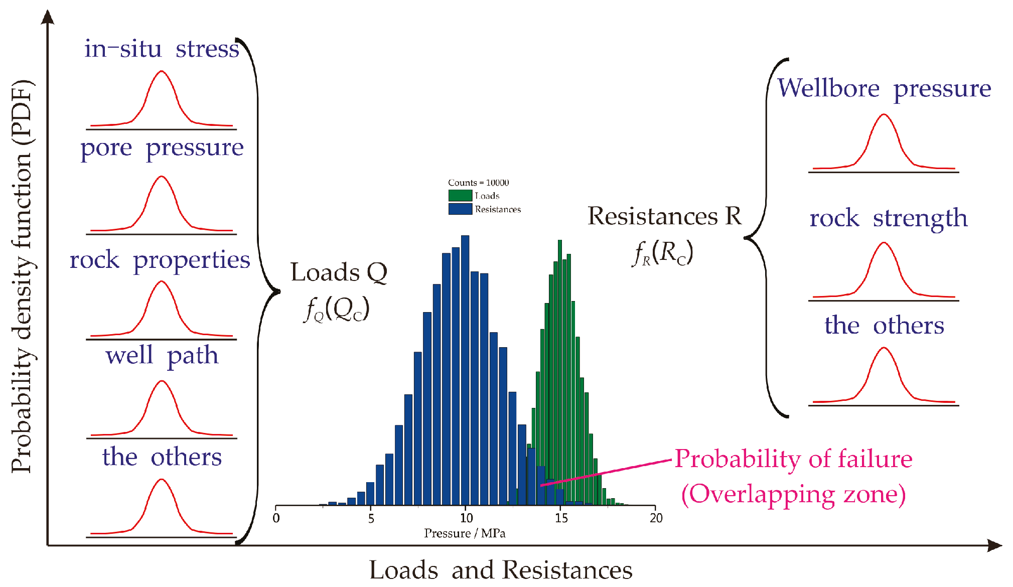
• For well kick, the loads Q denotes the pore pressure, while the resistances R denotes the wellbore pressure; and the basic random variables of loads and resistances of well control can be assumed as ${\mathit{X}}_{\mathrm{QK}}=\{X_{\mathrm{QK}1},X_{\mathrm{RK}2},\cdots ,X_{\mathrm{QK}n}\}$, ${\mathit{X}}_{\mathrm{RK}}=\{X_{\mathrm{RK}1},X_{\mathrm{RK}2},\cdots ,X_{\mathrm{RK}n}\}$.
• For wellbore collapse, the loads Q denotes the collapse pressure that controlled by in-situ stress, pore pressure and rock properties; while the resistances R denotes the wellbore pressure and rock strength; and the basic random variables of loads and resistances of wellbore collapse can be assumed as ${\mathit{X}}_{\mathrm{QC}}=\{X_{\mathrm{QC}1},X_{\mathrm{RC}2},\cdots ,X_{\mathrm{QC}n}\}$, ${\mathit{X}}_{\mathrm{RC}}=\{X_{\mathrm{RC}1},X_{\mathrm{RC}2},\cdots ,X_{\mathrm{RC}n}\}$.
• For wellbore fracture, the loads Q denotes the wellbore pressure; while the resistances R denotes the collapse pressure that controlled by in-situ stress, pore pressure, rock properties and rock strength; and the basic random variables of loads and resistances of wellbore fracture can be assumed as ${\mathit{X}}_{\mathrm{QF}}=\{X_{\mathrm{QF}1},X_{\mathrm{RF}2},\cdots ,X_{\mathrm{QF}n}\}$, ${\mathit{X}}_{\mathrm{RF}}=\{X_{\mathrm{RF}1},X_{\mathrm{RF}2},\cdots ,X_{\mathrm{RF}n}\}$.

The loads and resistances can be assumed as:

$$\{\begin{array}{l}{Q}_k=Q\left({\mathit{X}}_{\mathrm{Q}k}\right)=Q\left(X_{\mathrm{Q}k1},X_{\mathrm{R}k2},\cdots ,X_{\mathrm{Q}kn}\right)\\ R_k=R\left({\mathit{X}}_{\mathrm{R}k}\right)=R\left(X_{\mathrm{R}k1},X_{\mathrm{R}k2},\cdots ,X_{\mathrm{R}kn}\right)\end{array}$$

(1)

where Q_k and R_k are the loads and resistances; k denotes the subscript, k can value for K, C and F for well kick, wellbore collapse, and wellbore fracture, respectively.

The margin of safety, M, is the difference between the resistance and the load. The margin of safety for well control, wellbore collapse and wellbore fracture can be expressed as [30,31]:

$$M_k=R_k-Q_k$$

(2)

where M_k is the margin of safety for factor k.

In general, the loads and resistances are two independent random variables, and the reliability and failure probability can be expressed as [30,31]:

$$P_{rk}=P\left(M_k>0\right)=P\left[\left(R_k-Q_k\right)>0\right]$$

(3)

$$P_{fk}=P\left(M_k<0\right)=P\left[\left(R_k-Q_k\right)<0\right]$$

(4)

where P_rk is the reliability of factor k; P_fk is the failure probability of factor k.

There is a relationship between the reliability and failure probability:

$$P_{rk}+P_{fk}=1$$

(5)

If we assume that the probability density function of Q_k and R_k are f_Q(Q_k) and f_R(R_k), respectively. Figure 2 shows the interference of the probability density function of Q_k and R_k, we just take the assessment of wellbore collapse as an example, the well control and wellbore fracture is similar. The overlapping zone denotes the probability of failure. The smaller overlapping zone, the wellbore will be more reliable, i.e., the risk of wellbore collapse will be lower; the bigger overlapping zone, the wellbore will be more unreliable, i.e., the risk of wellbore collapse will be higher. The reliability and failure probability can be expressed as [31]:

$$\{\begin{array}{l}{P}_{rk}=P\left(M_k>0\right)={\displaystyle {\int }_0^{\infty }f(M_k)d{M}_k}={\displaystyle {\int }_0^{\infty }{\displaystyle {\int }_0^{\infty }{f}_Q(M_k+Q_k)f_R(R_k)d{R}_{k}d{M}_k}}\\ P_{fk}=P\left(M_k<0\right)={\displaystyle {\int }_{-\infty }^{0}f(M_k)d{M}_k}={\displaystyle {\int }_{-\infty }^0{\displaystyle {\int }_{-M_k}^{\infty }{f}_Q(M_k+Q_k)f_R(R_k)d{R}_{k}d{M}_k}}\end{array}$$

(6)

where f_Q(Q_k) and f_R(R_k) are the probability density function of Q_k and R_k, respectively.

3. Modeling for Safe Mud Weight Window Utilizing Reliability Assessment

3.1. Stress Distribution on the Borehole Wall

In order to determine the stress distribution on the wall of the vertical borehole, several basic assumptions are made to propose this model [3,4,5]: (1) The material of deep formation is linear elastic, homogeneous and isotropic; (2) The mechanical model can be simplified as a plane-strain problem; (3) The formation rock obeys the small deformation assumption; (4) In-situ stress state (σ_H, σ_h, σ_v), pore pressure (p_p), strength parameters (c, φ) and material parameters (v) are known. Based on the stress distribution around the wellbore, and considering the effects of flow induced stress, the stress components on the wall of the borehole (r = R) can be expressed as [5]:

$$\{\begin{array}{l}{\sigma }_r=p_m\\ {\sigma }_{\theta }=-p_m+\left(1-2\cos 2\theta \right){\sigma }_H+\left(1+2\cos 2\theta \right){\sigma }_h\\ {\sigma }_z={\sigma }_v-2v\left({\sigma }_H-{\sigma }_h\right)\cos 2\theta \end{array}$$

(7)

where σ_v, σ_H and σ_h are the vertical, maximum and minimum horizontal in-situ stresses respectively, MPa; p_m is the wellbore pressure, MPa; v is the Poisson’s ratio; θ is the angle of circumference, (°); σ_r, σ_θ and σ_z are the stress components on the borehole wall, MPa.

For a vertical well, according to the Equation (1), tangential stress (σ_θ) and axial stress (σ_z) are functions of the angle θ, and the tangential and axial stresses will vary sinusoidally, as shown in Figure 3. Both tangential and axial stresses reach the highest magnitude when θ = π/2 or 3π/2, i.e., θ_max = π/2 or 3π/2.

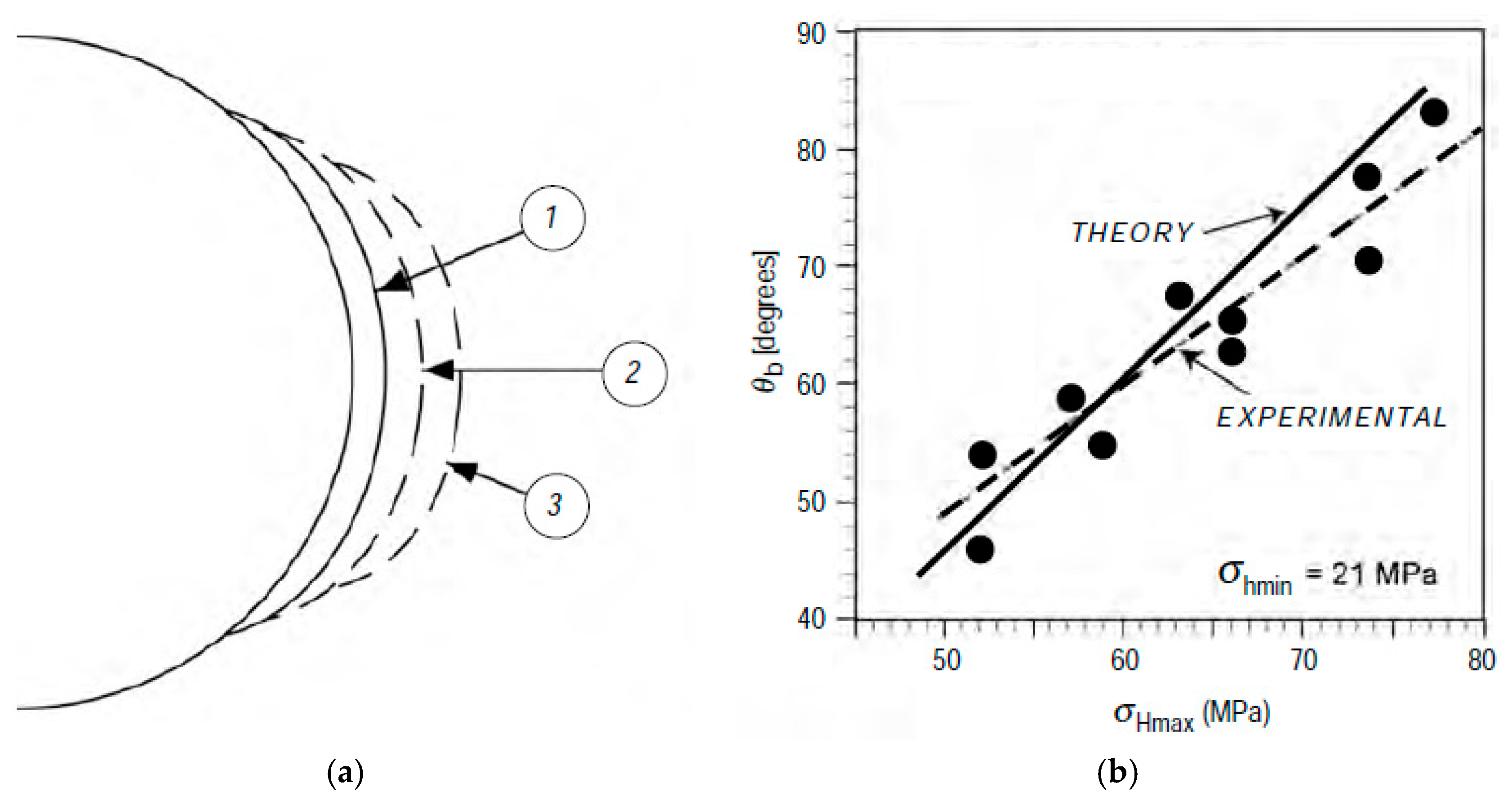
3.2. Breakout Width Model

As shown in Figure 4, the traditional method predicts the collapse pressure using the critical failure point, and the critical failure point is located at the point A:

$${\theta }_c={\theta }_{\max }=0.5\pi \mathrm{or}{\theta }_c={\theta }_{\max }=1.5\pi$$

(8)

where θ_c is the angle of critical failure point B, (°); θ_max the angle of critical failure point A, (°).

However, the breakout width model assumes a tolerable breakout width (2ω) to calculate the collapse pressure, i.e., the critical failure point occurs at the point B [2,28]:

$${\theta }_c={\theta }_{\max }\pm \omega =0.5\pi \pm \omega \mathrm{or}{\theta }_c={\theta }_{\max }\pm \omega =1.5\pi \pm \omega$$

(9)

where ω is the half of the tolerable breakout width, (°).

In general, the breakout occurs as a series of successive spalls along the direction of the minimum principal horizontal stress and results from shear failure subparallel to the free wall of the borehole [2,6,28,32,33,34,35,36,37]. As shown in Figure 5, where ①, ② and ③ represent the breakout zones during deepening. For a tolerable breakout, the wellbore collapse accident could not happen, because the borehole will form a stable shape after several breakouts. In general, when the breakout width does not exceed a tolerable value, the wellbore breakouts are usually expected to increase in depth, but not in width, resulting in a stable borehole after several breakouts [2,6]. The measured breakout widths also compared very well with those predicted by the simple theory [6]. Thus, the given point B (θ_c = θ_max ± ω) can be replaced by the traditional critical failure point A to calculate the collapse pressure for a given tolerable breakout. Zoback [6] indicated that the tolerable breakout width (2ω) to prevent borehole collapse can be set as 90° for a vertical borehole. Once the breakout width (2ω) exceeds the allowable breakout width, the borehole cannot maintain its stability.

Substituting Equation (9) into Equation (7), the stress components of the critical failure point B can be rewritten as:

$$\{\begin{array}{l}{\sigma }_r=p_m\\ {\sigma }_{\theta }=-p_m+\left[1-2\cos 2\left({\theta }_{\max }+\omega \right)\right]{\sigma }_H+\left[1+2\cos 2\left({\theta }_{\max }+\omega \right)\right]{\sigma }_h\\ {\sigma }_z={\sigma }_v-2v\left({\sigma }_H-{\sigma }_h\right)\cos 2\left({\theta }_{\max }+\omega \right)\end{array}$$

(10)

3.3. Collaspe Pressure Model for M-C Criterion

3.3.1. M-C Criterion

If considering the conventional effective stress concept, the detail derivation process of the M-C criterion can refer to Appendix A, and it can be expressed as [7]:

$${\sigma }_1=C+q{\sigma }_3$$

(11)

where C and q are given as:

$$\{\begin{array}{l}C=\frac{2c\cos \phi }{1-\sin \phi }-\left(q-1\right)\alpha p_p\\ q=\frac{1+\sin \phi }{1-\sin \phi }\end{array}$$

(12)

where φ is the friction angle, (°); c is the cohesive strength, MPa; σ₁ and σ₃ are the major and minor principal stress, MPa; α is the Biot’s coefficient; p_p is the pore pressure, MPa.

3.3.2. Collapse Pressure

According to Equation (7), the radial stress is perpendicular to the borehole wall, i.e., it’s a principal stress. In these models there are three permutations of the three principal stresses that need to be investigated in order to determine the required mud pressure [19]: (1) σ_z ≥ σ_θ ≥ σ_r, (2) σ_θ ≥ σ_z ≥ σ_r, and (3) σ_θ ≥ σ_r ≥ σ_z. In the fields, the case where σ_θ ≥ σ_z ≥ σ_r is the most commonly encountered stress state corresponding to borehole collapse [19]. Substituting σ₁ = σ_θ, σ₂ = σ_z and σ₃ = σ_r into Equations (11) and (12), the collapse pressure model with a tolerable breakout width can be expressed as:

$$p_c=\frac{\left[1-2\cos 2\left({\theta }_{\max }+\omega \right)\right]{\sigma }_H+\left[1+2\cos 2\left({\theta }_{\max }+\omega \right)\right]{\sigma }_h-C}{1+q}$$

(13)

where p_c is the collapse pressure, MPa.

If set the critical failure point θ_c = θ_max ± ω =π/2 or 3π/2, Equation (13) can be reduced to the traditional model:

$$p_c=\frac{3{\sigma }_H-{\sigma }_h-C}{1+q}$$

(14)

3.3.3. Equivalent Mud Weight of Collapse Pressure (EMWCP)

The collapse pressure (p_c) can be predicted by using Equation (13) or Equation (14), and the equivalent mud weight (EMW) of collapse pressure (EMWCP) can be expressed as:

$$\mathrm{EMWCP}=\frac{p_c}{gTVD}$$

(15)

where EMWCP is the equivalent mud weight of collapse pressure, g/cm³; g is the gravitational acceleration, g = 9.8 m/s²; TVD is the true vertical depth, km.

According to Equations (13)–(15), the true vertical depth (TVD), the gravitational acceleration (g) and the critical failure point A (θ_max) are usually certain, while the maximum horizontal stress (σ_H), minimum horizontal stress (σ_h), tolerable breakout width (ω), pore pressure (p_p), strength parameters (c, φ) and Biot’s coefficient (α) are usually uncertain. The basic random variables of loads and resistances of wellbore collapse can be expressed as:

$$\{\begin{array}{l}{\mathit{X}}_{\mathrm{QC}}=\{{\sigma }_H,{\sigma }_h,p_p,\alpha ,\omega \}\\ {\mathit{X}}_{\mathrm{RC}}=\{c,\phi ,p_m\}\end{array}$$

(16)

The loads and resistances of wellbore collapse can be expressed as:

$$\{\begin{array}{l}{Q}_{\mathrm{C}}=\mathrm{EMWCP}=Q({\mathit{X}}_{\mathrm{QC}})=Q\left({\sigma }_H,{\sigma }_h,p_p,\alpha ,\omega \right)\\ R_{\mathrm{C}}=\mathrm{EMWWP}=R({\mathit{X}}_{\mathrm{RC}})=R\left(c,\phi ,p_m\right)\end{array}$$

(17)

Substituting Equations (13)–(16) into Equation (17), the reliability and failure probability can be determined by using the reliability assessment theory.

3.4. Collaspe Pressure Model for MG-C Criterion

3.4.1. MG-C Criterion

If considering the conventional effective stress concept, the detail derivation process of the MG-C criterion can refer to Appendix B, and the MG-C criterion can be expressed as [2,7]:

$${\left(I_1^2-3I_2\right)}^{\frac{1}{2}}=a^{\prime }+b^{\prime }\left(I_1-{\sigma }_2-2\alpha p_p\right)$$

(18)

where I₁, I₂, a′ and b′ are given as:

$$\{\begin{array}{l}{I}_1={\sigma }_1+{\sigma }_2+{\sigma }_3\\ I_2={\sigma }_1{\sigma }_2+{\sigma }_2{\sigma }_3+{\sigma }_3{\sigma }_1\end{array}$$

(19)

$$\{\begin{array}{l}{a}^{\prime }=2c\cos \phi \\ b^{\prime }=\sin \phi \end{array}$$

(20)

where σ₂ is the intermediate principal stress, MPa; I₁ is the first stress tensor invariant, MPa; I₂ is the second stress tensor invariant, MPa.

3.4.2. Collapse Pressure

According to Equation (7), the radial stress is perpendicular to the borehole wall, i.e., it’s a principal stress. In these models there are three permutations of the three principal stresses that need to be investigated in order to determine the required mud pressure [19]: (1) σ_z ≥ σ_θ ≥ σ_r, (2) σ_θ ≥ σ_z ≥ σ_r, and (3) σ_θ ≥ σ_r ≥ σ_z. In the fields, the case where σ_θ ≥ σ_z ≥ σ_r is the most commonly encountered stress state corresponding to borehole collapse [19]. Substituting σ₁ = σ_θ, σ₂ = σ_z and σ₃ = σ_r into Equations (18)–(20), the collapse pressure model with a tolerable breakout width can be expressed as:

$$p_c=\frac{1}{2}A-\frac{1}{6}{\left\{12{\left[a^{\prime }+b^{\prime }\left(A-2\alpha p_p\right)\right]}^2-3{\left(A-2B\right)}^2\right\}}^{\frac{1}{2}}$$

(21)

where A, B, a′ and b′ are given as:

$$\{\begin{array}{l}A=\left[1-2\cos 2\left({\theta }_{\max }+\omega \right)\right]{\sigma }_H+\left[1+2\cos 2\left({\theta }_{\max }+\omega \right)\right]{\sigma }_h\\ B={\sigma }_v-2v\left({\sigma }_H-{\sigma }_h\right)\cos 2\left({\theta }_{\max }+\omega \right)\end{array}$$

(22)

$$\{\begin{array}{l}{a}^{\prime }=2c\cos \phi \\ b^{\prime }=\sin \phi \end{array}$$

(23)

If set the critical failure point θ′ = θ_max ± ω = π/2 or 3π/2, substituting θ′ = θ_max ± ω = π/2 or 3π/2 into Equation (22), the collapse pressure model can degrade into the traditional model:

$$\{\begin{array}{l}A=3{\sigma }_H-{\sigma }_h\\ B={\sigma }_v+2v\left({\sigma }_H-{\sigma }_h\right)\end{array}$$

(24)

3.4.3. Equivalent Mud Weight of Collapse Pressure (EMWCP)

The collapse pressure (p_c) can be predicted by using Equation (21), and the EMWCP can be expressed as:

$$\mathrm{EMWCP}=\frac{p_c}{gTVD}$$

(25)

According to Equations (21)–(25), the TVD, the gravitational acceleration (g) and the critical failure point A (θ_max) are usually certain, while the vertical stress (σ_v), maximum horizontal stress (σ_H), minimum horizontal stress (σ_h), Poisson’s ratio (v), tolerable breakout width (ω), pore pressure (p_p), strength parameters (c, φ) and Biot’s coefficient (α) are usually uncertain. The basic random variables of loads and resistances of wellbore collapse can be expressed as:

$$\{\begin{array}{l}{\mathit{X}}_{\mathrm{QC}}=\{{\sigma }_H,{\sigma }_h,{\sigma }_v,p_p,v,\alpha ,\omega \}\\ {\mathit{X}}_{\mathrm{RC}}=\{c,\phi ,p_m\}\end{array}$$

(26)

The loads and resistances of wellbore collapse can be obtained:

$$\{\begin{array}{l}{Q}_{\mathrm{C}}=\mathrm{EMWCP}=Q({\mathit{X}}_{\mathrm{QC}})=Q\left({\sigma }_H,{\sigma }_h,{\sigma }_v,p_p,v,\alpha ,\omega \right)\\ R_{\mathrm{C}}=\mathrm{EMWWP}=R({\mathit{X}}_{\mathrm{RC}})=R\left(c,\phi ,p_m\right)\end{array}$$

(27)

Substituting Equations (21)–(26) into Equation (27), the reliability and failure probability can be determined by using the reliability assessment theory.

3.5. Facture Pressure Model

3.5.1. Tensile Failure Criterion

When the tensile stress exceeds the tensile strength, the wellbore fracture will occur. In general, the maximum tensile stress criterion can be used to determine the wellbore fracture. If considering the conventional effective stress concept, the tensile failure criterion can be written as:

$${\sigma }_3-\alpha p_p+S_t=0$$

(28)

where S_t is the tensile strength, in MPa.

3.5.2. Facture Pressure

According to Equation (10), only the hoop stress can obtain the negative value, and the minor principal stress (σ₃) occurs at θ = 0° or 180°. Substituting θ = 0° or 180° into Equation (10), the minor principal stress (σ₃) can be expressed as:

$${\sigma }_3=3{\sigma }_h-{\sigma }_H-p_m-\alpha p_p$$

(29)

Substituting Equation (29) into Equation (28), the fracture pressure model can be obtained:

$$p_f=3{\sigma }_h-{\sigma }_H-\alpha p_p+S_t$$

(30)

where p_f is the fracture pressure, MPa.

3.5.3. Equivalent Mud Weight of Fracture Pressure (EMWFP)

The fracture pressure (p_f) can be predicted by using Equation (30), and the EMW of fracture pressure (EMWFP) can be expressed as:

$$\mathrm{EMWFP}=\frac{p_f}{gTVD}$$

(31)

where EMWFP is the equivalent mud weight of fracture pressure, g/cm³.

According to Equations (30) and (31), the TVD and the gravitational acceleration (g) are usually certain, while the maximum horizontal stress (σ_H), minimum horizontal stress (σ_h), pore pressure (p_p), strength parameters (S_t) and Biot’s coefficient (α) are usually uncertain. The basic random variables of loads and resistances of wellbore fracture can be expressed as:

$$\{\begin{array}{l}{\mathit{X}}_{\mathrm{QF}}=\left\{p_m\right\}\\ {\mathit{X}}_{\mathrm{RF}}=\{{\sigma }_H,{\sigma }_h,p_p,S_t,\alpha \}\end{array}$$

(32)

The loads and resistances of wellbore fracture can be obatined:

$$\{\begin{array}{l}{Q}_{\mathrm{C}}=\mathrm{EMWWP}=Q({\mathit{X}}_{\mathrm{QF}})=Q\left(p_m\right)\\ R_{\mathrm{C}}=\mathrm{EMWFP}=R({\mathit{X}}_{\mathrm{RF}})=R\left({\sigma }_H,{\sigma }_h,p_p,S_t,\alpha \right)\end{array}$$

(33)

Substituting Equations (30)–(32) into Equation (33), the reliability and failure probability can be determined by using the reliability assessment theory.

3.6. Equivalent Mud Weight of Pore Pressure (EMWPP)

The equivalent mud weight of pore pressure (EMWPP) also can be obtained by:

$$\mathrm{EMWPP}=\frac{p_p}{gTVD}$$

(34)

where EMWPP is the equivalent mud weight of pore pressure, g/cm³.

According to Equation (34), the TVD and the gravitational acceleration (g) are usually certain, while the pore pressure (p_p) is usually uncertain. The basic random variables of loads and resistances of wellbore fracture can be expressed as:

$$\{\begin{array}{l}{\mathit{X}}_{\mathrm{QK}}=\left\{p_p\right\}\\ {\mathit{X}}_{\mathrm{RK}}=\left\{p_m\right\}\end{array}$$

(35)

The loads and resistances of wellbore fracture can be obtained:

$$\{\begin{array}{l}{Q}_{\mathrm{C}}=\mathrm{EMWPP}=Q({\mathit{X}}_{\mathrm{QK}})=Q\left(p_p\right)\\ R_{\mathrm{C}}=\mathrm{EMWWP}=R({\mathit{X}}_{\mathrm{RK}})=R\left(p_m\right)\end{array}$$

(36)

Substituting Equations (34) and (35) into Equation (36), the reliability and failure probability can be determined by using the reliability assessment theory.

3.7. SMWW Model

In order to avoid or minimize wellbore instability problems and keep wellbore safety, the wellbore overflow, wellbore collapse and wellbore fracture should be avoided. The design of mud weight should follow the following principle: safe mud weight should higher than the lowest safe mud weight and lower than the highest safe mud weight. In general, the lowest safe mud weight needs to determine by using the pore pressure and collapse pressure, while the highest safe mud weight needs to determine by using the fracture pressure, and the SMWW can be determined by [5]:

$$\max \left\{\mathrm{EMWPP},\mathrm{EMWCP}\right\}<\mathrm{SMWW}<\min \left\{\mathrm{EMWFP}\right\}$$

(37)

where SMWW is the safe mud weight window, g/cm³.

Thus, in order to quantitatively assess the reliability of SMWW, we also should determine the reliability of the lowest safe mud weight by integrating the reliability between EMWPP and EMWCP, and the reliability of the highest safe mud weight is just determined by EMWFP.

4. Results and Discussion

To investigate the influence of uncertain parameters on wellbore stability and SMWW, take the basic parameters of well SC-101X as an example, the TVD of the formation is 2008–2432 m, and the basic parameters are shown in

Table 1. Basic parameters for SMWW analysis.

No.	Parameter	Distribution	Mean	Std Dev	Var	P5	P95
1	Vertical stress/MPa	Normal	54.80	2.74	5%	50.29	59.30
2	Maximum horizontal stress/MPa	Normal	43.87	8.77	20%	29.40	58.30
3	Minimum horizontal stress/MPa	Normal	30.91	3.09	10%	25.82	35.99
4	Pore pressure/MPa	Normal	21.39	2.14	10%	17.86	24.90
5	Biot’s coefficient	Normal	0.95	0.05	5%	0.87	1.00
6	Cohesive strength/MPa	Normal	18.14	3.63	20%	12.17	24.09
7	Internal friction angle/(°)	Normal	35.00	7.00	20%	23.48	46.50
8	Tensile strength/MPa	Normal	6.00	1.20	20%	4.02	7.97
9	Poisson’s ratio	Normal	0.25	0.05	20%	0.17	0.33
10	Breakout width/(°)	Normal	40.00	4.00	10%	33.42	46.55

Note: P5 and P95 denote the lower and upper limit within the confidence interval of 5–95%.

. For the calculation of wellbore stability and SMWW, Monte Carlo simulation was utilized with 10,000 iterations.

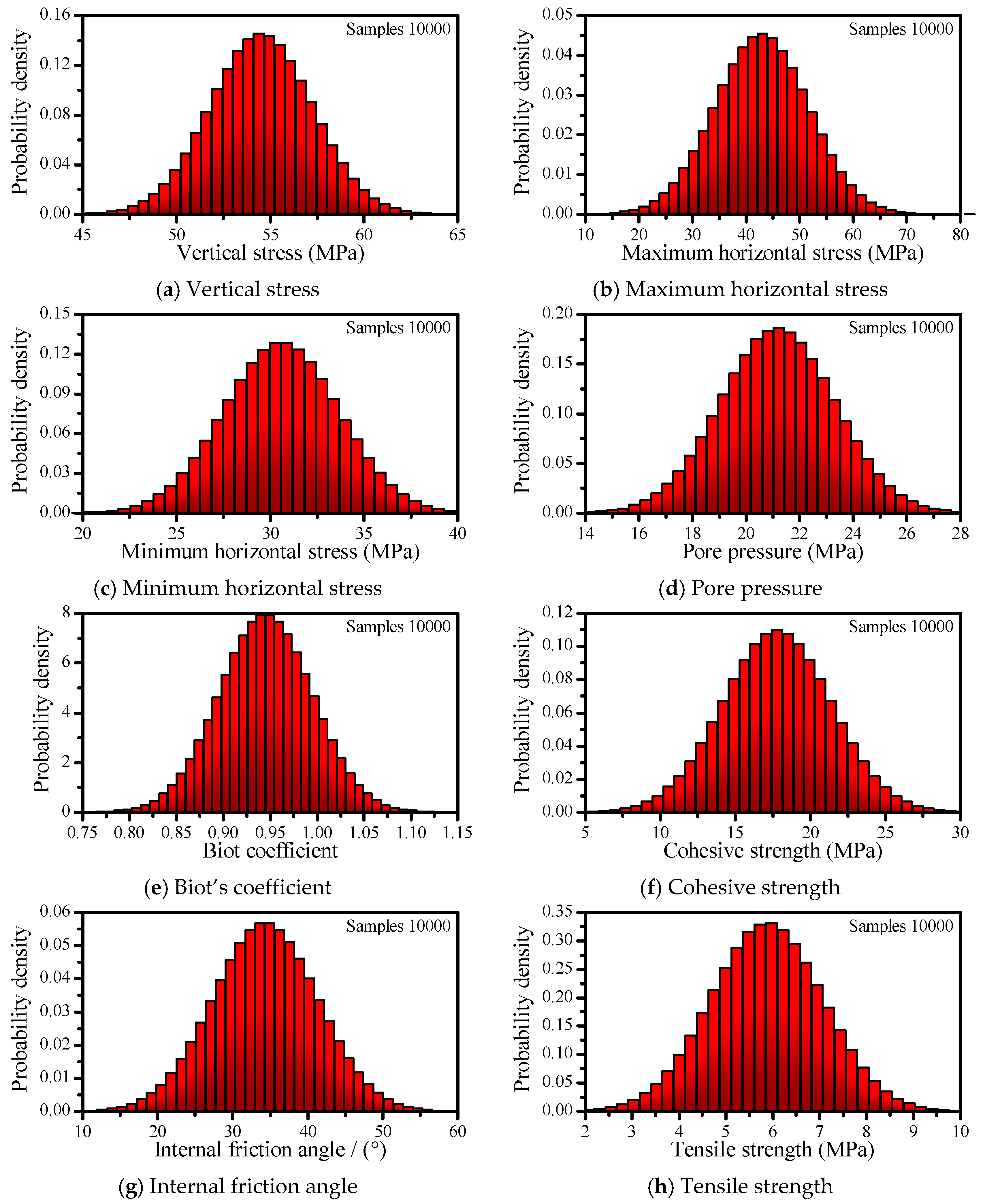
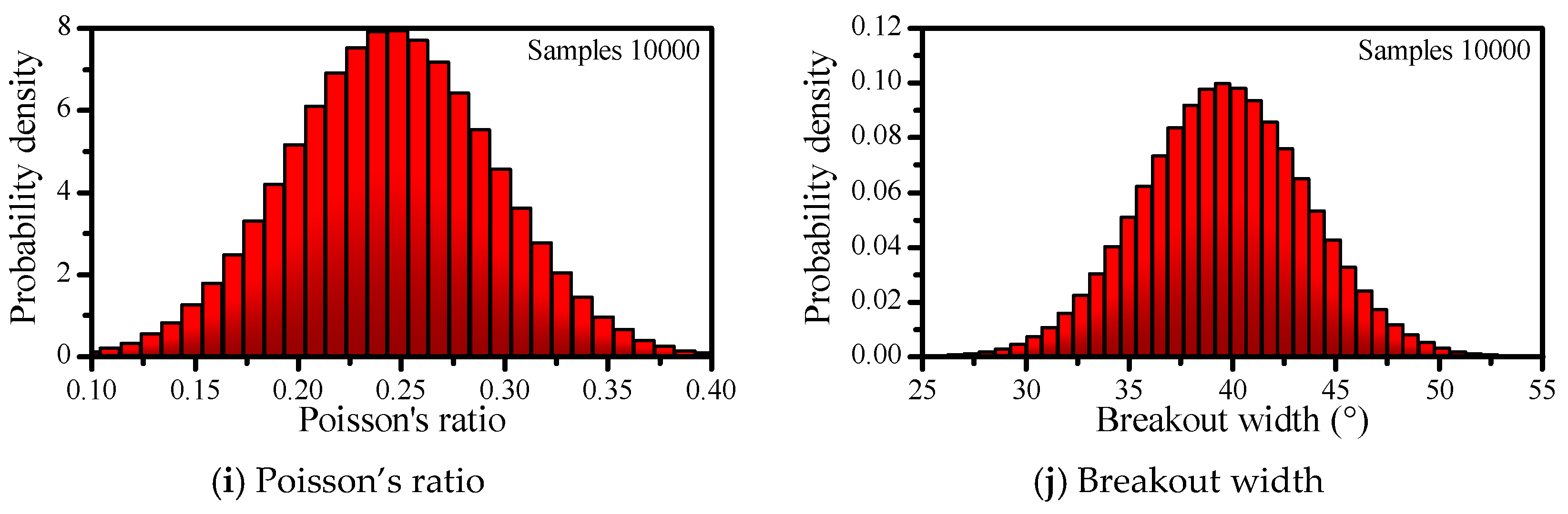
4.1. Uncertainty of Basic Parameters

The basic parameters of wellbore stability analysis are uncertain, and these basic parameters are not exact values but the average estimates [19], and the average values themselves are known to have flaws. The real values are usually variable and following some distribution. As shown in Table 1, the mean value, standard deviation (Std Dev), variance (Var) of each parameter are presented. The mean of the input data were interpreted and identified from logging data. Regarding the choice of random variable distributions, some of the probability distributions normally used in wellbore stability analysis include the uniform distribution, triangular distribution, lognormal distribution, Gamma distribution, Beta distribution, and Weibull distribution [30]. From an engineering perspective, the normal distribution is the preferred choice for wellbore stability problems, due to the distribution functions are mostly normally distributed [38,39]. It should be noticed that the random variable distributions used in this work are based on assumption, but the choice of random variable distributions should be revisited. Regarding the uncertainties in the input data, according to the engineering experience of Aadnøy [21], measurement and interpretation errors are the major sources of input parameter uncertainties [21,23]. Currently, the uncertainties are only “educated guesses” with possibility for future improvements, and the assumed uncertainties in both measurement and interpretation results were listed in

Table 2. Assumed uncertainties in both measurement and interpretation results.

No.	Parameter	Uncertainty in Measurement	Uncertainty in Interpretation
1	Vertical stress	5%	5–10%
2	Maximum horizontal stress	/	10–20%
3	Minimum horizontal stress	5%	5–10%
4	Pore pressure	2–5%	5–30%
5	Biot’s coefficient	/	5–10%
6	Cohesive strength	/	10–50%
7	Internal friction angle	/	10–30%
8	Tensile strength	/	10–50%
9	Poisson’s ratio	/	20–50%

. Although the uncertainties in the input data were based on assumption, the orders of magnitudes of the input data were assumed correct. On this basis, Monte Carlo simulation was utilized with 10,000 iterations. The simulating results of the probability density histogram for basic parameters were shown in Figure 6. It is clearly shown that the uncertain distribution of each parameter satisfies the normal distribution, the higher the coefficient of variance is, the higher the level of uncertainty will be, and the wider the distribution of parameter values will be. The 90% confidence interval (from 5 to 95%, i.e., P5–P95) of each parameter was also listed in Table 1. For example, the 90% confidence interval is 36.64–51.07 MPa for the estimation of maximum horizontal stress, while it’s just 50.29–59.30 MPa, 28.35–33.44 MPa, 17.86–24.90 MPa for the estimations of vertical stress, minimum horizontal stress and pore pressure, respectively. It is clearly shown that the estimation of maximum horizontal stress has a higher confidence interval of P5 and P95, due to its high level of uncertainty.

4.2. Uncertainty Analysis of EMWCP

4.2.1. EMWCP Probability Analysis for both M-C and MG-C Criteria

EMWCP means the equivalent mud weight of collapse pressure, and there are two types of collapse model, i.e., the M-C model and MG-C model. We compared the simulating results between M-C model and MG-C model, the results are shown in Figure 7, the statistics both for M-C model and MG-C model was collected in

Table 3. The statistics of EMWCP both for M-C and MG-C model.

Statistics	EMWCP
	M-C	MG-C
P5/(g/cm3)	0.3221	0.2317
P95/(g/cm3)	0.9825	0.9063
Mean/(g/cm3)	0.6438	0.5538
Analytical solution/(g/cm3)	0.6354	0.5195
Std Dev/(g/cm3)	0.2029	0.2011

. It is clearly found that the same uncertainty in basic parameters results in different answers for M-C model and MG-C model. The analytical solution of the M-C criterion (0.6354 g/cm³) is obviously higher than that of the MG-C criterion (0.5195 g/cm³), and the M-C criterion tends to calculate a higher mean EMWCP (0.6438 g/cm³) than that of the MG-C criterion (0.5538 g/cm³). This depends on the conservative nature of the M-C criterion, due to the M-C criterion ignored the influence of the intermediate principal stress, which makes the required EMW to prevent wellbore collapse is too conservative. However, the MG-C criterion overcame the defect of the M-C criterion. In other words, the M-C criterion under-predicts rock strength and estimates the EMWCP too conservative, while the MG-C criterion rightly predicts rock strength and estimates the EMWCP much more exactly.

As shown in Figure 8, due to the influence of intermediate principal stress for the MG-C criterion, the rock strength increase firstly and then decrease, but the rock strength is much higher than that of the M-C criterion. Moreover, the standard deviation in the M-C criterion is slightly higher than that of the MG-C criterion, which also reveals that the level of uncertainty estimated by MG-C criterion is lesser than that of the M-C criterion. Furthermore, the EMWCP with probability (P95) denotes the minimum possible EMW with probability of 95%, which defines the likelihood of preventing wellbore collapse as a function of EMW, it can be obtained from the cumulative probability curves. The P95 EMWCP estimated by the M-C criterion is 0.9825 g/cm³, while the P95 EMWCP estimated by the MG-C criterion is 0.9063 g/cm³. The minimum possible EMW estimated by the reliability assessment method is obviously higher than that of the analytical solution. In the following section, we just use the MG-C model to analyze the EMWCP.

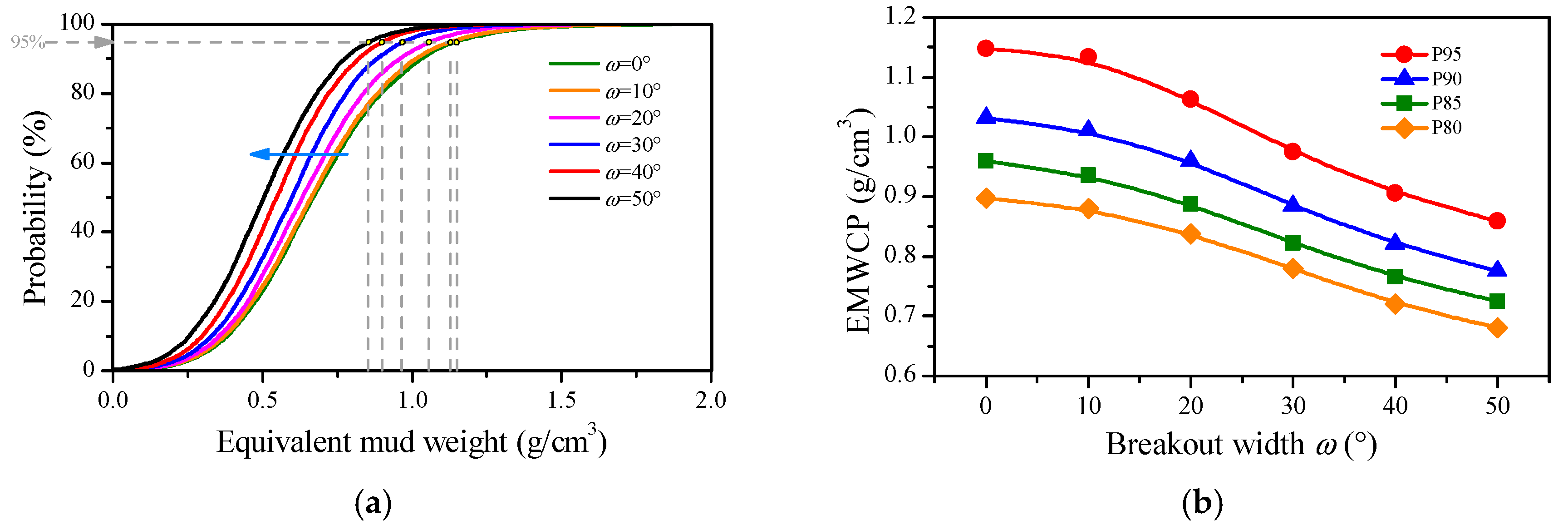
4.2.2. Influence of Breakout Width

As mentioned in the Introduction, the required EMWCP predicted by traditional model is too conservative. The traditional models assume that the critical failure appears at the highest point of stress concentration, in other words, it’s performed to yield no shear failure along the borehole wall. However, the real drilling engineering allows a tolerable breakout or an appropriate breakout width, which do not cause an unbearable collapse problem. The breakout width model was involved to overcome this problem, but it is seldom investigated by traditional models. The influence of mean breakout width was simulated, and the results were shown in Figure 9. For different breakout situation of ω = 0°, ω = 10°, ω = 20°, ω = 30°, ω = 40° and ω = 50°, the P95 EMWCP estimated by the MG-C criterion is 1.1471 g/cm³, 1.1341 g/cm³, 1.0629 g/cm³, 0.9755 g/cm³, 0.9062 g/cm³ and 0.8593 g/cm³ respectively. The relationship between the EMWCP and breakout width were fitted and expressed as follows:

$$\begin{array}{l}{\mathrm{EMWCP}}_{\mathrm{P}95}=4.6858\times {10}^{-6}{\omega }^3-3.8040\times {10}^{-4}{\omega }^2+1.6000\times {10}^{-3}\omega +1.1483\begin{array}{cc}& (R^2=0.9982)\end{array}\\ {\mathrm{EMWCP}}_{\mathrm{P}90}=3.1797\times {10}^{-6}{\omega }^3-2.6884\times {10}^{-4}{\omega }^2+3.8431\times {10}^{-4}\omega +1.0313\begin{array}{cc}& (R^2=0.9990)\end{array}\\ {\mathrm{EMWCP}}_{\mathrm{P}85}=2.5424\times {10}^{-6}{\omega }^3-2.1160\times {10}^{-4}{\omega }^2-4.6500\times {10}^{-4}\omega +0.9596\begin{array}{cc}& (R^2=0.9998)\end{array}\\ {\mathrm{EMWCP}}_{\mathrm{P}80}=2.5092\times {10}^{-6}{\omega }^3-2.2044\times {10}^{-4}{\omega }^2+4.3316\times {10}^{-4}\omega +0.8966\begin{array}{cc}& (R^2=0.9997)\end{array}\end{array}$$

(38)

where EMWCP_P95 is the minimum possible EMWCP with probability of 95%, g/cm³; EMWCP_P90 is the minimum possible EMWCP with probability of 90%, g/cm³; EMWCP_P85 is the minimum possible EMWCP with probability of 85%, g/cm³; EMWCP_P80 is the minimum possible EMWCP with probability of 80%, g/cm³.

It is clearly shown that the EMWCP_P95, EMWCP_P90, EMWCP_P85 and EMWCP_P80 estimated by the MG-C criterion always decline with breakout width in nonlinear. In other words, the EMWCP declines with breakout width, but not the higher the breakout width the better wellbore stability. A more accurate definition of collapse is that when the breakout width or angle exceeds a critical limit, such that the remaining unaffected section of the wellbore wall can no longer uphold the surrounding high stresses and flows inward causing bore enlargement, subsequent collapse and complete failure of the wellbore [21]. Zoback [6] indicated that the tolerable breakout width (2ω) to prevent borehole collapse is approximately 90° for a vertical borehole. Once the breakout width (2ω) exceeds the allowable breakout width, the borehole will cannot maintain itself stability.

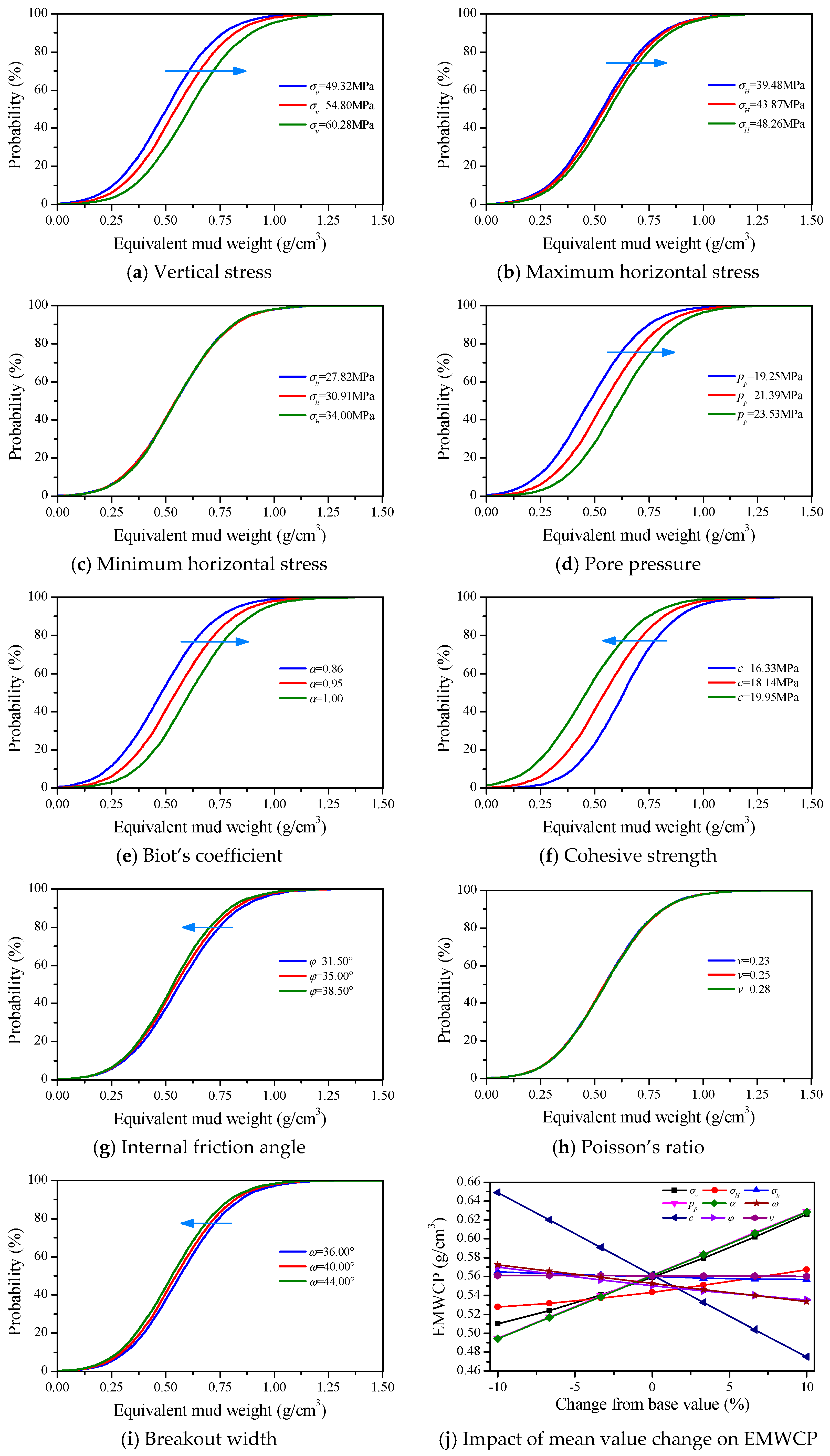
4.2.3. Influence of Mean Value

According to Equations (16), (18) and (22), the EMWCP usually depends on the vertical stress (σ_v), the maximum horizontal stress (σ_H), the minimum horizontal stress (σ_h), the pore pressure (p_p), the Biot’s coefficient (α), the strength parameters (c, φ), the Poisson’s ratio (v), and the tolerable breakout width (ω). The influence of the mean value of each basic parameter is a key aspect to EMWCP. We simulated the influence of different mean value of each basic parameter on the cumulative probability of EMWCP, and the results were shown in Figure 10, where the mean value of each basic parameter was changed ±10% from base value. It is clearly found that the vertical stress, pore pressure, Biot’s coefficient, and cohesive strength had a very strong impact on the cumulative probability of EMWCP, while the other parameters had a lesser impact.

As shown in Figure 10j, it showed the impact of mean value change on EMWCP, all of those basic parameters were changed ±10% from base value, but the corresponding variation of EMWCP gave different answers. The ranking of the influencing degree of mean value change is the cohesive strength > pore pressure ≈ Biot’s coefficient > vertical stress > maximum horizontal stress > breakout width > internal friction angle > minimum horizontal stress > Poisson’s ratio. In general, the EMWCP is positively correlated with the vertical stress, maximum horizontal stress, pore pressure and Biot’s coefficient; while it is negatively correlated with the minimum horizontal stress, cohesive strength, internal friction angle, Poisson’s ratio and breakout width.

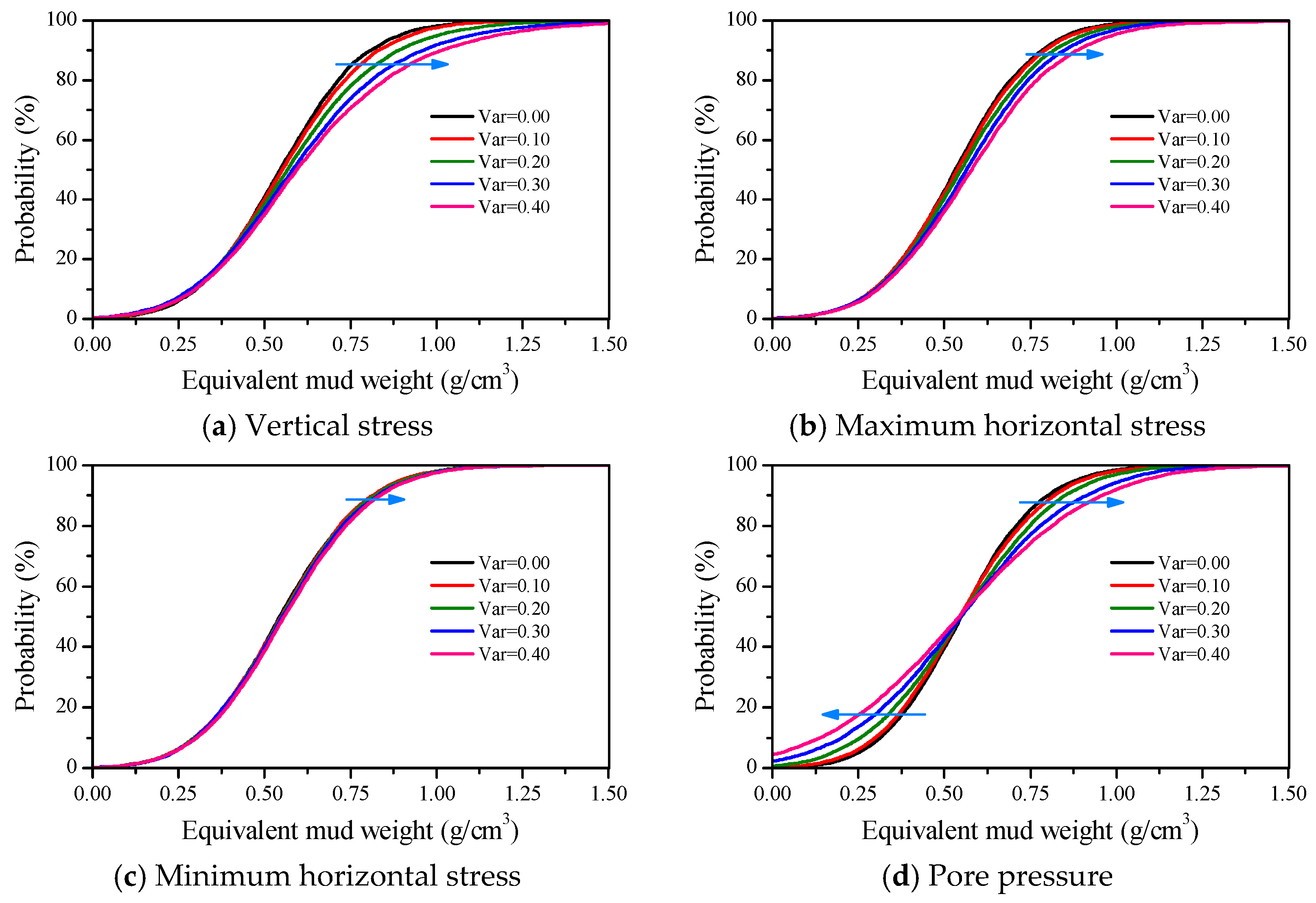
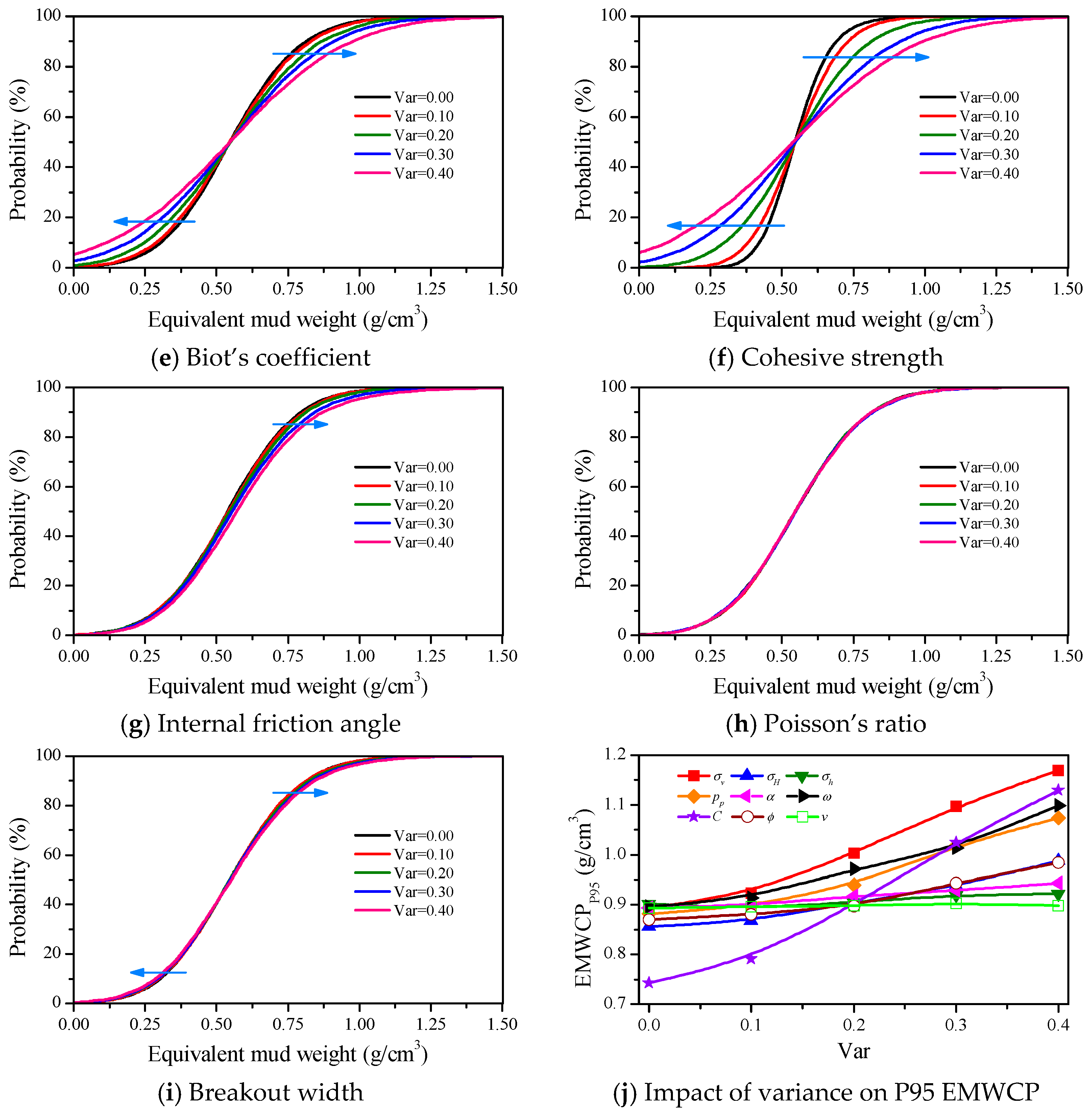
4.2.4. Influence of Variance

Due to the uncertainty of basic parameters, not only the mean value of input parameter affect the EMWCP, but also the uncertainties also affect the EMWCP. In general, the variance represented the degree of uncertainty for a single input parameter. The influences of variance on the cumulative probability of EMWCP were simulated, and the results were shown in Figure 11, where the variance of input parameter was changed from 0.0 to 0.4. It is clearly found that the vertical stress, maximum horizontal stress, pore pressure, Biot’s coefficient, cohesive strength had a very strong impact on the cumulative probability of EMWCP, while the other parameters had a lesser impact. When the variance changes from 0.0 to 0.4, all of the cumulative probability of EMWCP changed, but the corresponding variation of cumulative probability gave different answers. For the vertical stress, maximum horizontal stress, minimum horizontal stress, internal friction angle and Poisson’s ratio, with the increase of variance, the cumulative probability curves gradually moved onto right. But for the pore pressure, Biot’s coefficient, cohesive strength and breakout width, with the increase of variance, the 50–100% of the cumulative probability curves gradually moved onto right, while the 0–50% of the cumulative probability curves gradually moved onto left. In fact, we usually focus on the 50–100% of the cumulative probability curve, thus, with the increase of variance, the cumulative probability curves gradually moved onto right. In other words, the risk of wellbore collapse increases with increase of variance. On the whole, the ranking of the influencing degree of variance is the cohesive strength > Biot’s coefficient > pore pressure > vertical stress > maximum horizontal stress > breakout width > internal friction angle > minimum horizontal stress > Poisson’s ratio. Moreover, we usually focus on the high cumulative probability of the curves, and we just extracted the P95 EMWCP to reveal their influences, the results were shown in Figure 11j. It is clearly found that the P95 EMWCP increase with the variance, and the ranking of the rate of change is the cohesive strength > vertical stress > Biot’s coefficient > pore pressure > maximum horizontal stress > internal friction angle > breakout width > minimum horizontal stress > Poisson’s ratio.

Moreover, a sensitivity analysis was carried out for the EMWCP, the results were shown in Figure 12. The results showed clearly that the influence ranking of the basic parameters is the cohesive strength > Biot’s coefficient > pore pressure > vertical stress > maximum horizontal stress > breakout width > internal friction angle > minimum horizontal stress > Poisson’s ratio. It is consistent with the results of Figure 11. From the risk analysis point of view, we should be concerned with the top five factors which impact the EMWCP the most; and these factors are the cohesive strength, Biot’s coefficient, pore pressure, vertical stress and maximum horizontal stress.

4.3. Uncertainty Analysis of EMWFP

4.3.1. EMWFP Probability Analysis

EMWFP means the equivalent mud weight of fracture pressure, the simulating results is shown in Figure 13. The mean EMWFP estimated by the reliability assessment method is 1.6021 g/cm³, and the analytical solution (1.6020 g/cm³) is very close to the mean EMWFP estimated by the reliability assessment method. The probability decreases with increase of EMW, that means the higher the EMW, the higher the risk of wellbore fracture is. We should determine a proper probability to obtain the corresponding EMWFP, such as the EMWFP with probability (P95) denotes the maximum possible EMW with probability of 95%, which defines the likelihood of preventing wellbore fracture as a function of EMW, it can be obtained from the cumulative probability curves. As shown in Figure 13, the EMWFP estimated by the reliability assessment method is 0.6120 g/cm³, 0.8386 g/cm³, 0.9800 g/cm³ and 1.0834 g/cm³ for the probability of 95%, 90%, 85% and 80% respectively. The maximum possible EMW estimated by the reliability assessment method is obviously lower than that of the analytical solution (1.6020 g/cm³). In other words, the uncertainty of basic parameters results in a lower EMWFP, and the risk of wellbore fracture become much higher.

4.3.2. Influence of Mean Value

According to Equations (30)–(33), the EMWFP is usually depended on the maximum horizontal stress (σ_H), the minimum horizontal stress (σ_h), the pore pressure (p_p), the Biot’s coefficient (α), and the tensile strength (S_t). The influence of the mean value of each basic parameter is a key aspect to EMWFP. We simulated the influence of different mean value of each basic parameter on the cumulative probability of EMWFP, and the results were shown in Figure 14, where the mean value of each basic parameter was changed ±10% from base value. It is clearly found that the maximum horizontal stress, minimum horizontal stress, pore pressure and Biot’s coefficient had a very strong impact on the cumulative probability of EMWFP, while the other parameters had a lesser impact.

As shown in Figure 14f, it showed the impact of mean value change on EMWFP, all of those basic parameters were changed ±10% from base value, but the corresponding variation of EMWFP gave different answers. The ranking of the influencing degree of mean value change is the minimum horizontal stress > the maximum horizontal stress > the Biot’s coefficient ≈ the pore pressure > the tensile strength. The EMWFP is positively correlated with the minimum horizontal stress and the tensile strength, while it is negatively correlated with the maximum horizontal stress, the Biot’s coefficient and the pore pressure.

4.3.3. Influence of Variance

Similarly, not only the mean value of each basic parameter affects the EMWFP, but also the uncertainty can also affect the EMWFP. In general, the variance represented the degree of uncertainty for basic parameter. We simulated the influence of variance on the cumulative probability of EMWFP, and the results were shown in Figure 15, where the variance of each basic parameter was changed from 0.0 to 0.4. It is clearly found that the maximum horizontal stress and the minimum horizontal stress had a very strong impact on the cumulative probability of EMWFP, while the other parameters had a lesser impact. When the variance changed from 0.0 to 0.4, all of the cumulative probability of EMWFP changed. With the increase of variance, the 50–100% of the cumulative probability curves gradually moved onto left, while the 0–50% of the cumulative probability curves gradually moved onto right. In fact, we usually focus on the 50–100% of the cumulative probability curve, thus, with the increase of variance, the cumulative probability curves gradually moved onto left. In other words, the risk of wellbore fracture increases with increase of variance. On the whole, the ranking of the influencing degree of variance is the minimum horizontal stress > the maximum horizontal stress > the Biot’s coefficient > the pore pressure > the tensile strength. Moreover, we usually focus on the high cumulative probability of the curves, and we just extracted the P95 EMWFP to reveal their influences, the results were shown in Figure 15f. It is clearly found that the P95 EMWFP decrease with the variance, and the ranking of the rate of change is also minimum horizontal stress > the maximum horizontal stress > the Biot’s coefficient > the pore pressure > the tensile strength.

Moreover, a sensitivity analysis was carried out for the EMWFP, the results were shown in Figure 16. The results showed clearly that the ranking of the basic parameters is the minimum horizontal stress > the maximum horizontal stress > the Biot’s coefficient ≈ the pore pressure > the tensile strength. It is consistent with the results of Figure 15. From the risk analysis point of view, we should be concerned with the top two factors which impact the EMWFP the most; and these factors are the minimum horizontal stress and the maximum horizontal stress.

4.4. Uncertainty Analysis of EMWPP

EMWPP means the equivalent mud weight of pore pressure, the simulating results is shown in Figure 17. The mean EMWPP estimated by the reliability assessment method is 0.9921 g/cm³, and the analytical solution (0.9921 g/cm³) is also the same. The probability increases with increase of EMW, that means the higher the EMW, the lower the risk of well kick is. We should determine a proper probability to obtain the corresponding EMWPP, such as the EMWPP with probability (P95) denotes the minimum possible EMW with probability of 95%, which defines the likelihood of preventing well kick as a function of EMW, it can be obtained from the cumulative probability curves. As shown in Figure 17, the EMWPP estimated by the reliability assessment method is 1.1552 g/cm³, 1.1192 g/cm³, 1.0949 g/cm³ and 1.0756 g/cm³ for the probability of 95%, 90%, 85% and 80% respectively. The minimum possible EMW estimated by the reliability assessment method is obviously higher than that of the analytical solution (0.9921 g/cm³). In other words, the uncertainty of pore pressure results in a lower EMWPP, and the risk of well kick become much higher.

According to Equations (34)–(36), the EMWPP only depends on the pore pressure (p_p). The influence of the mean value and variance of pore pressure is the key aspect to EMWPP. We simulated the influence of different mean value of pore pressure on the cumulative probability of EMWFP, and the results were shown in Figure 18, where the mean value of pore pressure was changed ±10% from base value. It is clearly found that the uncertain pore pressure had a very strong impact on the cumulative probability of EMWPP. The EMWPP is positively correlated with the mean value of pore pressure. Moreover, we also simulated the influence of variance on the cumulative probability of EMWPP, and the results were shown in Figure 19, where the variance of pore pressure was changed from 0.0 to 0.4. When the variance changed from 0.0 to 0.4, the 50–100% of the cumulative probability curves gradually moved onto right, while the 0–50% of the cumulative probability curves gradually moved onto left. In fact, we usually focus on the 50–100% of the cumulative probability curve, thus, with the increase of variance, the cumulative probability curves gradually moved onto right. In other words, the risk of well kick linearly increased with increase of variance, as shown in Figure 19b.

4.5. Uncertainty Analysis of SMWW

On the basis of the uncertainty analysis of EMWCP, EMWFP and EMWPP, the cumulative probability of SMWW can be obtained, and the results were shown in Figure 20 and Figure 21 and

Table 4. The statistics for EMWPP, EMWCP, EMWFP and SMWW.

Statistics	EMWPP	EMWCP	EMWFP	SMWW
P80/(g/cm3)	1.0756	0.8083	1.0935	1.0756–1.0935
P85/(g/cm3)	1.0949	0.8487	0.9791	No SMWW
P90/(g/cm3)	1.1193	0.9053	0.8240	No SMWW
P95/(g/cm3)	1.1552	0.9063	0.6144	No SMWW
P100/(g/cm3)	1.3734	1.5160	−0.8036	No SMWW
Mean/(g/cm3)	0.9921	0.5538	1.6021	0.9921–1.6021
Std Dev/(g/cm3)	0.0992	0.2060	0.6013	/
Analytical solution/(g/cm3)	0.9921	0.5195	1.6020	0.9921–1.6020

. Figure 20 shows the interference of the probability density function of EMWCP, EMWFP and EMWPP, the overlapping zone denotes the probability of wellbore instability. The smaller overlapping zone, the wellbore will be more reliable, i.e., the risk of wellbore instability will be lower. The bigger overlapping zone, the wellbore will be more unreliable, i.e., the risk of wellbore instability will be higher.

Figure 21 shows the cumulative probability of EMWCP, EMWFP and EMWPP, and the statistics all for EMWCP, EMWFP and EMWPP were collected in Table 4. It is clearly found that when the uncertainty of basic parameters is considered, the mean EMWCP is 0.5538 g/cm³, and the P95 EMWCP is 0.9063 g/cm³, while the analytical solution (0.5195 g/cm³) is obviously too low to maintain wellbore stability, that is, the collapse risk of the wellbore is actually much higher than that of traditional analysis. Similarly, when the uncertainty of basic parameters is considered, the mean EMWPP is 0.9921 g/cm³, and the P95 EMWPP is 1.1552 g/cm³, while the analytical solution (0.9921 g/cm³) is obviously lower, that is, the kick risk of the well is actually much higher than that of traditional analysis. Moreover, when the uncertainty of basic parameters is considered, the mean EMWFP is 1.6021 g/cm³, and the P95 EMWFP is 0.6144 g/cm³, while the analytical solution (1.6020 g/cm³) is obviously lower, that is, the fracture risk of the wellbore is actually much higher than that of traditional analysis.

According to the Equation (37), the lowest safe mud weight of SMWW should be depended on the high of EMWCP and EMWPP, and the highest safe mud weight of SMWW should be depended on the EMWFP, that is, the lowest safe mud weight should be the EMWPP, while the highest safe mud weight should be the EWMCP. As shown in Figure 21 and Table 4, when the cumulative probability is 95%, the P95 EMWFP (0.6144 g/cm³) is obviously lower than both of EMWPP (1.1552 g/cm³) and EMWCP (0.9063 g/cm³), there is no SMWW. When the cumulative probability is 90%, the P90 EMWFP (0.8240 g/cm³) is obviously lower than both of EMWPP (1.1193 g/cm³) and EMWCP (0.9053 g/cm³), there is still no SMWW. When the cumulative probability is 85%, the P85 EMWFP (0.9791 g/cm³) is obviously lower than EMWPP (1.0949 g/cm³) but higher than EMWCP (0.8487 g/cm³), that is, there is still no SMWW. When the cumulative probability is 80%, the P80 EMWFP (1.0935 g/cm³) is obviously higher than both of EMWPP (1.0756 g/cm³) and EMWCP (0.8083 g/cm³), there is a SMWW of 1.0756–1.0935 g/cm³, but it is very narrow SMWW. The SMWW predicted by analytical solution is 0.9921–1.6020 g/cm³, compared to the SMWW estimated by the reliability assessment method, the SMWW predicted only by mean value is very wide to maintain wellbore stability, but the reliability assessment method tends to give a narrow SMWW of 1.0756–1.0935 g/cm³ and its probability is only 80%, that is, it is very difficult to drill without any wellbore instability problems. In this situation, the traditional over-balanced drilling (OBD) maybe cannot drill successfully, but there is an available mud weight window (0.8083–1.0935 g/cm³) to avoid wellbore collapse and fracture, we maybe can utilize underbalanced drilling (UBD), managed pressure drilling (MPD), or micro-flow drilling (MFD) to conquer well kick, and we can drill successfully. Another choice should be wider the SMWW, the only way is to prevent lost circulation.

4.6. Field Observation Report

In the design of well SC-101X, the traditional OBD was designed to drill in the 2008–2432 m section, the density of water-based drilling mud was designed as 1.07 g/cm³ by considering the impact of the surge and swab pressures. In real drilling operation, the actual drilling mud density was also 1.07 g/cm³. When this well was drilled at the depth of 2022 m, the driller operates drilling rig to pull the drill string up and down to prepare making a connection, the mud man found drilling mud loss, the average loss rate of drilling mud was approximately 3.67 m³/h, and the total loss volume of drilling mud was approximately 10.5 m³. In this process, the drilling mud was added some lost circulation materials (LCMs) to against drilling mud loss, the LCMs formula was given as follows: 4% GZD-B + 5% GZD-C + 6% GZD-D. After multiple plugging, the pressure-bearing capacity was tested, and the lost pressure was enhanced to 1.19 g/cm³. The drilling mud density of 1.07 g/cm³ was still used to drill. But when this well was drilled at the depth of 2067 m, the driller operates drilling rig to pull the drill string up and down to prepare making a connection, the mud man found a gas kick. The well was shut-in to prepare well kill. After testing the shut-in standpipe pressure, the killing mud density was determined as 1.13 g/cm³. During well killing, the drilling mud loss occurred again with a low average loss rate of 3.5 m³/h. After the well was killed successfully, and considering the higher pore pressure of the lower formation, the use of MPD was considered. Before drilling using MPD, the drilling mud was again added some lost circulation materials (LCMs), and the LCMs formula was given as follows: 5% GZD-O + 5% GZD-A + 10% GZD-B + 10% GZD-C + 14% GZD-D + 4% FDJ-1 + 3% Nutshell + 3% JD-5. After multiple plugging, the pressure-bearing capacity was tested, and the lost pressure was enhanced to 1.37 g/cm³. In the process of MPD, the operating parameters were listed in

Table 5. Operating parameters of MPD.

No.	Parameters	Value
1	Well depth (m)	2067–2432
2	EMWPP (g/cm3)	1.08
3	EMWCP (g/cm3)	1.09 (Enhanced to 1.37)
4	Mud displacement (L/s)	20–25
5	Mud density (g/cm3)	1.05–1.16
6	Pressure control during drilling (MPa)	0–1
7	Pressure control during pump-stopping (MPa)	2–3

, and finally, the section of 2067–2432 m of well SC-101X was drilled successfully. To sum up, the field observation for well kick and wellbore fracture is consistent with analysis results of SMWW that estimated by uncertain model. Thus, the present model was therefore verified, and it is much more accurate than the traditional analytical solution.

5. Conclusions

On the basis of the reliability assessment theory, the uncertain EMWCP model was proposed by involving the tolerable breakout and the MG-C criterion, the uncertain EMWFP and EMWPP model was also proposed, and the uncertain SMWW model was determined by EMWCP, EMWPP and EMWFP. Finally, taking the basic parameters of well SC-101X as an example, the influence of uncertain basic parameter on SMWW was systematically investigated and discussed. The main conclusions can be drawn as follows:

(1)

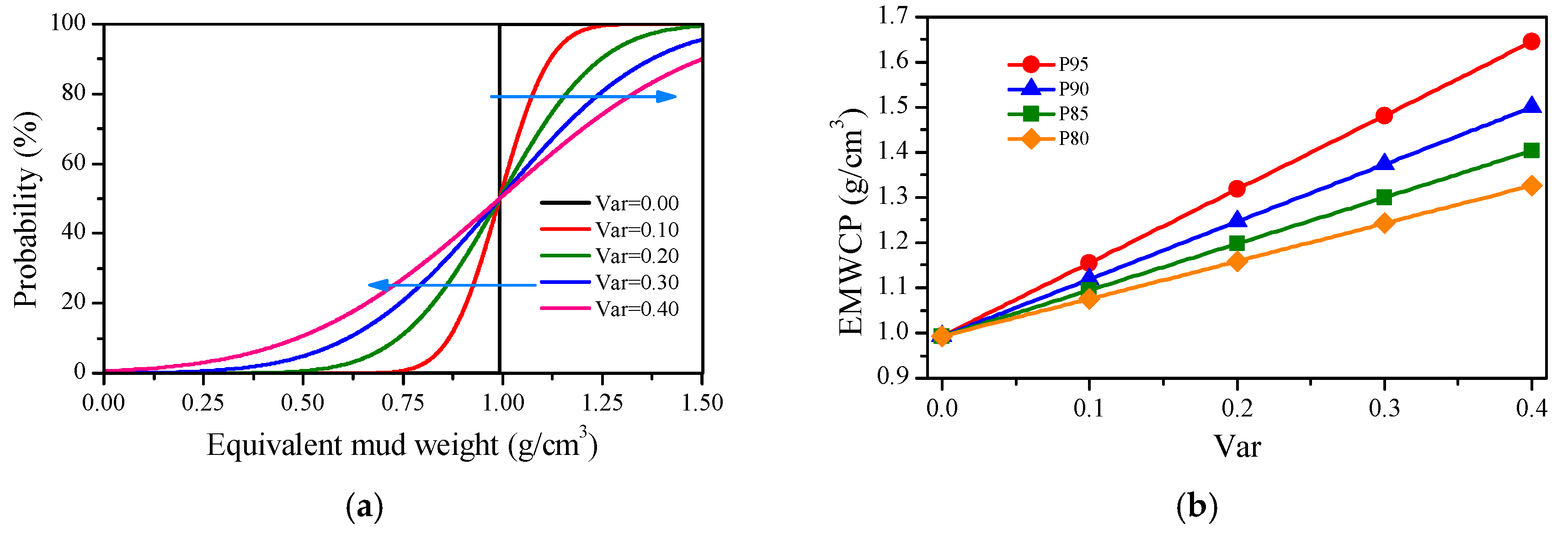
For wellbore stability analysis, the uncertain distribution of each basic parameter satisfies the normal distribution, the higher the coefficient of variance is, the higher the level of uncertainty will be, and the larger the impact on wellbore stability will be.

(2)

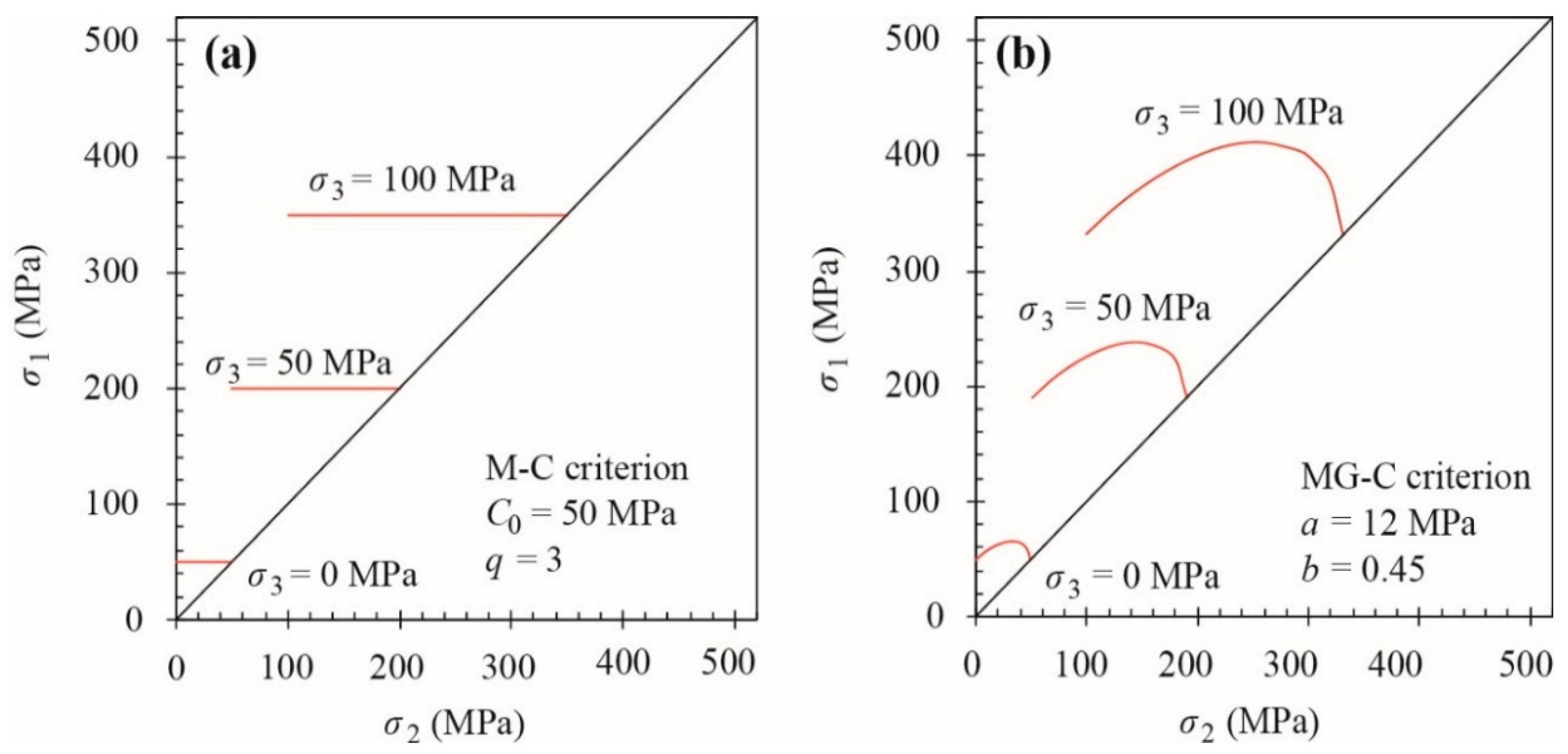
The EMWCP predicted by the M-C criterion is obviously higher than that of the MG-C criterion, because of the MG-C criterion rightly predicts rock strength and estimates the EMWCP much more exactly. Thus, the MG-C criterion is recommended for wellbore stability analysis.

(3)

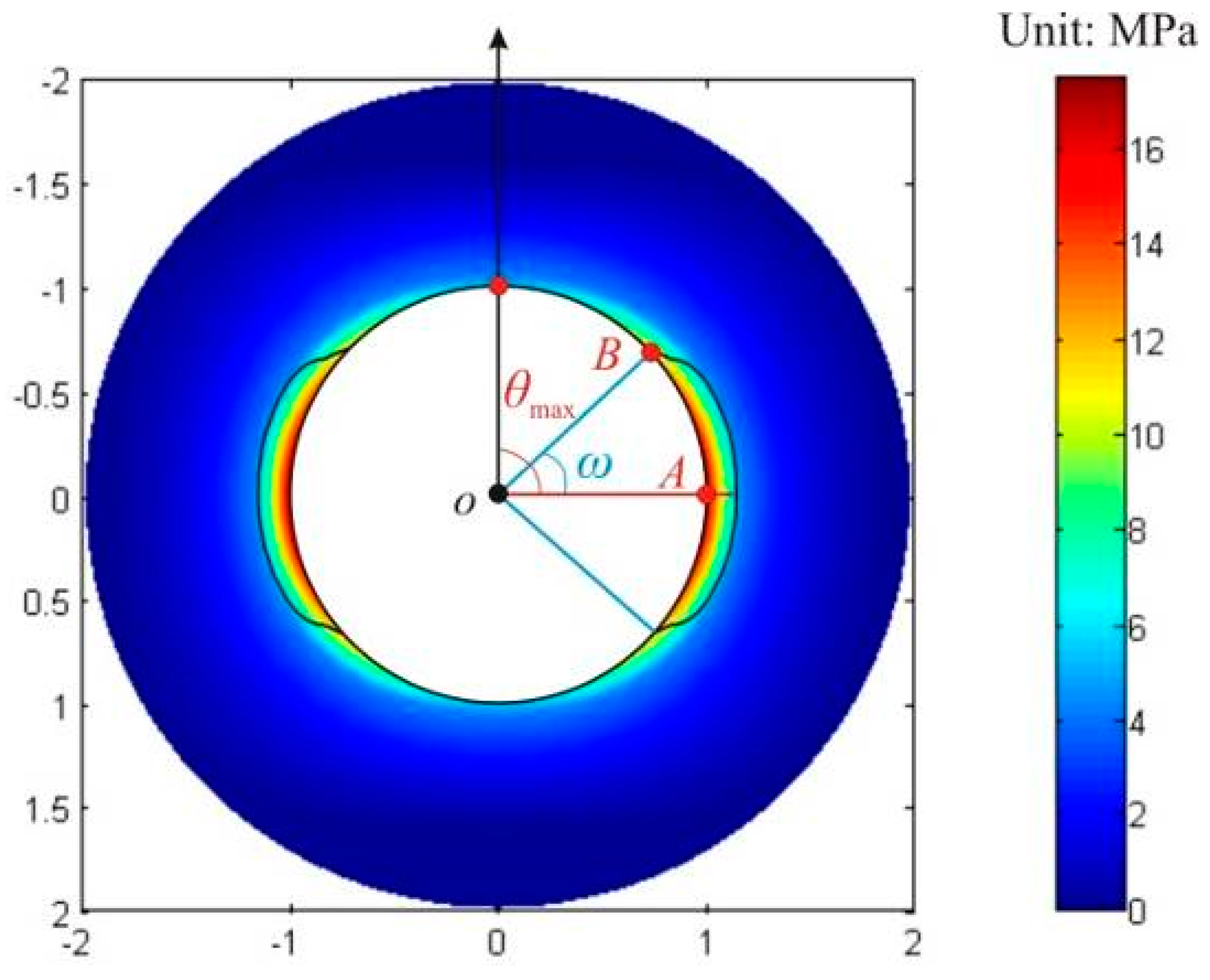
The breakout width has a very significant impact on EMWCP, and the EMWCP always decline with breakout width in nonlinear. The tolerable breakout is recommended for wellbore stability analysis, and the tolerable breakout width (2ω) of 45° is recommended for a vertical well.

(4)

The EMWCP estimated by the uncertain model is obviously higher than that of analytical model, that is, the collapse risk of the wellbore is heightened by the uncertain basic parameters. The cumulative probability of wellbore collapse gradually increases with increasing of variance, and the influencing degree of uncertain basic parameter is the cohesive strength > Biot’s coefficient > pore pressure > vertical stress > maximum horizontal stress > breakout width > internal friction angle > minimum horizontal stress > Poisson’s ratio.

(5)

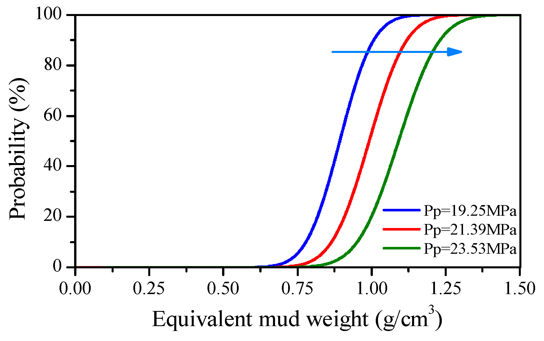
The EMWPP estimated by the uncertain model is obviously higher than that of mean pore pressure, that is, the kick risk is also heightened by the uncertain pore pressure. The cumulative probability of well kick gradually also increases with increasing of variance for pore pressure.

(6)

The EMWFP estimated by the uncertain model is obviously lower than that of analytical model, that is, the fracture risk of the wellbore heightened by the uncertain basic parameters. The cumulative probability of wellbore fracture gradually increases with increasing of variance, and the influencing degree of uncertain basic parameter is the minimum horizontal stress > maximum horizontal stress > Biot’s coefficient > pore pressure > tensile strength.

(7)

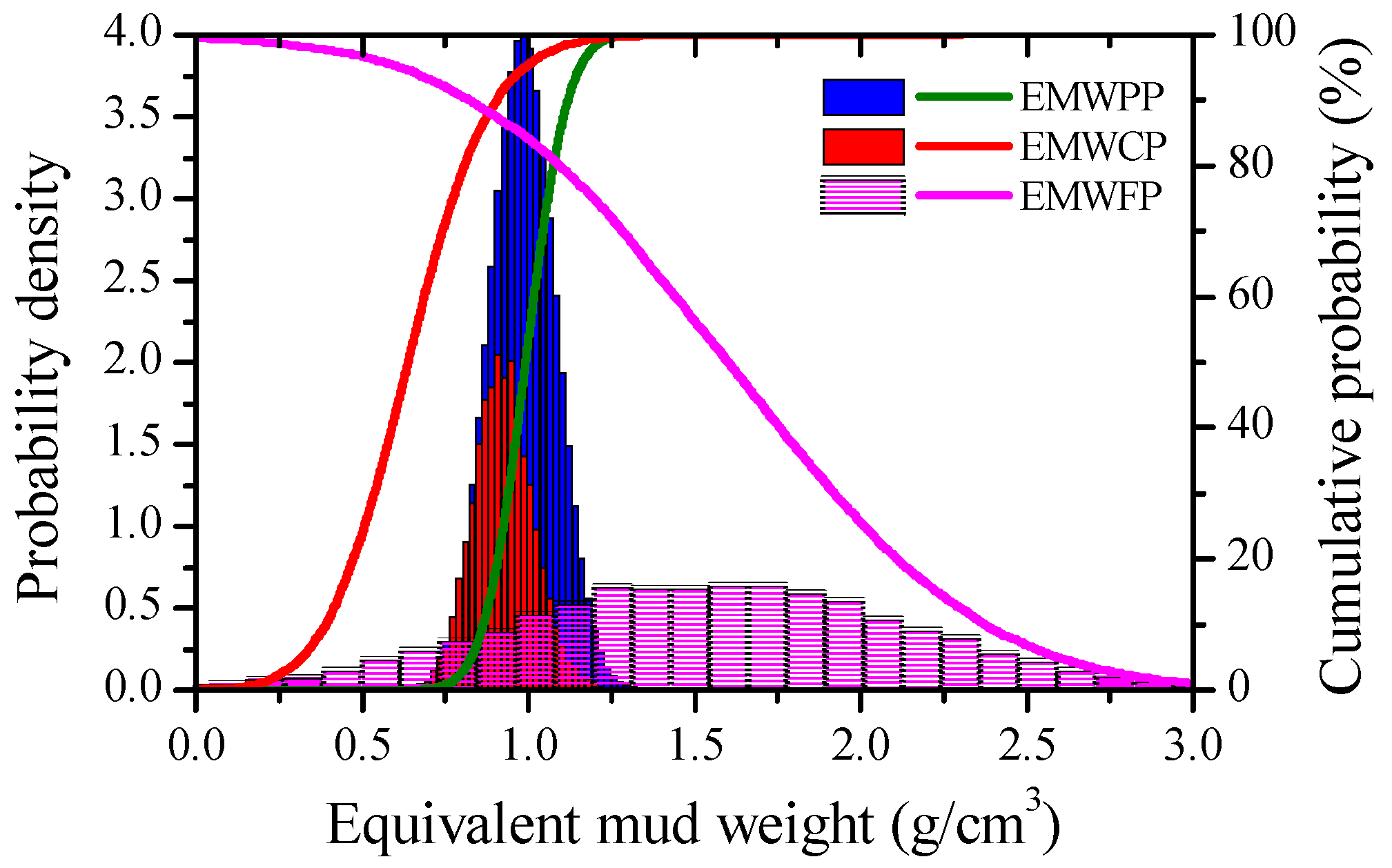
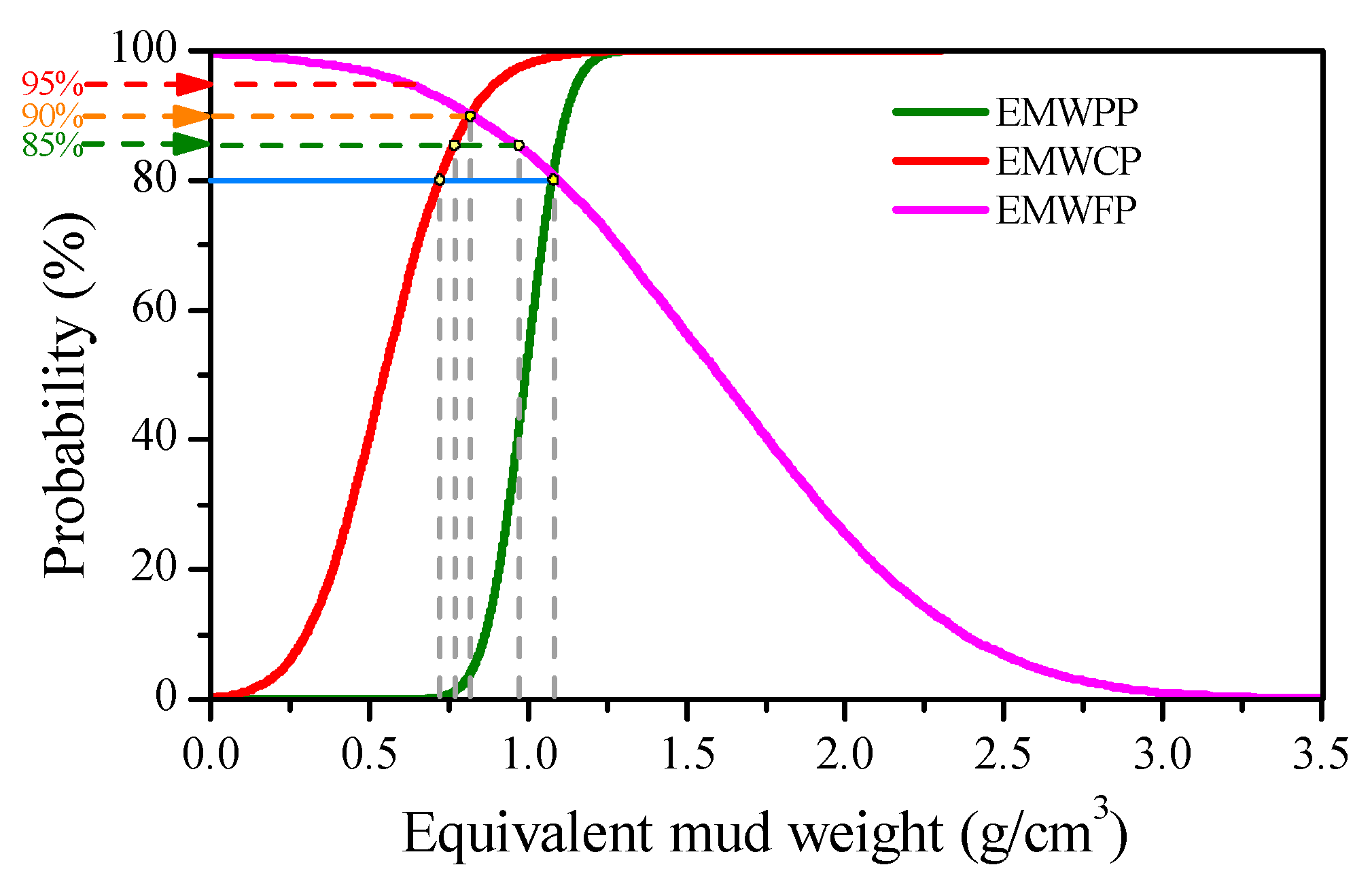
For the SC-101X well, the SMWW predicted by analytical solution is 0.9921–1.6020 g/cm³ and very wide, compared to the SMWW estimated by the uncertain model, the P80 SMWW estimated by the uncertain model is only 1.0756–1.0935 g/cm³ and very narrow, that is, there is a low possibility to drill without any wellbore instability problems. The field observation for well kick and wellbore fracture verified the analysis results of SMWW that estimated by uncertain model, and both lost circulation prevention and MPD were utilized to maintain drilling safety.

(8)

To drill the formation with narrow SMWW, some kinds of advanced drilling technology, such as the UBD, MPD and MFD, can be utilized to control the wellbore pressure accurately, so that the wellbore stability can be maintained. Meanwhile, another choice should be wider the SMWW, the only way is to prevent lost circulation.

References

1. Ma, T.; Chen, P.; Zhao, J. Overview on vertical and directional drilling technologies for the exploration and exploitation of deep petroleum resources. Geomech. Geophys. Geo-Energy Geo-Resour. 2016, 2, 365–395. [Google Scholar] [CrossRef] [Green Version]
2. Ma, T.S.; Chen, P.; Yang, C.H.; Zhao, J. Wellbore stability analysis and well path optimization based on the breakout width model and Mogi-Coulomb criterion. J. Pet. Sci. Eng. 2015, 135, 678–701. [Google Scholar] [CrossRef]
3. Fjar, E.; Holt, R.M.; Raaen, A.M.; Risnes, R. Petroleum Related Rock Mechanics, 2nd ed.; Elsevier: Amsterdam, The Netherlands, 2008; pp. 309–339. [Google Scholar]
4. Aadnoy, B.; Looyeh, R. Petroleum Rock Mechanics: Drilling Operations and Well Design; Gulf Professional Publishing: Oxford, UK, 2011; pp. 65–296. [Google Scholar]
5. Chen, M.; Jin, Y.; Zhang, G. Rock Mechanics of Petroleum Engineering; Science Press: Beijing, China, 2008; pp. 55–130. [Google Scholar]
6. Zoback, M.D. Reservoir Geomechanics; Cambridge University Press: Oxford, UK, 2007; pp. 167–339. [Google Scholar]
7. Al-Ajmi, A.M.; Zimmerman, R.W. Stability analysis of vertical boreholes using the Mogi-Coulomb failure criterion. Int. J. Rock Mech. Min. Sci. 2006, 43, 1200–1211. [Google Scholar] [CrossRef]
8. Al-Ajmi, A.M.; Zimmerman, R.W. A new well path optimization model for increased mechanical borehole stability. J. Pet. Sci. Eng. 2009, 69, 53–62. [Google Scholar] [CrossRef]
9. Ma, T.S.; Chen, P. A wellbore stability analysis model with chemical-mechanical coupling for shale gas reservoirs. J. Nat. Gas Sci. Eng. 2015, 26, 72–98. [Google Scholar] [CrossRef]
10. Ma, T.S.; Chen, P.; Zhang, Q.B.; Zhao, J. A novel collapse pressure model with mechanical-chemical coupling in shale gas formations with multi-weakness planes. J. Nat. Gas Sci. Eng. 2016, 36, 1151–1177. [Google Scholar] [CrossRef]
11. Ma, T.S.; Zhang, Q.B.; Chen, P.; Yang, C.H.; Zhao, J. Fracture pressure model for inclined wells in layered formations with anisotropic rock strengths. J. Pet. Sci. Eng. 2017, 149, 393–408. [Google Scholar] [CrossRef]
12. Ma, T.S.; Yang, Z.X.; Chen, P. Wellbore stability analysis of fractured formations based on Hoek-Brown failure criterion. Int. J. Oil Gas Coal Technol. 2018, 17, 143–171. [Google Scholar] [CrossRef]
13. Ma, T.S.; Liu, Y.; Chen, P.; Wu, B.S.; Fu, J.H.; Guo, Z.X. Fracture-initiation pressure prediction for transversely isotropic formations. J. Pet. Sci. Eng. 2019, 176, 821–835. [Google Scholar] [CrossRef]
14. Morita, N. Uncertainty analysis of borehole stability problems. In Proceedings of the SPE Annual Technical Conference & Exhibition, Dallas, TX, USA, 22–25 October 1995. [Google Scholar]
15. McLellan, P.J.; Hawkes, C.D. Application of probabilistic techniques for assessing sand production and borehole instability risks. In Proceedings of the SPE/ISRM Rock Mechanics in Petroleum Engineering, Trondheim, Norway, 8–10 July 1998. [Google Scholar]
16. Ottesen, S.; Zheng, R.H.; McCann, R.C. Wellbore stability assessment using quantitative risk analysis. In Proceedings of the SPE/IADC Drilling Conference, Amsterdam, The Netherlands, 9–11 March 1999. [Google Scholar]
17. De Fontoura, S.A.B.; Holzberg, B.B.; Teixeira, E.C.; Frydman, M. Probabilistic analysis of wellbore stability during drilling. In Proceedings of the SPE/ISRM Rock Mechanics Conference, Irving, TX, USA, 20–23 October 2002. [Google Scholar]
18. Moos, D.; Peska, P.; Finkbeiner, T.; Zoback, M. Comprehensive wellbore stability analysis utilizing quantitative risk assessment. J. Pet. Sci. Eng. 2003, 38, 97–109. [Google Scholar] [CrossRef]
19. Sheng, Y.; Reddish, D.; Lu, Z. Assessment of uncertainties in wellbore stability analysis. In Modern Trends in Geomechanics; Wu, W., Yu, H.S., Eds.; Springer: Berlin, Germany, 2006; pp. 541–557. [Google Scholar]
20. Al-Ajmi, A.M.; Al-Harthy, M.H. Probabilistic wellbore collapse analysis. J. Pet. Sci. Eng. 2010, 74, 171–177. [Google Scholar] [CrossRef]
21. Aadnøy, B.S. Quality assurance of wellbore stability analyses. In Proceedings of the SPE/IADC Drilling Conference and Exhibition, Amsterdam, The Netherlands, 1–3 March 2011. [Google Scholar]
22. Zhong, L.; Yan, X.; Tian, Z.; Yang, H.; Yang, X. A collapse pressure analysis in reservoir drilling based on the reliability method. Acta Pet. Sin. 2012, 33, 477–482. [Google Scholar]
23. Udegbunam, J.E.; Aadnøy, B.S.; Fjelde, K.K. Uncertainty evaluation of wellbore stability model predictions. J. Pet. Sci. Eng. 2014, 124, 254–263. [Google Scholar] [CrossRef]
24. Kinik, K.; Wojtanowicz, A.K.; Gumus, F. Temperature-induced uncertainty of the effective fracture pressures: Assessment and control. In Proceedings of the SPE Deepwater Drilling and Completions Conference, Galveston, TX, USA, 10–11 September 2014. [Google Scholar]
25. Kinik, K.; Wojtanowicz, A.K.; Gumus, F. Probabilistic assessment of the temperature-induced effective fracture pressures. Spe Drill. Complet. 2016, 31, 40–52. [Google Scholar] [CrossRef]
26. Gholami, R.; Rabiei, M.; Rasouli, V.; Aadnoy, B.; Fakhari, N. Application of quantitative risk assessment in wellbore stability analysis. J. Pet. Sci. Eng. 2015, 135, 185–200. [Google Scholar] [CrossRef]
27. Plazas, F.; Calderon, Z.; Quintero, Y. Wellbore stability analysis: A stochastic approach applied to a colombian cretaceous formation. In Proceedings of the SPE Latin American and Caribbean Petroleum Engineering Conference, Quito, Ecuador, 18–20 November 2015. [Google Scholar]
28. Kanfar, M.F.; Chen, Z.; Rahman, S.S. Risk-controlled wellbore stability analysis in anisotropic formations. J. Pet. Sci. Eng. 2015, 134, 214–222. [Google Scholar] [CrossRef]
29. Phoon, K.K.; Ching, J. Risk and Reliability in Geotechnical Engineering; CRC Press: Boca Raton, FL, USA, 2014; pp. 131–179. [Google Scholar]
30. Baecher, G.B.; Christian, J.T. Reliability and Statistics in Geotechnical Engineering; John Wiley & Sons: Chichester, UK, 2003; pp. 303–432. [Google Scholar]
31. Liao, H.; Guan, Z.; Yan, Z.; Ma, G. Assessment method of casing failure risk based on structure reliability theory. Acta Pet. Sin. 2010, 31, 161–164. [Google Scholar]
32. Li, Q.; Tang, Z. Optimization of wellbore trajectory using the initial collapse volume. J. Nat. Gas Sci. Eng. 2016, 29, 80–89. [Google Scholar] [CrossRef]
33. Zhao, K.; Han, J.; Dou, L.; Feng, Y. Moderate collapse in a shale cap of a nearly depleted reservoir. Energies 2017, 10, 1820. [Google Scholar] [CrossRef]
34. Zhang, H.; Yin, S.; Aadony, B.S. Poroelastic modeling of borehole breakouts for in-situ stress determination by finite element method. J. Pet. Sci. Eng. 2018, 162, 674–684. [Google Scholar] [CrossRef]
35. Ma, T.S.; Peng, N.; Tang, T.; Wang, Y.H. Wellbore stability analysis by using a risk-controlled method. In Proceedings of the 52nd US Rock Mechanics/Geomechanics Symposium, Seattle, WA, USA, 17–20 June 2018. [Google Scholar]
36. Li, X.; Jaffal, H.; Feng, Y.C.; Mohtar, C.E.; Gray, K.E. Wellbore breakouts: Mohr-Coulomb plastic rock deformation, fluid seepage, and time-dependent mudcake buildup. J. Nat. Gas Sci. Eng. 2018, 52, 515–528. [Google Scholar] [CrossRef]
37. Li, X.; El Mohtar, C.S.; Gray, K.E. Modeling progressive breakouts in deviated wellbores. J. Pet. Sci. Eng. 2019, 175, 905–918. [Google Scholar] [CrossRef]
38. Mondal, S.; Chatterjee, R. Quantitative risk assessment for optimum mud weight window design: A case study. J. Pet. Sci. Eng. 2019, 176, 800–810. [Google Scholar] [CrossRef]
39. Udegbunam, J.E.; Arild, Ø.; Fjelde, K.K.; Ford, E.; Lohne, H.P. Uncertainty based approach for predicting the operating window in UBO Design. SPE Drill. Complet. 2013, 28, 326–337. [Google Scholar] [CrossRef]
40. Zhang, L.; Cao, P.; Radha, K.C. Evaluation of rock strength criteria for wellbore stability analysis. Int. J. Rock Mech. Min. Sci. 2010, 47, 1304–1316. [Google Scholar] [CrossRef]
Figure 1. Typical wellbore instability. (a) Stable borehole; (b) Enlarged borehole; (c) Borehole breakout; (d) Restricted borehole; (e) Borehole fracture.
Energies 12 00942 g001
Figure 2. Probability densities for the resistances (RC) and loads (QC) of wellbore collapse.
Energies 12 00942 g002
Figure 3. The stress distribution on the borehole wall.
Energies 12 00942 g003
Figure 4. The required cohesion to keep wellbore stability (Modified from [2]).
Energies 12 00942 g004
Figure 5. Schematic representation of breakout growth (Reproduced from [6]). (a) The theoretical model after the formation of wellbore breakouts, wellbore breakouts deepen but do not widen; (b) The measured breakout widths compared very well with those predicted by the simple theory.
Energies 12 00942 g005
Figure 6. Probability density histogram of basic parameters.
Energies 12 00942 g006aEnergies 12 00942 g006b
Figure 7. Probability histogram of EMWCP both for M-C and MG-C model.
Energies 12 00942 g007
Figure 8. Plot of strength criteria in {σ1-σ2} space (Modified from [40]). (a) M-C criterion; (b) MG-C criterion.
Energies 12 00942 g008
Figure 9. Influence of breakout on EMWCP. (a) The cumulative probability of EMWCP; (b) EMWCP varies with breakout width.
Energies 12 00942 g009
Figure 10. Influence of mean value on cumulative probability of EMWCP.
Energies 12 00942 g010
Figure 11. Influence of variance on probability of EMWCP.
Energies 12 00942 g011aEnergies 12 00942 g011b
Figure 12. Sensitivity tornado for EMWCP.
Energies 12 00942 g012
Figure 13. Probability density and cumulative probability for EMWFP.
Energies 12 00942 g013
Figure 14. Influence of mean value on cumulative probability of EMWFP.
Energies 12 00942 g014
Figure 15. Influence of variance on cumulative probability of EMWFP.
Energies 12 00942 g015
Figure 16. Sensitivity tornado for EMWFP.
Energies 12 00942 g016
Figure 17. Probability density and cumulative probability for EMWPP.
Energies 12 00942 g017
Figure 18. Influence of mean value of pore pressure on cumulative probability for EMWPP.
Energies 12 00942 g018
Figure 19. Influence of pore pressure variance on EMWPP. (a) Influence of variance of pore pressure; (b) EMWCP varies with variance.
Energies 12 00942 g019
Figure 20. Probability density histogram of SMWW.
Energies 12 00942 g020
Figure 21. Cumulative probability of SMWW.
Energies 12 00942 g021