Weighted-PSO Applied to Tune Sliding Mode Plus PI Controller Applied to a Boost Converter in a PV System

Abstract

In this paper, a sliding mode plus proportional-integral (PI) controller for a boost converter in a photovoltaic system is proposed. The proposed controller is characterized by being easy to implement and by operating with constant switching frequency. The parameters of the proposed controller are calculated using the weighted particle swarm optimization technique, ensuring low percentage of overshoot and short setting time. The use of this optimization technique allows one to ensure the stability of the controller. A linear lead-leg controller is considered in order to compare the performance of the proposed controller. Finally, experimental results using a solar kit are presented to verify the performance of the proposed controller.

1. Introduction

Currently, the use of renewable energies is increasing due to the need to reduce the negative effects on the environment produced by the use of fossil fuels, such as the greenhouse effect and climate change. Among the renewable energies, photovoltaic (PV) solar energy stands out for being clean, inexhaustible, easy to obtain, and low maintenance [1]. PV energy has received a lot of attention since it gives the possibility of generating electricity both in isolated conditions and connected to network systems.

A disadvantage of PV systems is related to the low conversion of solar energy into electrical energy. The power generated is strongly influenced by environmental conditions such as solar radiation and the temperature of the PV module. For this reason, to increase the power of the system some methods are used to operate at the maximum power point of the PV module. Several maximum power point tracking (MPPT) algorithms have been presented in the literature [2], from the simplest ones such as the constant voltage method [3] or open-circuit voltage method [4], through to the most used ones such as Perturb and Observe [5] or Incremental Conductance [6], to the most sophisticated ones using artificial intelligence techniques such as Fuzzy Logic [7], Neural Networks [8], or genetic algorithms. However, the performance of the MPPT is strongly linked to the controller used to regulate the given reference variable and its ability to respond to sudden changes [9].

Generally, voltage regulation is performed using some linear controller, such as a proportional-integral (PI) or a lead-leg controller [9,10,11]. The use of this type of controller leads to the response having a high percentage of overshoot, a significant setting time, and a considerable steady-state error. Another drawback in the use of linear controllers is the need to linearize the PV system at a specific point of operation in order to design the controller. Therefore, the use of linear controllers may not be adequate because PV systems are highly dependent under environmental conditions and need to provide good performance in all ranges of PV operation. Recently, intelligent control techniques have been proposed to improve these drawbacks. An intelligent-type controller used for various applications is the Fuzzy Logic controller, characterized by its fast response, accuracy, and robustness [12]. Another intelligent controller used for controlling DC converters is the Artificial Neural Network, which can learn and respond to any disturbance or input rapid variation [13].

A suitable option to control the PV voltage or PV current is to use sliding mode control (SM). This type of control is a kind of non-linear control developed for variable structure systems, which is characterized by being robust and dynamic. It is used in power electronics applications, such as DC-DC converters in PV systems [14]. A type of SM is proposed in [15] to regulate the MPPT voltage. This controller is called Double Integral Sliding Mode MPPT Control (DISMC) and uses the double integral of the voltage error to eliminate the error in stable state. However, the design of this controller requires following an arduous mathematical analysis procedure. On the other hand, in [16] the procedure to project an SM to regulate the input voltage of a single-ended primary-inductor converter (SEPIC) is presented. However, this controller uses hysteresis modulation which produces variable switching frequency. Other works such as [1,17,18] have also used SM to regulate the MPPT voltage, showing robust responses to disturbances in the load and to variations in environmental conditions. Nevertheless, the project of these controllers needs complicated mathematical analysis. The use of this SM plus PI controller has been reported in the literature for motor and generator control applications [19,20]. This controller is characterized by operating with constant switching frequency, eliminating the problem of operating with high switching frequencies. Several methods to project controllers have been proposed in the literature. Traditionally, the PI controller is one of the most studied controllers, being tuned using different techniques. In [21], Fuzzy Logic is used to continuously tune the gains of a PI controller applied to regulate the reactive power of a photovoltaic inverter. In relation to the sliding mode controller, the works in the literature use the method of Lyapunov [22,23,24] to guarantee the stability and project the controller; a process that requires a complex mathematical adjustment.

The optimization methods are based on the premise of finding the best possible result under certain circumstances. In optimization problems, the highest or lowest value that a given function (objective function) can take is sought. The optimization methods seek to find the values of the variables that minimize or maximize the objective function while complying with some restrictions [25]. Hence, one can be a powerful tool for controller design.

Particle Swarm Optimization (PSO) [26] is a technique inspired from bird flocking, fish schooling, or bee interaction in search of food applied to the optimization of non-linear problems. This technique in general works on two basic principles: learning from previous data and current communication with the agent of the swarm [27]. In this algorithm each particle has a position that represents a possible solution of the objective function, these particles move according to their personal experiences $P_{best}$ and to the experiences of the group $G_{best}$ to find the solution that takes the objective function to a minimum value. Additionally, PSO was applied to tune PI gains of a distributed static synchronous compensator [28], inverse optimal controller [29], or MPPT SM [30] as an alternative to the classical design. Although, the PSO algorithm lacks an inner mechanism for dealing with constraints. In this way, a double-modified algorithm (-w) and the Dynamic Objective Constraint Handling Method were proposed in [31] to increase the convergence speed and to overcome the problem of premature convergence of the algorithm. This technique of optimization applied to the project of sliding mode controllers for the regulation of the current and the voltage in a photovoltaic system has not been used in other works, which allows us to provide an alternative for the project of this type of controller.

The proposal of this paper is the SM plus PI (SMPI) controller applied to control the inductor current and voltage input of a boost converter of PV system tuned by w-PSO. The w-PSO technique applied to the adjustment of the parameters of the SMPI controller improves the response by ensuring stability and low oscillations without requiring complex mathematical analysis. The SMPI controller is characterized by operating with constant switching frequency, eliminating the problem of operating with high switching frequencies. The results obtained in a experimental setup endorse the proposal and the superior performance can be verified when compared with a lead-leg controller.

This paper is structured as follows. A system description is presented in Section 2. The proposed sliding mode plus PI controller and its design are shown in Section 3. The method to calculate the parameters of the controller using the Particle Swarm Optimization is described in Section 4. Results using a solar kit are given in Section 5. Finally, conclusions are presented in Section 6.

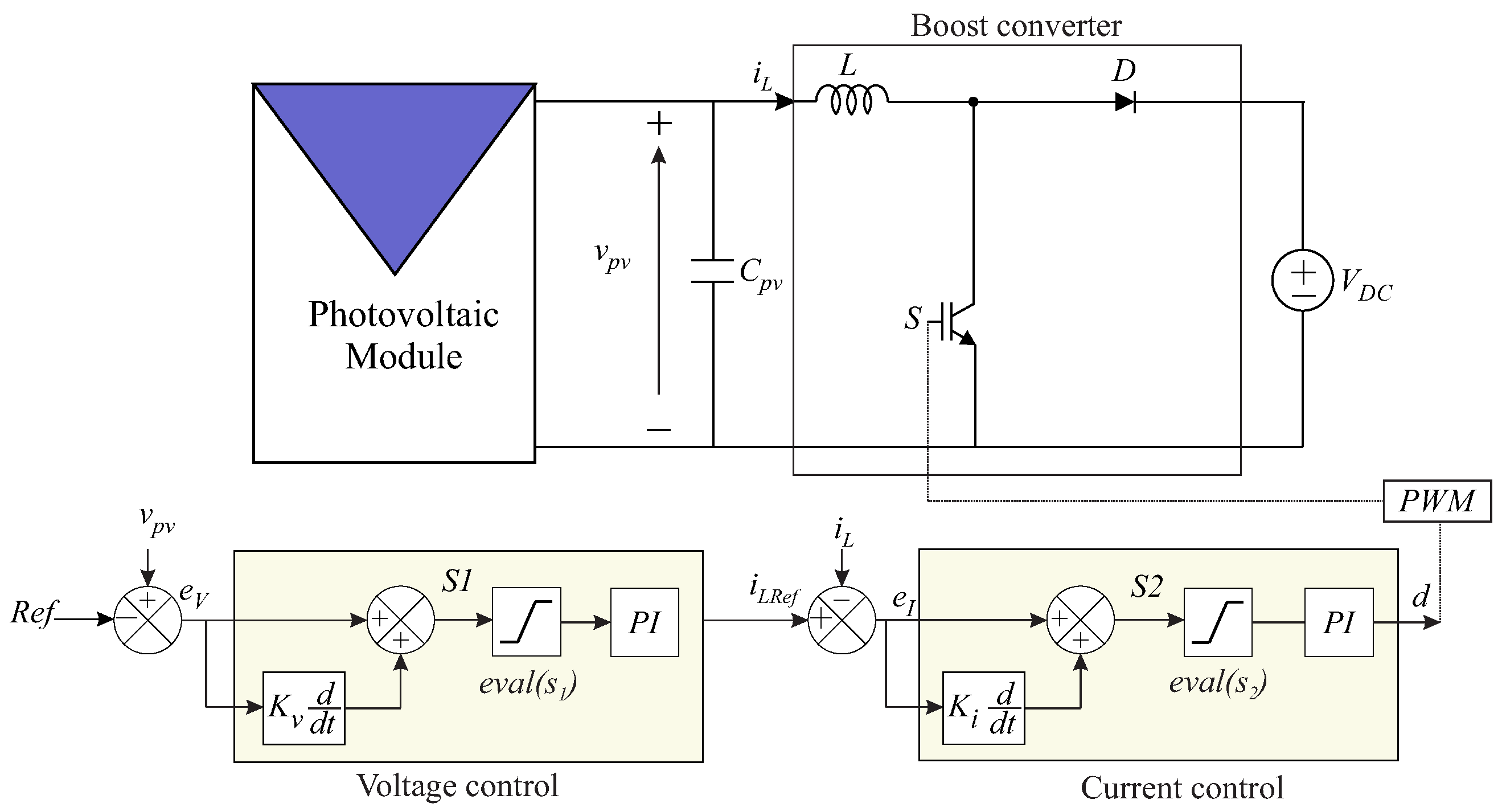
2. System Description

The photovoltaic system considered in this paper is shown in Figure 1. It is composed of a photovoltaic module, a DC-DC boost converter, and a DC source connected to the output as a load. In this paper a boost converter is employed to control the PV panel voltage. The boost converter is composed of an inductor (L), a switch (S), and a diode (D). The control scheme is based on the concept of a double control loop. In this way, the internal loop controls the inductor current ($i_L$) through the change in the duty cycle (d) and the external loop controls the capacitor voltage ($v_{pv}$) through the change in the reference of current. The reference voltage is given by some MPPT method, such as incremental conductance, perturb and observe, or any other. Figure 1 shows the schemes of the proposed controller that will be detailed later. A constant voltage source is used as a load since it simplifies the analysis, giving the possibility of representing systems with a battery charge or systems with a second conversion stage [32].

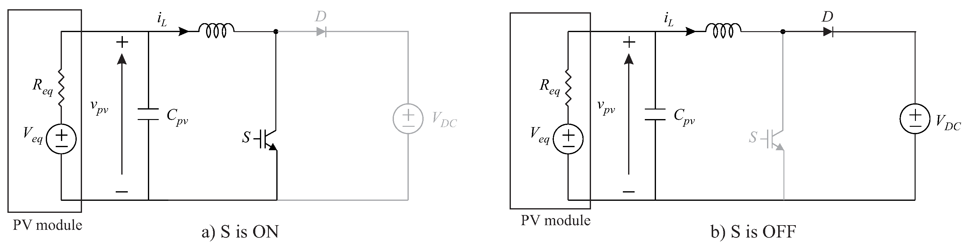
Boost Converter Model

The boost converter is used in photovoltaic systems to implement some algorithm maximum power point tracker (MPPT) through the control of its switch. The boost converter is so called because the output voltage is greater than the input voltage [12], and its topology is shown in Figure 1. The operation of the converter could be described in the following way: When the switch S is turned on by the PWM signal, the current flows through the inductor L storing energy in it. When switch S is turned off, the energy stored in the inductor in the form of an electromagnetic field generates an induced voltage. The induced voltage in the inductor and the input voltage are in series and the sum of them generates the resulting output voltage [33].

In relation to the design of the boost converter, a new approach for sizing the converter parameters specifically for PV applications where the non-linear behavior of the PV module is taken into account is presented in [34].

To obtain a linear equivalent model of the circuit, a method to linearize the photovoltaic module at an operating point is presented in [32]. Generally, the point of operation is selected at the maximum power point since the system is expected to operate at this point. The linear model is described by a straight line tangent to the curve I-V of the PV module at the point of operation. As a result, a constant voltage source ($V_{eq}$) and an equivalent resistance ($R_{eq}$) are obtained. In Figure 2 the two states of operation of the converter including the equivalent PV module are shown.

The dynamic equations corresponding to the state of the circuit when the switch S is ON are obtained by evaluating the derivatives of the inductor current and the capacitor voltage using Figure 2a, as shown in Equations (1) and (2).

$$\frac{d{i}_L\left(t\right)}{dt}=\frac{v_{pv}\left(t\right)}{L}$$

(1)

$$\frac{d{v}_{pv}\left(t\right)}{dt}=\frac{V_{eq}-v_{pv}\left(t\right)}{R_{eq}{C}_{pv}}-\frac{i_L\left(t\right)}{C_{pv}}$$

(2)

When the switch is OFF the dynamic equations are found by evaluating the derivatives of the inductor current and the capacitor voltage using the circuit of Figure 2b. The equations are given in Equations (3) and (4).

$$\frac{d{i}_L\left(t\right)}{dt}=\frac{v_{vp}\left(t\right)-V_{DC}}{L}$$

(3)

$$\frac{d{v}_{pv}\left(t\right)}{dt}=\frac{V_{eq}-v_{pv}\left(t\right)}{R_{eq}{C}_{pv}}-\frac{i_L\left(t\right)}{C_{pv}}$$

(4)

To obtain the small-signal transfer functions, the average variables method can be used. This method allows to eliminate high frequency components maintaining the natural behavior of the system. The modeling process consists of: adding the variables of small signal in the average equations of the circuit, applying the Laplace transform, and manipulating the equations to obtain the desired transfer functions [9]. The detailed procedure for obtaining these functions using a boost converter is shown in [10], from which Equations (5) and (6) are taken, which correspond to the duty cycle-to-inductor current transfer function ($G_{i-d}$) and the inductor current to input voltage transfer function ($G_{v-i}$). The notation of the circumflex accent $\widehat{x}$ in the variables indicates that it is the small signal component.

$$G_{i-d}=\frac{{\widehat{i}}_L}{\widehat{d}}=\frac{V_{DC}(1+s{R}_{eq}{C}_{pv})}{s^2{C}_{pv}L{R}_{eq}+sL+R_{eq}}$$

(5)

$$G_{v-i}=\frac{{\widehat{v}}_{pv}}{{\widehat{i}}_L}=\frac{R_{eq}}{s{C}_{pv}{R}_{eq}}$$

(6)

3. Sliding Mode Plus PI Control

The sliding mode control is a type of non-linear control characterized by being robust against perturbations and variations in the parameters of the system. Sliding mode control is known to belong to a class of variable structure control systems that have been used in power electronics to adequately control systems of variable nature such as DC-DC converters [35]. Its principle of operation consists of moving the trajectory of the states of the system towards a predetermined surface known as sliding surface and ensuring that the states remain in the vicinity of it through a control law [36].

The conventional sliding mode controllers operate at a very high and variable switching frequency, which can cause an increase in switching losses and interference by electromagnetic noise [35]. Thus, in this work a controller sliding mode plus PI (SMPI) is used, characterized by operating with constant switching frequency and being easy to implement.

There are two essential steps in the project of a sliding modes control that are: definition of the sliding surface and design of the control law [37]. These two steps will be explained below.

3.1. Definition of the Sliding Surface

The sliding surface is defined according to the control objectives of the system [37]. Then, the control objectives for the system studied are related to the error between the measured variable and the reference, since the control scheme aims to reduce the error to zero. The sliding surface is defined through the voltage error ($e_v$) and the current error ($e_i$):

$$e_v=v_{pv}-v_{pv,ref}$$

(7)

$$e_i=i_{L,Ref}-i_L$$

(8)

However, to increase the dynamic response of the controller to the errors defined in Equations (7) and (8) its derivatives are added, obtaining the sliding surface set, S, given in Equation (9):

$$S=\left[\begin{array}{c}{s}_1\\ s_2\end{array}\right]=\left[\begin{array}{c}{e}_v+k_v\frac{d{e}_v}{dt}\\ e_i+k_i\frac{d{e}_i}{dt}\end{array}\right]$$

(9)

where the constants $k_v$ and $k_i$ are defined according to the desired dynamics.

3.2. Design of the Control Law

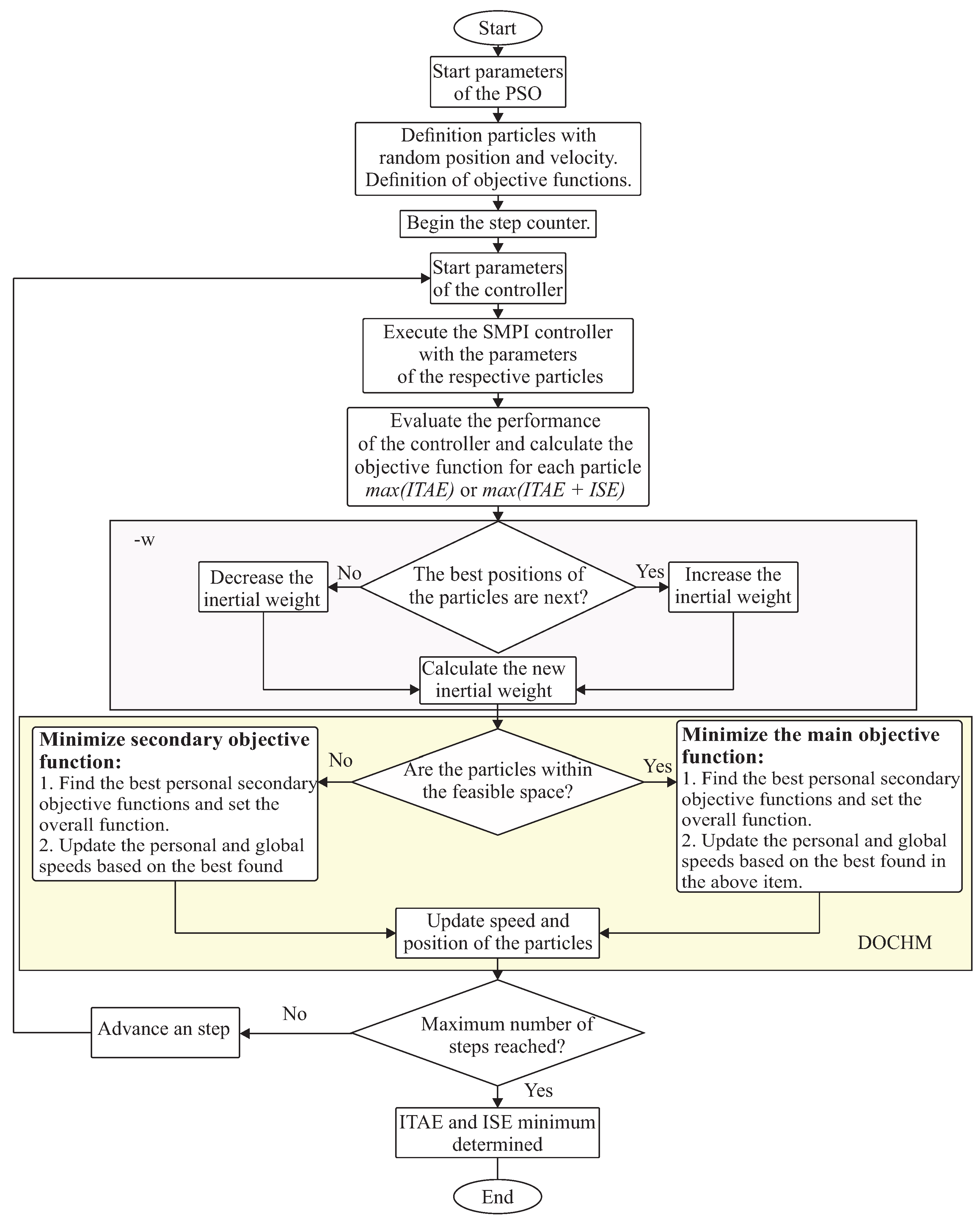
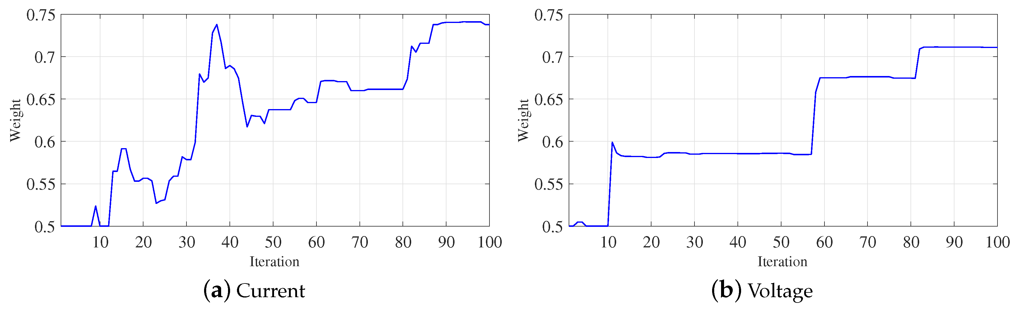
Once the sliding surfaces have been determined, the next step is to define the control law that leads to the trajectories of the system towards the sliding surface and also ensure that they remain on it.

The trajectory S is switched through the $eval\left(s\right)$ function, where this function is also responsible for determining the reaction of the system to changes in the state variables. To implement the $eval$ function a linear function with saturation is used, which operates by limiting the surface when it reaches one of its maximum or minimum values and also, due to its linear nature, it is sensitive to the reduction of the ripple when the state approximates the switching surface [19].

To define the initial phase of the controller, a proportional-integral (PI) controller is used, this initial phase is characterized by the states of the system that have not yet reached the sliding surface [20]. The gains of the PI controller must be appropriately selected in such a way that there is a balance between the transient response and low oscillation. Thus, a high value of the proportional gain will increase the oscillations in the transient state, while a high value of the integral gain could generate an almost linear response. The PI controller added to the sliding modes control reduces the chattering effect, an effect that is present in the sliding mode controllers which is characterized by introducing high frequency vibrations into the system, caused mainly by the high switching frequency [38]. In this way, the controller operates with constant switching frequency.

The control laws for the two control loops correspond to the following two Equations:

$$i_{Lref}=\left(k_{pv}+\frac{k_{iv}}{s}\right)eval\left(s_1\right)$$

(10)

$$d=\left(k_{pc}+\frac{k_{ic}}{s}\right)eval\left(s_2\right)$$

(11)

where $k_{pv}$, $k_{iv}$, $k_{pc}$, and $k_{ic}$ are gains of an integral proportional controller (PI) and $s_1$ and $s_2$ are presented in Equation (9).

Figure 1 shows the schematics of the proposed controller, where sliding surfaces, PI controllers, and $eval$ functions are specified.

The development of the proposed controller requires the tuning of the following parameters: $k_v$ and $k_i$ that correspond to the gains of the error derivative, the upper and lower limits of the two saturators, and the gains of the PI controllers. In total for each control loop it is necessary to tune 5 variables. The selection of this parameters directly affects the controller’s performance. The correct tuning of these variables generates a stable and robust response. In this paper, the particle swarm optimization (PSO) method is used to calculate these parameters. In this way, PSO allows one to obtain the optimal parameters of the controller, improving the transient response and the error in the steady state [39]. Simulation results of the SMPI controller used to regulate the voltage and the input current of a two-level interleaved boost converter were presented in [40]. The parameters of the controller in [40] were tuned through empirical adjustment, while for this article the tuning of the parameters is done through the w-PSO method. This approach allows us to ensure the reliability and performance of the controller, furthermore it presents an innovation since this method has not been previously used to tune SMPI type controllers applied to converters for photovoltaic systems.

4. w-PSO

This algorithm is used to find the optimal values of the SMPI voltage and current controllers. The search process implements the control scheme given in Figure 1. Each control loop is analyzed separately; in this way, it starts with the current loop applying a reference step and calculating the overshoot ($M_p$) and the settling time ($t_{ss}$). Once the optimal values of the current controller have been found, a voltage reference step is applied to analyze again the overshoot and the settling time of the voltage controller.

The optimization process is guided by an objective function, which will be minimized during the execution of the algorithm. The purpose of applying PSO in the search of the parameters of the controllers is to obtain a transient response quickly and without oscillations and an error in minimum stable state. The decision variables of the problem correspond to the parameters of each controller (k, $k_i$, $k_p$, $li{m}_{\mathrm{low}}$, $li{m}_{\mathrm{up}}$). Since there are two controllers, first the algorithm is executed to find the parameters of the current controller, and once calculated the algorithm is executed again to find the parameters of the voltage controller. The objective function is defined by the integral of time multiplied by the absolute value of error (ITAE) [41] and by the integral of the squared error (ISE). ITAE is indicated to reduce the contribution of errors that remain over time, while ISE is indicated to reduce large errors by being insensitive to small errors [42]. For the adjustment of the current controller it is expected that the response has small overshoot and low oscillations, so the ITAE criterion is used to evaluate the response after applying a current reference. In the case of adjustment of the voltage controller in addition to considering the ITAE criterion, the ISE criterion is also considered, since the adjustment of this loop must be stricter because this controller provides the current reference. The ITAE for the current and voltage controllers is calculated using Equations (12) and (13), respectively. The ISE used for the current controller is calculated using (14).

$$\begin{array}{c}\hfill ITA{E}_i={\int }_0^{\tau }t|e_i\left(t\right)|dt={\int }_{t_{step,i}}^{t_{step,i}+t_0}(t-t_{step,i})|i_{L,ref}\left(t\right)-i_L\left(t\right)|dt\end{array}$$

(12)

$$\begin{array}{c}\hfill ITA{E}_v={\int }_0^{\tau }t|e_v\left(t\right)|dt={\int }_{t_{step,v}}^{t_{step,v}+t_0}(t-t_{step,v})|v_{pv}\left(t\right)-v_{pv,ref}\left(t\right)|dt\end{array}$$

(13)

$$ISE={\int }_0^{\tau }{e}_i^2\left(t\right)dt={\int }_{t_{step,i}}^{t_{step,i}+t_0}{(i_{L,ref}\left(t\right)-i_L\left(t\right))}^{2}dt$$

(14)

where $t_{step,i}$ and $t_{step,v}$ are the instants in which the step is applied in the current and voltage references. $e_i$ and $e_v$ are the errors of current and voltage.

The search space of the algorithm is limited by the restrictions of $M_p$ and $t_{ss}$, being considered for both controllers a maximum $M_p$ of 10% and $t_{ss}$ of 15 ms.

In this algorithm, each particle has a position that represents a possible solution of the objective function. These particles move according to personal experience ($P_{best}$), that is, the best position the particle found in previous iterations, according to the global experience ($G_{best}$), which is related to the best positions of the group and according its actual velocity (${\overrightarrow{W}}_{vel}\left(k\right)$). Since they are two controllers, there are two optimization problems, defined in Equations (15) and (16). The problem given in (15) corresponds to the current loop, while (16) to the voltage loop.

$$\begin{array}{cc}\underset{\overrightarrow{W}\in S}{\mathrm{minimize}}& \left\{ITA{E}_i\right\}\\ \mathrm{subject} \mathrm{to}& M_p<10\% \mathrm{and} t_{ss}<15\end{array}$$

(15)

$$\begin{array}{cc}\underset{\overrightarrow{W}\in S}{\mathrm{minimize}}& \{ITA{E}_v,ISE\}\\ \mathrm{subject} \mathrm{to}& M_p<10\% \mathrm{and} t_{ss}<15\end{array}$$

(16)

where S is the search space and $\overrightarrow{W}$ is the vector that includes the parameters of the SMPI controller.

The update of the position of a particle (j) is realized through the sum of the velocity vector with the current position:

$$W_i^j(k+1)=W_i^j+{\overrightarrow{W}}_{vel,i}^j(k+1)$$

(17)

While the particle velocity update is a linear combination of the current velocity, the best personal experience, and the best global experience:

$$\begin{array}{c}{W}_{vel,i}^j(k+1)=\underset{\mathrm{Actual} \mathrm{velocity}}{\underbrace{w_{PSO}·W_{vel,i}}}+\underset{\mathrm{Best} \mathrm{personal} \mathrm{experience}}{\underbrace{c_p·\mathrm{rand}\left(\right[1,0\left]\right)(W_{best,P,i}^j\left(k\right)-W_i^j\left(k\right))}}+\hfill \\ \underset{\mathrm{Best} \mathrm{global} \mathrm{experience}}{\underbrace{c_g·\mathrm{rand}\left(\right[1,0\left]\right)(W_{best,G,i}^j\left(k\right)-W_i^j\left(k\right))}}\hfill \end{array}$$

(18)

where rand([1, 0]) represents a random value between 0 and 1. $c_p$ and $c_g$ are the acceleration factors that multiply the vectors with the best personal position and the best global position, respectively. Finally, $w_{PSO}$ is the inertial weight of the particle that determines if the particle continues moving in the same direction.

The PSO used in this work is a double-modified algorithm (-w) and Dynamic Objective Constraint Handling Method (DOCHM). The first variation (w-PSO) consists of dynamically modifying the inertial weight of the particles [31]. This inertial weight is constantly updated through a feedback of the best particle positions. This change allows to alternate between the exploration and research processes. Thus, when the inertial weight increases it means that the particles are close, allowing one to better investigate the search region. In addition, when the inertial weight decreases, the algorithm is exploring a new search region, avoiding convergence in a local optimum.This modified PSO requires that the acceleration coefficients $c_p$ and $c_g$ have a constant value of 1.5 and that the following relationship between the sum of them and the inertial weight of the particle is fulfilled: $c_p+c_g<4(1+w_{PSO})$. In this way, the inertial weight can vary between 0.5 and 0.9 during the entire execution of the algorithm. The current inertial weight is expressed as:

$$w_{PSO}\left(k\right)=0.9-0.4\frac{d\left(k\right)}{\max ({\left\{d\left(k\right)\right\}}_{1\le k\le k_{max}})}$$

(19)

where $k_{max}$ is the maximum number of steps and $d\left(k\right)$ is the maximum standard deviation between the vectors of the best personal positions. $d\left(k\right)$ also serves to indicate the progress of the process.

$$d\left(k\right)=\max \left(\{\mathrm{std}{(W_{best,P,i}^j\}}_{1\le j\le P_{qt}}){\}}_{1\le i\le 4}\right)$$

(20)

The second modification of the PSO consists of eliminating the constraints of the algorithm through the inclusion of another objective function. This technique is known as DOCHM, and divides the problem of optimization with constraints into two objective functions without constraints [43]. The use of multi-objective methods allows providing an adequate balance between exploration and research [44]. In a problem of optimization of a single objective with constraints, the objective function is evaluated, and if it is outside a feasible area the algorithm should start the search again with a point that could be far from a possible solution. On the other hand, in a bi-objective problem a secondary function indicates the distance to which the particle of a feasible region is located, improving the search process.

The traditional method to solve stochastic optimization problems is to convert uncertain problems into deterministic problems. Applied to the solution of problems with constraints, this method is based on converting problems with constraint into problems without constraint. There are several strategies proposed in the literature that solve problems with restrictions, among which are Neural Networks [45], Genetic Algorithms, and Differential Evolution [46]. These methods add difficulty to the solution of the objective function. On the other hand, the Dynamic-objective method used in this article allows us to effectively remove the constraints without increasing the complexity of the objective functions used.

In the DOCHM method the main objective function is maintained, while a secondary function is defined using the constraints of the original problem. The main objective functions for the current and voltage loop are given in expressions (21) and (22), respectively, where $f_i\left(W\right)$ corresponds to the objective function of the current control loop and $f_v\left(W\right)$ to the objective function of the voltage control loop. The auxiliary functions are given by expressions (23) and (24), where ${\varphi }_i$ corresponds to the auxiliary function for the current loop and ${\varphi }_v$ the auxiliary function for the voltage loop. $\varphi \left(W\right)$ indicates the distance of a particle in the favorable region of the original problem. Thus, if $\varphi >0$ this indicates that at least one constraint is active and that it is necessary to optimize again this objective function, on the other hand, if $\varphi =0$ this indicates that the particle is within the favorable region, which allows the optimization of the main objective function, which does not contain constraints. Every time $\varphi =0$, the optimized objective function returns to the main objective function, making the objective function dynamic or bi-objective.

$$f_i\left(W\right)=max\left(\left\{ITA{E}_i\right\}\right)$$

(21)

$$f_v\left(W\right)=max\left(\{ITA{E}_v+ISE\}\right)$$

(22)

$${\varphi }_i\left(W\right)=max(0,M_p-10)+max(0,t_{ss}-15)$$

(23)

$${\varphi }_v\left(W\right)=max(0,M_p-10)+max(0,t_{ss}-15)$$

(24)

A flowchart of the PSO algorithm modified with the two techniques discussed above is presented in Figure 3. The algorithm begins by defining the parameters of the PSO, as the size of the population and the number of iterations desired. The initial positions and velocities of the particles are conveniently initiated. Then, the reference step is applied to verify if the restrictions of $M_P$ and $t_{ss}$ are being violated, in addition, the objective function ($f_i$ or $f_v$) is also calculated from the performance criteria. Once the objective function has been calculated, the first iteration of the algorithm begins and it is verified if the best positions of the particles are close. If the particles are close, the inertial weight increases, while if they are separated, the inertial weight will be reduced. This step is carried out so that the problem converges faster and to find true answers, that is, optimal global and not optimal local. Then, it is verified if the particles are within a feasible space. If the particles are within this feasible space, that is, no restriction is active, the main objective function is minimized. On the other hand, if the particles are not in the feasible region or a restriction is being violated, the algorithm minimizes the secondary objective function. This step is related to the second modification of the algorithm (-DOCHM). Finally, the positions and velocities of the particles are updated based on the best positions of the main objective function, in the case that no restriction is active, or in the best position of the secondary objective function if any restriction is active. The previous process continues repeating until completing the number of iterations initiated at the beginning of the algorithm.

Figure 4 shows the behavior of the inertial weight during 100 iterations. Figure 4a shows the evolution of the inertial weight for the current controller, while Figure 4b shows the evolution of the inertial weight for the voltage controller. As expected, the inertial weight for the two controllers is within the range [0.5–0.9], converging in the two situations for a value of 0.7. The increase of the inertial weight during the evolution of the iterations is due to the convergence of the particles in a feasible region.

Figure 5 presents the evolution of the objective function during 100 iterations. Figure 5a shows the evolution of the function $f_i$, defined above, which corresponds to the objective function of the current controller, while Figure 5b shows the evolution of the function $f_v$, which represents the evolution of the objective function of the voltage controller. Since the objective of the PSO is to minimize the objective function, in the two mentioned figures it is observed how the value of the objective function decreases as the iterations increase, showing the effectiveness of the w-DOCHM methodology used.

For both control loops, the parameters of the selected controller took into account the minimum value of the objective function, i.e., through an analysis of Figure 5. However, in [47] a procedure to represent graphically the best solutions of a problem of two criteria is presented. The procedure consists in generating a Pareto front based on the use of high dimension data visualization and analysis techniques and allows us to select with confidence the solution that best fits the problem.

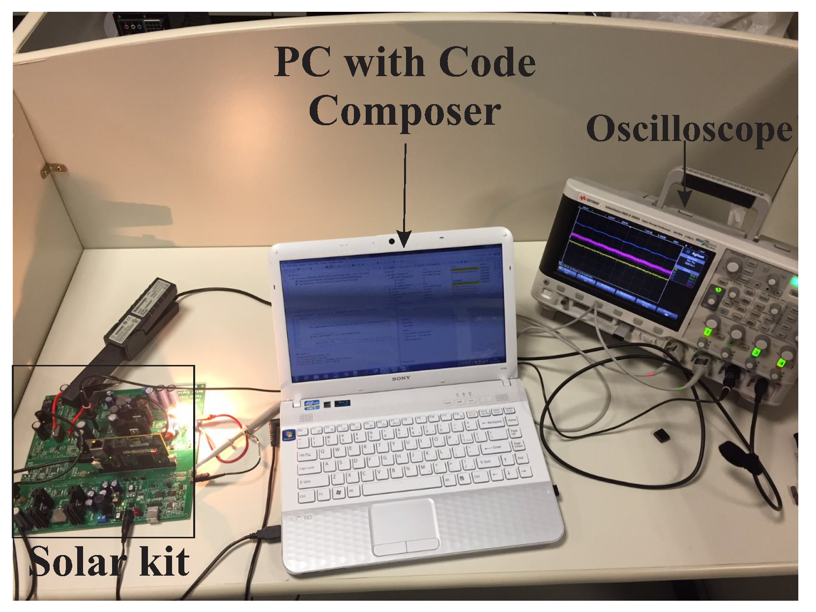
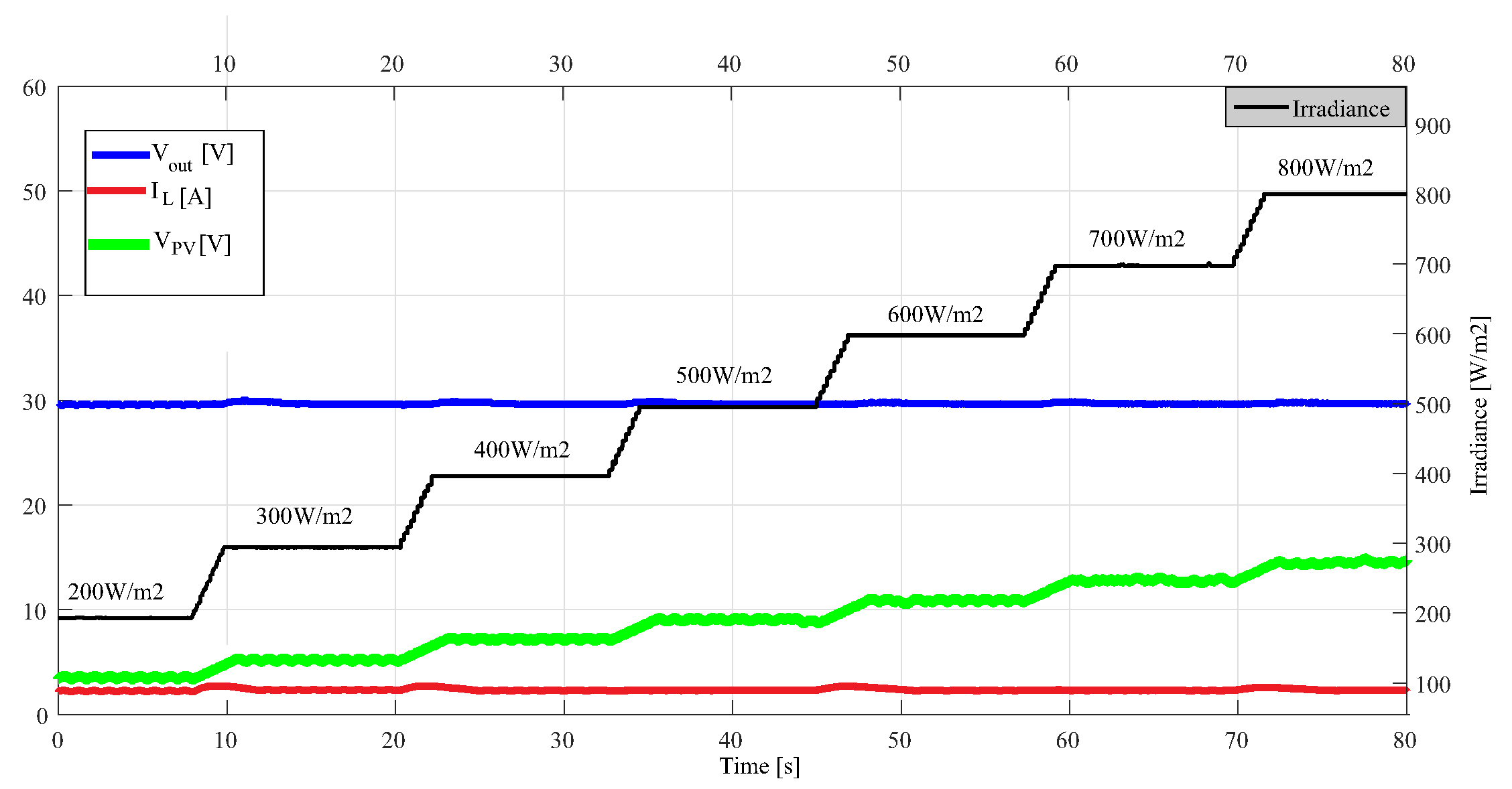
5. Results Using Solar Kit

In order to validate the proposed sliding mode plus PI (SMPI) controller, the Texas instruments Solar Explorer kit (TMDSSOLAR (P/C) EXPKIT) [48] was employed to this task. It is composed of a buck-boost converter, a boost converter, and a full bridge single phase inverter feeding a load of 50 W at the output. The buck-boost converter together with a light sensor are used to emulate voltage versus current curves of a photovoltaic module. On the other hand, the boost converter is used to implement the MPPT so that one allows the control of the input voltage and current of the converter. The single phase inverter controls the output voltage of the boost converter and feeds the resistive load. In Figure 6 the experimental bench is presented. The code composer studio software is used to program the proposed controller.

In this work the performance of the SMPI controller applied to a boost converter in a photovoltaic system is analyzed, for this reason, the AC conversion stage is simplified as a DC source of 30 V in the output of the boost converter. The solar kit can be configured to test each stage of conversion separated from the other which allows checking the control of the current and voltage of the boost converter independently.

The switching frequency of the boost converter is 100 kHz, the value of the inductor is 100 $\mathsf{\mu }$H, the input capacitor has a value of $680.2$ $\mathsf{\mu }$F, and the output capacitor is $0.1$ $\mathsf{\mu }$F. On the other hand, the operating points of the emulator are given in

Table 1. Operating points [48].

Irradiance	${\mathit{P}}_{\mathit{mpp}}$	${\mathit{V}}_{\mathit{mpp}}$	${\mathit{I}}_{\mathit{mpp}}$
1000 W/m${}^2$	$36.02$ W	$18.46$ V	$1.951$ A
900 W/m${}^2$	$32.42$ W	$16.42$ V	$1.974$ A
800 W/m${}^2$	$28.82$ W	$14.68$ V	$1.963$ A
700 W/m${}^2$	$25.22$ W	$12.77$ V	$1.974$ A
600 W/m${}^2$	$21.61$ W	$10.98$ V	$1.968$ A
500 W/m${}^2$	$18.01$ W	$9.093$ V	$1.981$ A
400 W/m${}^2$	$14.41$ W	$7.363$ V	$1.957$ A
300 W/m${}^2$	$10.81$ W	$5.473$ V	$1.975$ A
200 W/m${}^2$	$7.205$ W	$3.67$ V	$1.963$ A

, where the maximum operating power is 36 W.

The parameters of the current and voltage controllers are calculated using the w-PSO algorithm described in the previous section. The values for the current controller are: $k_i=1.0683\times {10}^{-6}$, $k_{pc}=0.2019$, $k_{ic}=498.194$, $Li{m}_{\mathrm{up}}=0.07274$, $Li{m}_{\mathrm{low}}=-0.09519$, and the values for the voltage controller are: $k_v=1.2257\times {10}^{-6}$, $k_{pv}=7$, $k_{iv}=1129$, $Li{m}_{\mathrm{up}}=0.84739$, $Li{m}_{\mathrm{low}}=-1.09229$.

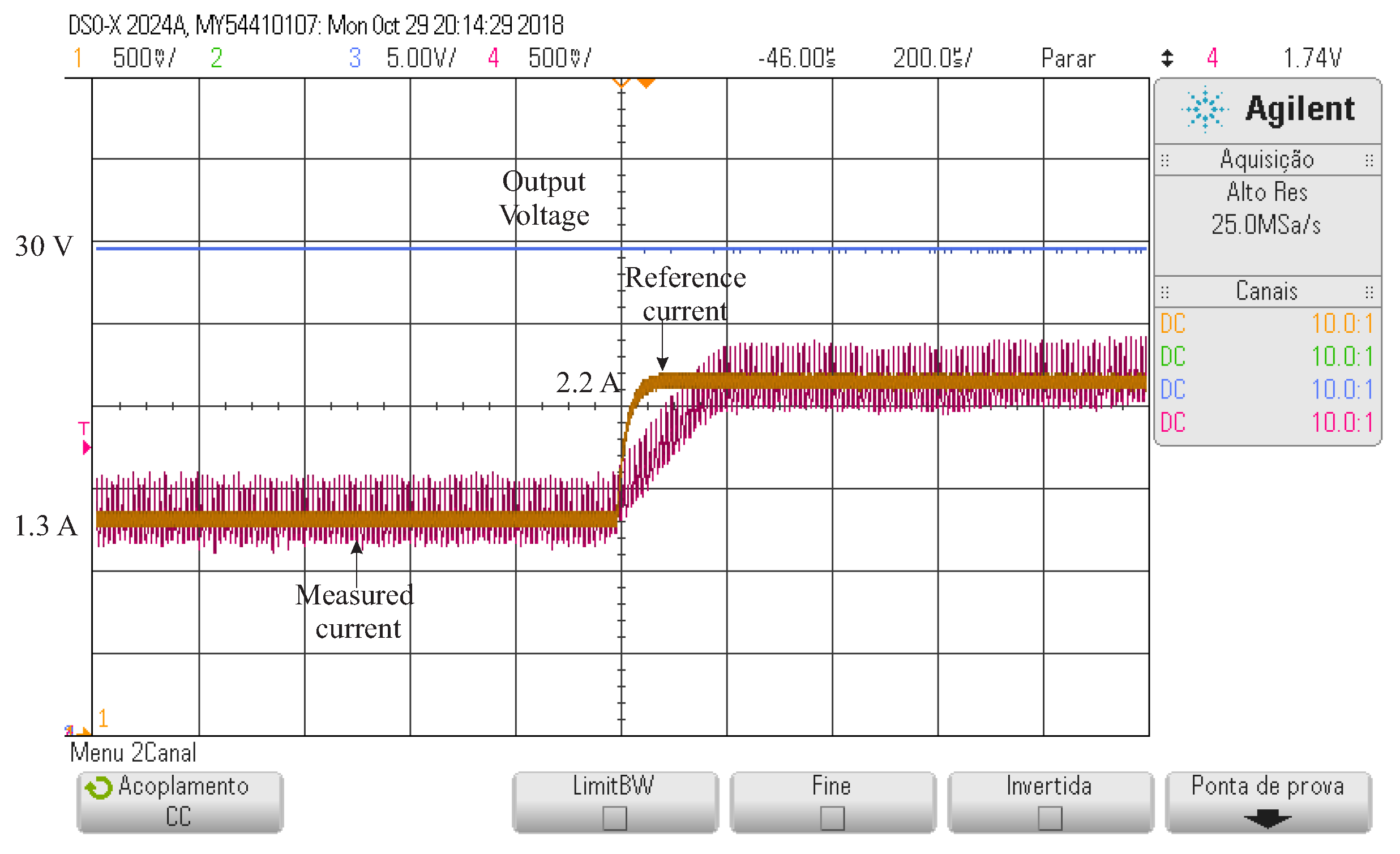
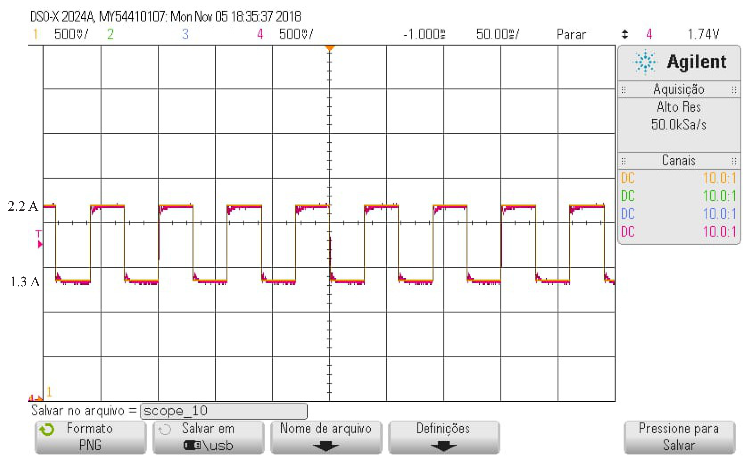
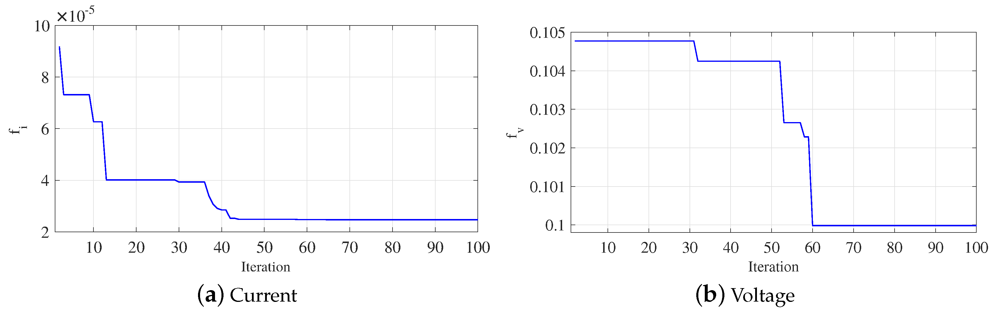
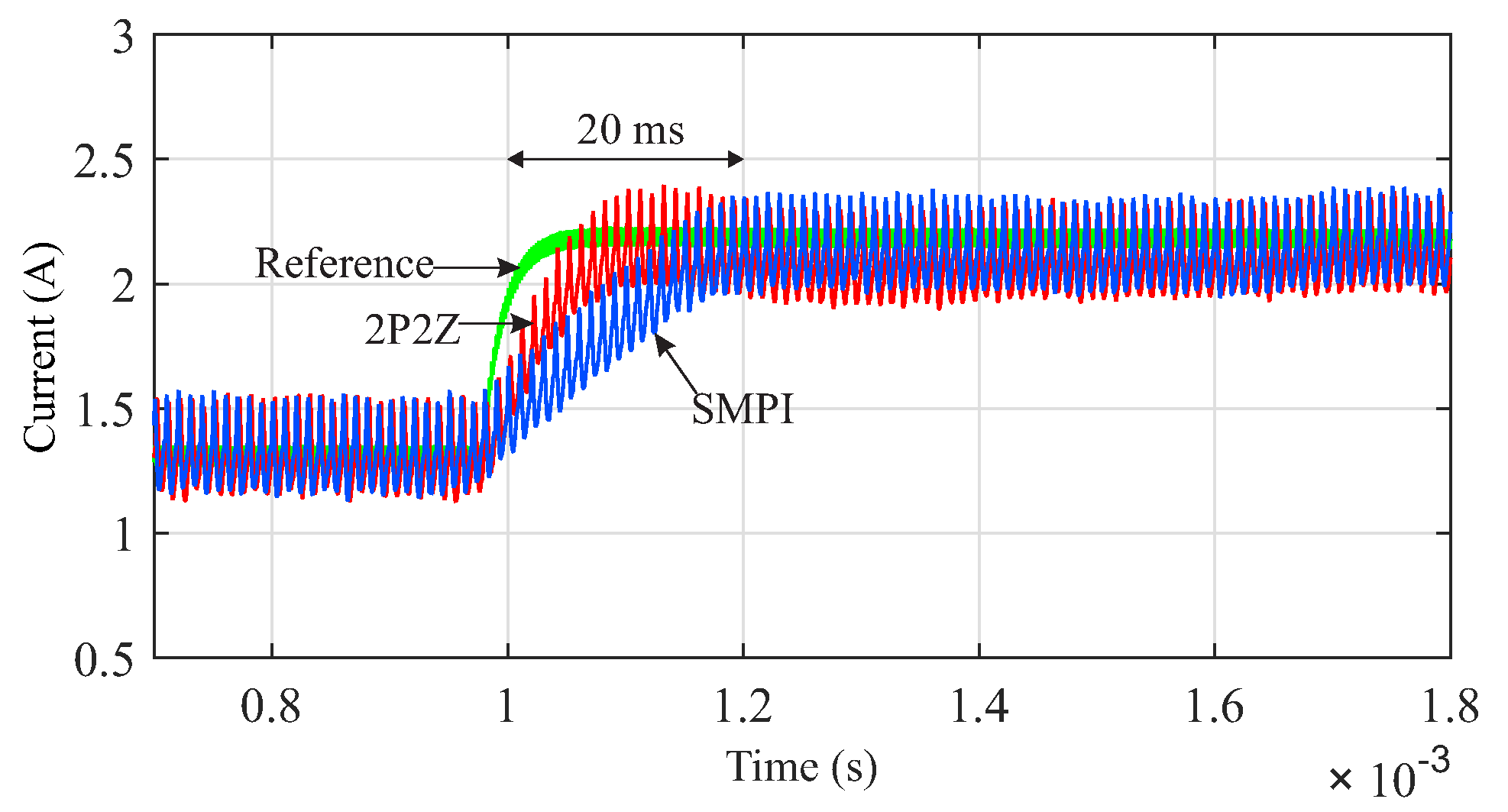
5.1. Current Control

The first test consists in verifying the control of the current by using the SMPI controller. In this case, the step test of the reference current varies from 1.3 A to 2.2 A. Figure 7 depicts the performance of the proposal in which the settling time is about 200 $\mathsf{\mu }$s without overshoot. In addition to the current, the figure also shows the output voltage of the converter that is maintained at a value of 30 V.

Figure 8 shows a square reference profile from 1.3 A to 2.3 A to verify the current response of the SMPI controller. It can be observed that the controller proposed reaches the current references and the output voltage is kept constant at 30 V.

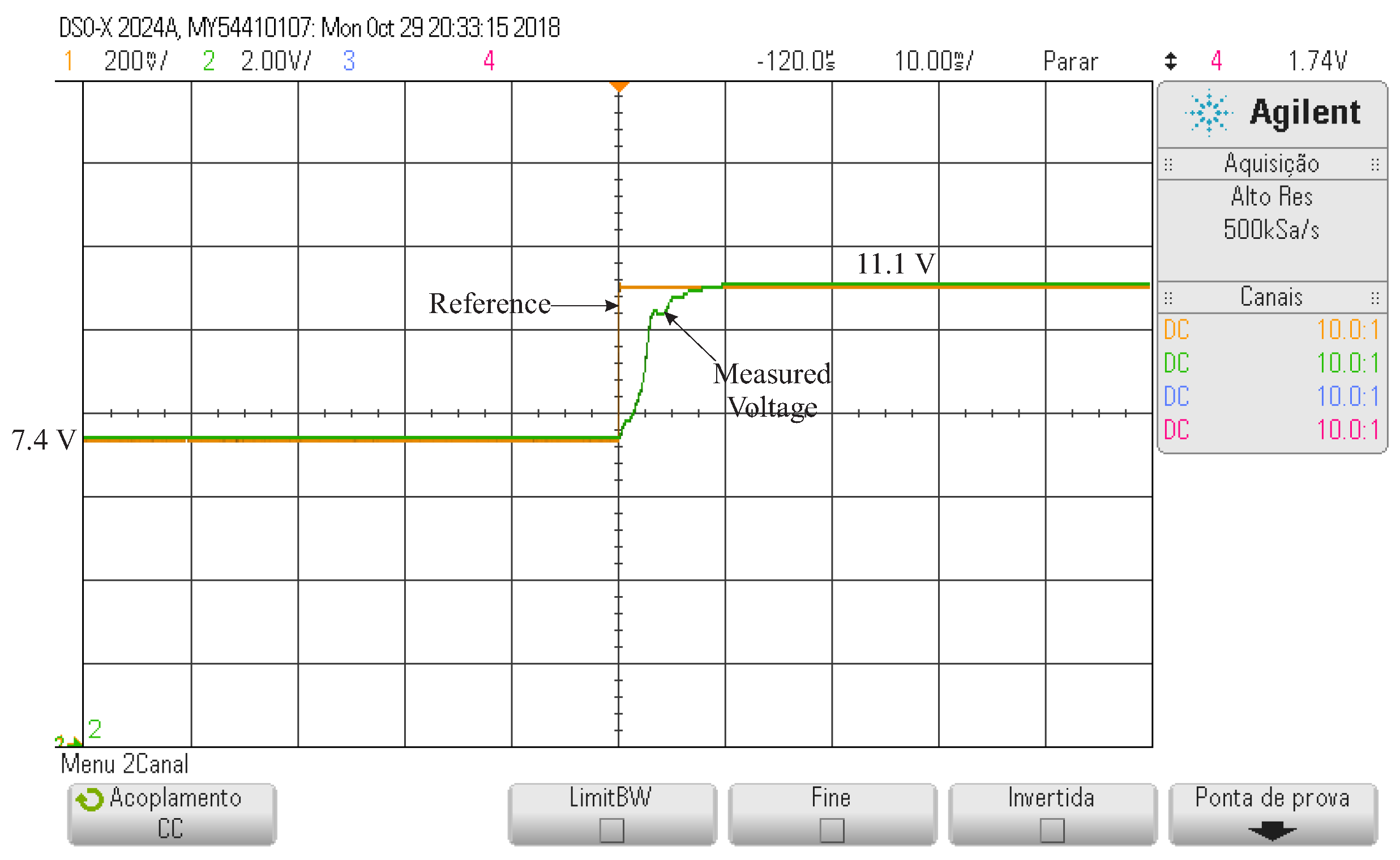
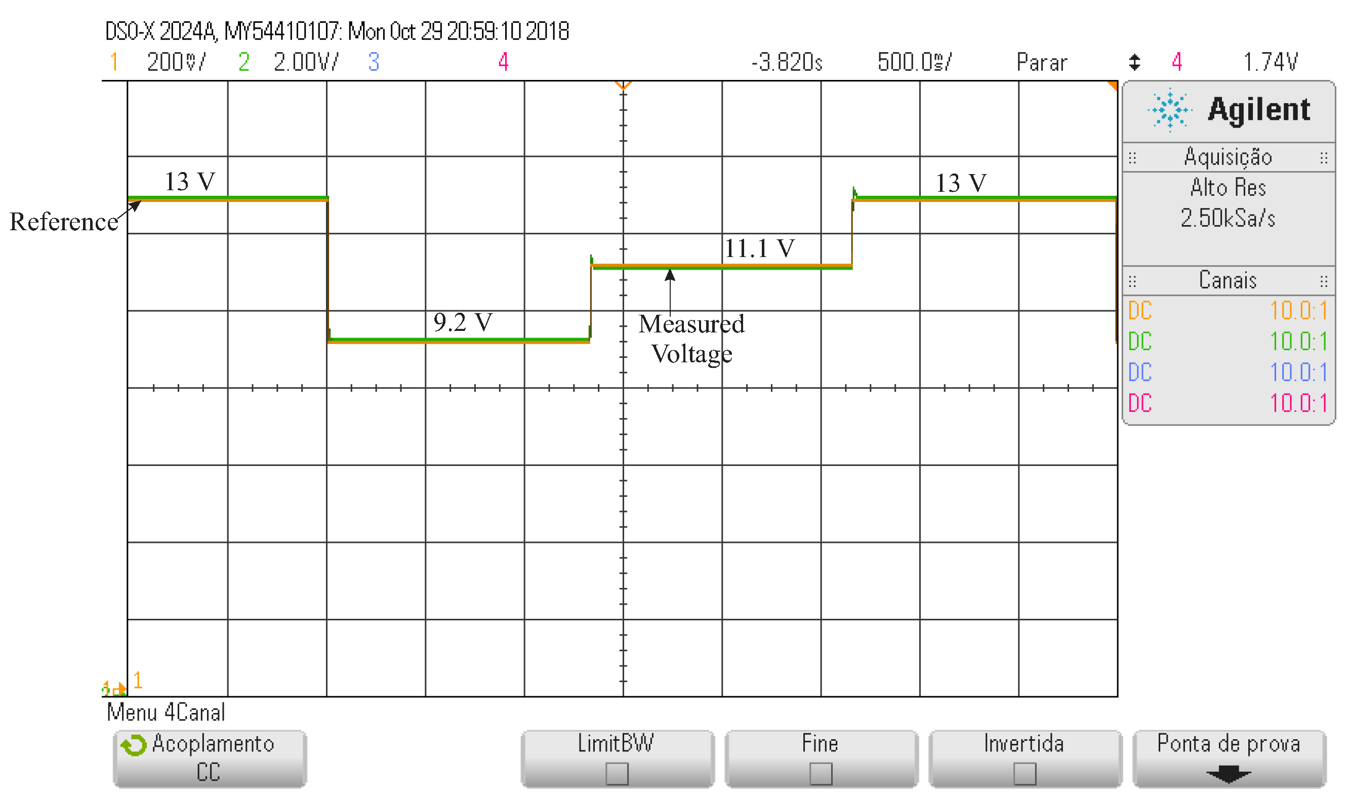
5.2. Voltage Control

Once the current controller is verified, the next step is to test the voltage control. For this test, a square voltage profile of reference that starts at 13 V, decreases to 9.2 V, then increases to 11.1 V and ends at 13 V again was implemented. The performance of the proposal is depicted in Figure 9. It can be noticed that the proposed SMPI reaches the voltage references without steady state error.

A step voltage test in which the voltage varies from 7.4 V to 11.1 V is depicted in Figure 10. It can be noticed the satisfactory performance of the proposal due to the measured voltage stabilizes in 8 ms, without overshoot and oscillations in steady state.

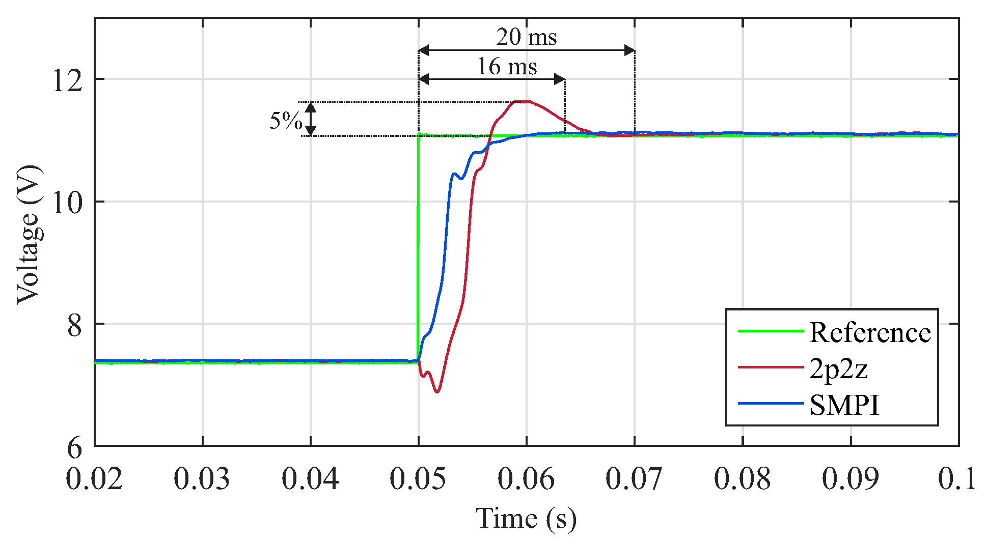
5.3. Comparison Performance Tests

One way to check the performance of the proposed controller is to compare its response with another type of controller, such as a linear controller. To project linear controllers it is necessary to calculate the transfer function of the plant at a specific point of operation and use some classic control technique as a response in frequency. Within this category are the PI, PID, and lead-leg. Therefore, in this work a two-pole two-zero controller (2p2z) [49], which corresponds to a lead-leag controller, was projected using the procedure described in [10]. The design criteria of the 2p2z controller are: crossover frequency is 10 kHz and the phase margin is 70 degrees for current loop, and crossover frequency is 1500 Hz and the phase margin is 90 degrees for voltage loop.

The response for a current step test by using the proposed SMPI controller and the 2p2z controller are presented in Figure 11. It is noticed that both controllers have the same settling time about 0.2 ms and the SMPI has no overshoot.

On the other hand, the test for a voltage step by using the 2p2z controller and the proposed SMPI controller are presented in Figure 12. The superior performance of the proposal can be seen due to the response using the 2p2z controller has an overshoot of 5%, while the response using sliding modes is 0.36%. In addition, the settling time for the 2p2z controller is greater than the settling time for sliding modes being 20 ms and 16 ms, respectively.

Once the control loops have been verified, the next test consists in analyzing the performance of the controllers in the presence of a stepped irradiation profile. As shown in Figure 13, the solar irradiation level starts from 200 W/m${}^2$, then increases to 300 W/m${}^2$, and continues increasing in steps of 100 W/m${}^2$ to reach 800 W/m${}^2$. To calculate the value of the reference voltage, the MPPT algorithm incremental conductance is used [50]. The results obtained show that the $V_{pv}$ perfectly tracks the $V_{MPPT}$ reference given by the MPPT. In addition, at each irradiance level, the voltage $V_{MPPT}$ specified in Table 1 is obtained. The $I_L$ current also perfectly tracks the reference $I_{Lref}$. Likewise, the output voltage $V_{out}$ is 30 V at all times.

6. Conclusions

This paper presents a new controller to regulate the voltage and current of a boost converter in a photovoltaic system. In spite of belonging to the non-linear controllers group, the proposed controller is simple and only requires the adjustment of few parameters. This controller is also characterized by operating with constant switching frequency and by using pulse width modulation to calculate the control pulses of the converter switch, which eliminates the problem related to the losses due to high switching frequencies. The proposed controller also allows one to improve the response, obtaining lower overshoot and settling time when compared to the response of a linear lead-leg controller.

The parameters of the proposed controller are calculated using the modified w-PSO algorithm. The adjustment in the calculation of the inertial weight and the use of a secondary objective function allow us to improve the search of the PSO and find an optimal solution quickly and reliably. Results confirm the improvement in the performance of the proposed controller.

References

1. Chatrenour, N.; Razmi, H.; Doagou-Mojarrad, H. Improved double integral sliding mode MPPT controller based parameter estimation for a stand-alone photovoltaic system. Energy Convers. Manag. 2017, 139, 97–109. [Google Scholar] [CrossRef]
2. Karami, N.; Moubayed, N.; Outbib, R. General review and classification of different MPPT Techniques. Renew. Sustain. Energy Rev. 2017, 68, 1–18. [Google Scholar] [CrossRef]
3. De Brito, M.A.G.; Galotto, L.; Sampaio, L.P.; de Azevedo e Melo, G.; Canesin, C.A. Evaluation of the Main MPPT Techniques for Photovoltaic Applications. IEEE Trans. Ind. Electron. 2013, 60, 1156–1167. [Google Scholar] [CrossRef]
4. Adly, M.; El-Sherif, H.; Ibrahim, M. Maximum power point tracker for a PV cell using a fuzzy agent adapted by the fractional open circuit voltage technique. In Proceedings of the 2011 IEEE International Conference on Fuzzy Systems (FUZZ-IEEE 2011), Taipei, Taiwan, 27–30 June 2011; pp. 1918–1922. [Google Scholar] [CrossRef]
5. Nedumgatt, J.J.; Jayakrishnan, K.B.; Umashankar, S.; Vijayakumar, D.; Kothari, D.P. Perturb and observe MPPT algorithm for solar PV systems-modeling and simulation. In Proceedings of the 2011 Annual IEEE India Conference, Hyderabad, India, 16–18 December 2011; pp. 1–6. [Google Scholar] [CrossRef]
6. Tey, K.S.; Mekhilef, S. Modified incremental conductance MPPT algorithm to mitigate inaccurate responses under fast-changing solar irradiation level. Sol. Energy 2014, 101, 333–342. [Google Scholar] [CrossRef]
7. Algazar, M.M.; L-monier, H.A.; L-halim, H.A.E.; Salem, E.E.K. Maximum power point tracking using fuzzy logic control. Int. J. Electr. Power Energy Syst. 2012, 39, 21–28. [Google Scholar] [CrossRef]
8. Messalti, S.; Harrag, A.; Loukriz, A. A new variable step size neural networks MPPT controller: Review, simulation and hardware implementation. Renew. Sustain. Energy Rev. 2017, 68, 221–233. [Google Scholar] [CrossRef]
9. Villalva, M.G.; Siqueira, T.G.D.; Ruppert, E. Voltage regulation of photovoltaic arrays: Small-signal analysis and control design. IET Power Electron. 2010, 3, 869–880. [Google Scholar] [CrossRef]
10. Gil, G.M.V.; Catata, E.O.H.; Ccarita, J.C.C.; Cardoso, J.G.; Filho, A.J.S.; Azcue-Puma, J.L. Digital controller design for interleaved boost converter in photovoltaic system. In Proceedings of the 2016 12th IEEE International Conference on Industry Applications (INDUSCON), Curitiba, Brazil, 20–23 November 2016; pp. 1–8. [Google Scholar]
11. Elgendy, M.A.; Zahawi, B.; Atkinson, D.J. Assessment of Perturb and Observe MPPT Algorithm Implementation Techniques for PV Pumping Applications. IEEE Trans. Sustain. Energy 2012, 3, 21–33. [Google Scholar] [CrossRef]
12. Mohamed, H.A.; Khattab, H.A.; Mobarka, A.; Morsy, G.A. Design, control and performance analysis of DC-DC boost converter for stand-alone PV system. In Proceedings of the 2016 Eighteenth International Middle East Power Systems Conference (MEPCON), Cairo, Egypt, 27–29 December 2016; pp. 101–106. [Google Scholar]
13. Li, C.-H.; Zhu, X.-J.; Cao, G.-Y.; Hu, W.-Q.; Sui, S.; Hu, M.-R. A maximum power point tracker for photovoltaic energy systems based on fuzzy neural networks. J. Zhejiang Univ.-Sci. A 2009, 10, 263–270. [Google Scholar] [CrossRef]
14. Kumar, N.; Saha, T.K.; Dey, J. Sliding-Mode Control of PWM Dual Inverter-Based Grid-Connected PV System: Modeling and Performance Analysis. IEEE J. Emerg. Sel. Top. Power Electron. 2016, 4, 435–444. [Google Scholar] [CrossRef]
15. Pradhan, R.; Subudhi, B. Double Integral Sliding Mode MPPT Control of a Photovoltaic System. IEEE Trans. Control Syst. Technol. 2016, 24, 285–292. [Google Scholar] [CrossRef]
16. Mamarelis, E.; Petrone, G.; Spagnuolo, G. Design of a Sliding-Mode-Controlled SEPIC for PV MPPT Applications. IEEE Trans. Ind. Electron. 2014, 61, 3387–3398. [Google Scholar] [CrossRef]
17. Montoya, D.G.; Ramos-Paja, C.A.; Giral, R. Improved Design of Sliding-Mode Controllers Based on the Requirements of MPPT Techniques. IEEE Trans. Power Electron. 2016, 31, 235–247. [Google Scholar] [CrossRef]
18. Dahech, K.; Allouche, M.; Damak, T.; Tadeo, F. Backstepping sliding mode control for maximum power point tracking of a photovoltaic system. Electric Power Syst. Res. 2017, 143, 182–188. [Google Scholar] [CrossRef]
19. Trindade, F.S.; Filho, A.J.S.; Jacomini, R.V.; Ruppert, E. Experimental results of sliding-mode power control for doubly-fed induction generator. In Proceedings of the 2013 Brazilian Power Electronics Conference, Gramado, Brazil, 27–31 October 2013; pp. 686–691. [Google Scholar]
20. Lascu, C.; Boldea, I.; Blaabjerg, F. Direct torque control of sensorless induction motor drives: A sliding-mode approach. IEEE Trans. Ind. Appl. 2004, 40, 582–590. [Google Scholar] [CrossRef]
21. Anantwar, H.; Lakshmikantha, D.B.R.; Sundar, S. Fuzzy self tuning PI controller based inverter control for voltage regulation in off-grid hybrid power system. Energy Procedia 2017, 117, 409–416. [Google Scholar] [CrossRef]
22. Kihal, A.; Krim, F.; Laib, A.; Talbi, B.; Afghoul, H. An improved MPPT scheme employing adaptive integral derivative sliding mode control for photovoltaic systems under fast irradiation changes. ISA Trans. 2018. [Google Scholar] [CrossRef] [PubMed]
23. Khazane, J.E.; Tissir, E.H. Achievement of MPPT by finite time convergence sliding mode control for photovoltaic pumping system. Sol. Energy 2018, 166, 13–20. [Google Scholar] [CrossRef]
24. Kchaou, A.; Naamane, A.; Koubaa, Y.; M’sirdi, N. Second order sliding mode-based MPPT control for photovoltaic applications. Sol. Energy 2017, 155, 758–769. [Google Scholar] [CrossRef]
25. Bounar, N.; Labdai, S.; Boulkroune, A. PSO-GSA based fuzzy sliding mode controller for DFIG-based wind turbine. ISA Trans. 2018, 85, 177–188. [Google Scholar] [CrossRef] [PubMed]
26. Liu, H.; Sung, W.; Yao, W. Computer, Intelligent Computing and Education Technology; CRC Press: Hong Kong, China, 2014; Volume 1. [Google Scholar]
27. Gavhane, P.S.; Krishnamurthy, S.; Dixit, R.; Ram, J.P.; Rajasekar, N. EL-PSO based MPPT for Solar PV under Partial Shaded Condition. Energy Procedia 2017, 117, 1047–1053. [Google Scholar] [CrossRef]
28. Eswaran, T.; Kumar, V.S. Particle swarm optimization (PSO)-based tuning technique for PI controller for management of a distributed static synchronous compensator (DSTATCOM) for improved dynamic response and power quality. J. Appl. Res. Technol. 2017, 15, 173–189. [Google Scholar] [CrossRef]
29. Ruiz-Cruz, R.; Sanchez, E.N.; Ornelas-Tellez, F.; Loukianov, A.G.; Harley, R.G. Particle Swarm Optimization for Discrete-Time Inverse Optimal Control of a Doubly Fed Induction Generator. Energies 2014, 7, 1706–1720. [Google Scholar] [CrossRef] [PubMed]
30. Chen, J.-H.; Yau, H.-T.; Hung, W. Design and study on sliding mode extremum seeking control of thechaos embedded particle swarm optimization for maximum power point tracking in wind power systems. IEEE Trans. Cybern. 2013, 43, 1698–1709. [Google Scholar]
31. Kessentini, S.; Barchies, D. Particle swarm optimization with adaptive inertia weight. Int. J. Mach. Learn. Comput. 2015, 5, 368–373. [Google Scholar] [CrossRef]
32. Villalva, M.G.; Ruppert, F.E. Analysis and simulation of the P&O MPPT algorithm using a linearized PV array model. In Proceedings of the 2009 35th Annual Conference of IEEE Industrial Electronics, Porto, Portugal, 3–5 November 2009; pp. 231–236. [Google Scholar]
33. Sahu, P.; Verma, D.; Nema, S. Physical design and modelling of boost converter for maximum power point tracking in solar PV systems. In Proceedings of the 2016 International Conference on Electrical Power and Energy Systems (ICEPES), Bhopal, India, 14–16 December 2016; pp. 10–15. [Google Scholar]
34. Ayop, R.; Tan, C.W. Design of boost converter based on maximum power point resistance for photovoltaic applications. Sol. Energy 2018, 160, 322–335. [Google Scholar] [CrossRef]
35. Cucuzzella, M.; Lazzari, R.; Trip, S.; Rosti, S.; Sandroni, C.; Ferrara, A. Sliding mode voltage control of boost converters in DC microgrids. Control Eng. Pract. 2018, 73, 161–170. [Google Scholar] [CrossRef]
36. Yatimi, H.; Aroudam, E. Assessment and control of a photovoltaic energy storage system based on the robust sliding mode MPPT controller. Sol. Energy 2016, 139, 557–568. [Google Scholar] [CrossRef]
37. Mojallizadeh, M.R.; Badamchizadeh, M.; Khanmohammadi, S.; Sabahi, M. Designing a new robust sliding mode controller for maximum power point tracking of photovoltaic cells. Sol. Energy 2016, 132, 538–546. [Google Scholar] [CrossRef]
38. Levant, A. Chattering Analysis. IEEE Trans. Autom. Control 2010, 55, 1380–1389. [Google Scholar] [CrossRef]
39. CSoon, C.; Ghazali, R.; Jaafar, H.I.; Hussien, S.Y.S. Sliding Mode Controller Design with Optimized PID Sliding Surface Using Particle Swarm Algorithm. Procedia Comput. Sci. 2017, 105, 235–239. [Google Scholar] [CrossRef]
40. Vargas-Gil, G.M.; Colque, C.J.C.; Sguarezi, A.J.; Monaro, R.M. Sliding mode plus PI control applied in PV systems control. In Proceedings of the 2017 IEEE 6th International Conference on Renewable Energy Research and Applications (ICRERA), San Diego, CA, USA, 5–8 Nocember 2017; pp. 562–567. [Google Scholar]
41. Yang, M.; Zhang, S. PSO-based PID controller design for unwinding tension system of web press. In Proceedings of the 2018 13th IEEE Conference on Industrial Electronics and Applications (ICIEA), Wuhan, China, 31 May–2 June 2018; pp. 1399–1403. [Google Scholar]
42. Sánchez, J.A. Instrumentación y Control Avanzado de Procesos; Ediciones Díaz de Santos: Madrid, Spain, 2013. [Google Scholar]
43. Lu, H.; Chen, W. Dynamic-objective particle swarm optimization for constrained optimization problems. J. Comb. Optim. 2006, 12, 409–419. [Google Scholar] [CrossRef]
44. Segura, C.; Coello, C.A.; Miranda, G.; León, C. Using multi-objective evolutionary algorithms for single-objective constrained and unconstrained optimization. Ann. Oper. Res. 2016, 240, 217–250. [Google Scholar] [CrossRef]
45. He, F.; Liu, C. Particle Swarm Optimization Applied to a Stochastic Optimization Problem. In Proceedings of the 2010 2nd International Workshop on Database Technology and Applications, Wuhan, China, 27–28 November 2010; pp. 1–4. [Google Scholar]
46. Thangaraj, R.; Pant, M.; Bouvry, P.; Abraham, A. Evolutionary Algorithms for Solving Stochastic Programming Problems. In Proceedings of the 2010 International Conference on Computational Intelligence and Communication Networks, Bhopal, India, 26–28 November 2010; pp. 628–632. [Google Scholar]
47. Žilinskas, A.; Fraga, E.; Mackutė, A. Data analysis and visualisation for robust multi-criteria process optimization. Comput. Chem. Eng. 2006, 30, 1061–1071. [Google Scholar] [CrossRef]
48. Bhardwaj, M.; Subharmanya, B. PV Inverter Design Using Solar Explorer Kit; Texas Instruments: Dallas, TX, USA, 2013. [Google Scholar]
49. Neuman, C.P. The two-pole two-zero root locus. IEEE Trans. Educ. 1994, 37, 369–371. [Google Scholar] [CrossRef]
50. Elgendy, M.A.; Zahawi, B.; Atkinson, D.J. Assessment of the Incremental Conductance Maximum Power Point Tracking Algorithm. IEEE Trans. Sustain. Energy 2013, 4, 108–117. [Google Scholar] [CrossRef]
Figure 1. Block diagram of the system.
Energies 12 00864 g001
Figure 2. Block diagram of the system.
Energies 12 00864 g002
Figure 3. Flowchart of the Particle Swarm Optimization (PSO) algorithm modified.
Energies 12 00864 g003
Figure 4. Evolution of inertial weight.
Energies 12 00864 g004
Figure 5. Evolution of the objective function.
Energies 12 00864 g005
Figure 6. Experimental bench.
Energies 12 00864 g006
Figure 7. Response of the sliding mode plus proportional-integral (SMPI) for a current step test.
Energies 12 00864 g007
Figure 8. Response of the SMPI for a square reference profile of current.
Energies 12 00864 g008
Figure 9. Response of the SMPI for several references values of voltages.
Energies 12 00864 g009
Figure 10. Response of the SMPI for a voltage step test.
Energies 12 00864 g010
Figure 11. Comparison of the SMPI and 2p2z controllers for a current step test.
Energies 12 00864 g011
Figure 12. Comparison of the SMPI and two-pole two-zero controller (2p2z) controllers for a voltage step test.
Energies 12 00864 g012
Figure 13. Irradiation levels and MPPT control.
Energies 12 00864 g013