Hierarchical Multi-Objective Fuzzy Collaborative Optimization of Integrated Energy System under Off-Design Performance

Abstract

In order to solve the frequently occurred nonlinear working characteristics problem of the devices in integrated energy system (IES), where this nonlinear problem causes the offset of operation characteristics and design points of those devices, in this paper, the hierarchical multi-objective fuzzy collaborative optimization model of IES under off-design performance is proposed. Firstly, the high-order nonlinear models of devices under off-design performance, including fuel cell (FC), gas turbine (GT), absorption lithium bromide chiller (ABS), etc., are presented considering renewable energy and diversified storage devices, which can more accurately describe the actual working condition of devices. Secondly, according to the needs of different engineering application modes, the lower level collaborative optimization model of energy hub (EH) with economic, eco-friendly, primary energy saving, and renewable energy accommodation rate as optimization objectives is proposed, which can well adapt to and reflect real world energy system. Thirdly, based on the relationship between master and slave dispatch centers, the upper level modeling and optimal scheduling model of IES consisting of coupling power system, natural gas system, and heat system is proposed. Then, a multi-objective fuzzy collaborative optimization model for EH and IES is developed, where continuous differentiable Sigmoid function is taken as the membership function. Finally, simulation results show that the proposed models and optimal dispatch method can effectively solve the frequently occurred non-linear working characteristics problem of the devices in IES. The optimal results are suitable for planning, calculation, operation, dispatch of IES, which can reasonably reflect the operation characteristics of IES.

1. Introduction

The integrated energy system (IES) has become a vital strategic research direction in international energy field, due to its great significance in improving the comprehensive utilization efficiency of energy, the utilization efficiency of social infrastructure, and the energy supply security [1,2,3]. In addition, the IES also can promote the large-scale development of renewable energy and achieving energy conservation and emissions reduction in China [2,3]. At the same time, the remarkable change of energy production and consumption mode requires changing the construction path and development mode of traditional energy system and constructing IES [4,5,6]. Constructing IES from economic, management and planning perspective is an important part of “building a low-carbon, clean, safe and efficient modern energy system” [6,7].

The IES utilizes the multi-energy flow complementary characteristic, and optimizes energy production, supply and sales lines, which is one of the trends of energy system development in the future [7,8,9]. In the process of discussing modeling methods about IES, the concept of energy hub (EH) proposed by Geidl, Andersson and others has attracted extensive attention from both academia and industry [8,9,10]. In [8], an innovative method was proposed to improve the synergy between the structure optimization and operational optimization of EH, and to enhance the operational performance and reliability of EH. In [9], a multiple energy carriers model coupled different energy was presented based on the new concept of EHs, where combined dispatch and optimal energy flow problems were stated. Based on the EH whose input includes natural gas, electricity, heat, and other energy, and output includes electricity, cooling heat, and other forms of energy, the two layers of optimal scheduling model for IES, and the steady state operation characteristics of each subsystem were analyzed in detail in [10]. In [11], a multi-objective optimization model was proposed for combined cooling, heating and power (CCHP) system, and the coupling relationship of various energy within CCHP was also analyzed, for maximizing energy saving efficiency of devices including absorption chiller and electric chiller, and minimizing the energy cost of CCHP system. In [12], a new sub-EH modeling structure consisted of heat hub, electricity hub, and cold hub was proposed, which took into account energy storage devices, such as electricity, cold and heat energy storage, realizing energy collection, distribution and storage of energy. However, in the above mentioned work, the multi-input and multi-output relationships of EH are generally reduced to linear coupling relationships [2,5]. In fact, devices usually have non-linear working characteristics which means deviation from the design performance [5,6]. The neglect or simplification of each device’s off-design characteristics by linear EH model makes energy conversion relationship and transfer result of EH unacceptable [3,7].

With the increasing of key devices in IES, the deepening of energy coupling and the diversification of load demand, IES is mainly faced with the following problems in modeling [1,10]. The issue of analyzing the energy conversion, storage and distribution of IES under the conditions of retaining the main characteristics of different energies and meeting the energies balance in the face of complex energy systems with multi-level difference and multi-space-time difference [6,12]. In [6], a hierarchical optimization model based on an extended EH was proposed for small and medium-sized regional IES with flexible operation methods, then a bi-level optimization model with the lower comprehensive energy cost and the higher energy efficiency was developed. However, the inter-system coupling devices unit involved are too simple, so that there are some difficulties in engineering application [7,9]. From the perspective of master and slave dispatch center, a hierarchical optimal scheduling model was presented for IES coupling power distribution system, natural gas transmission system and heat distribution system in [10]. It focuses on each subsystem without considering the devices’ physical constraints such as load rate, start-up time, working hours and off-design performance in detail. Taking the IES as the participant of the regulation market, the optimization model of IES based on pay-for-performance was proposed in [13]. However, it should be pointed out that the so-called IES in the above mentioned results only stays on the basis of energy flow and does not really involve subsystems with key characteristic variables. The above “subsystem degree” research on IES is not deep enough on the whole or the system level, especially in the IES problem involving hierarchical multi-objective optimal operation and cooperative optimal scheduling of natural gas, power, and heat system. It can be seen that problem of IES collaborative optimization under off-design performance still needs to be further studied.

Based on the above analysis, in this paper, the hierarchical multi-objective fuzzy collaborative optimization model of IES under different operating conditions is proposed to solve the nonlinear working characteristics problem of the devices in IES, where this nonlinear problem causes the offset of operation characteristics and design points of those devices. The proposed model and optimization method considering off-design performance of devices provides the basis for planning, calculation and optimized operation analysis of IES. Motivated by the mentioned issues, the main contributions of this paper are summarized as follows:

(1)

High-order nonlinear models of devices under off-design performance are developed considering renewable energy and diversified storage devices.

(2)

EH under off-design performance is introduced based on geographical resource endowment, then, a lower level multi-objective collaborative optimization model for such case is proposed.

(3)

Upper level modeling and multiple optimal scheduling modes of IES with the coupling and interactions between heat system, power system, and natural gas system, are proposed, fully considering the key characteristic variables of the energy subsystems.

(4)

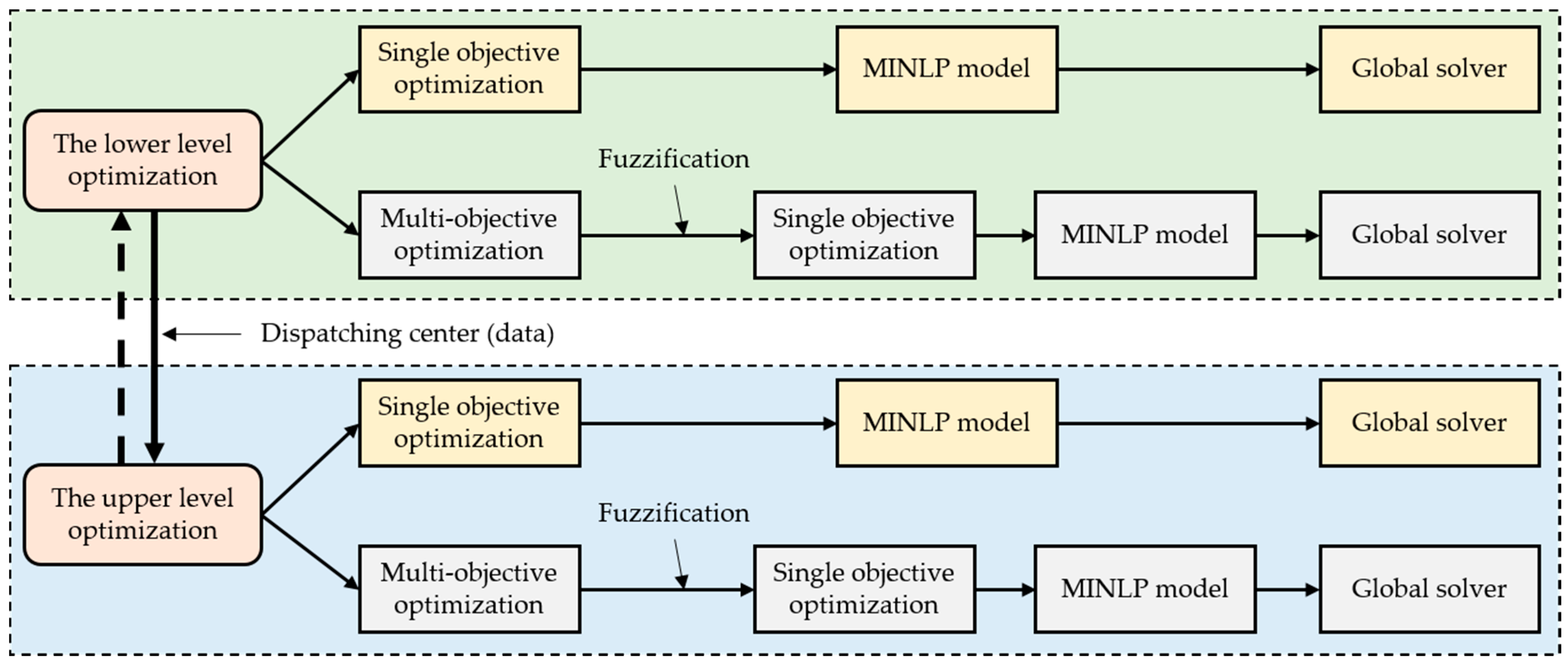
A hierarchical multi-objective collaborative optimization model for EH and IES is developed, facing engineering application modes and based on the relationship between master and slave dispatch centers.

(5)

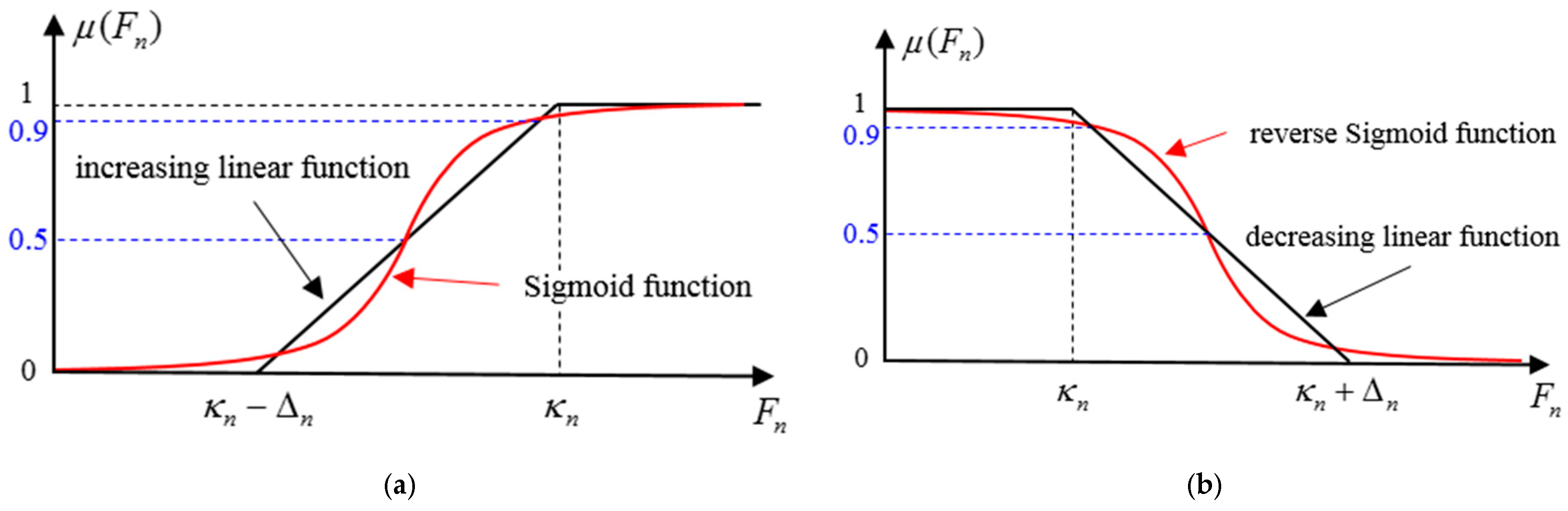
An improved multi-objective fuzzy optimization method is presented, where continuous differentiable Sigmoid function is introduced as an improved membership function.

2. Lower Level Modeling and Optimization

EH is defined as an input-output port model that describes the exchange and coupling relationship between source, load, storage, and network in IES. The EHs are a sub-part of the IES, where the EH is an equivalent multi-energy demand load terminal of IES. EH can act as a mutual conversion, distribution, consumption, and storage of all kinds of energy, with a strong flexibility [6,8,10].

2.1. Energy Device Unit Model of Energy Hub under Off-Design Performance

The main frame model of EH is relatively mature, and the detailed understanding can be referred to [10,14,15,16]. Next, this paper mainly introduces the key devices model under off-design performance in EH.

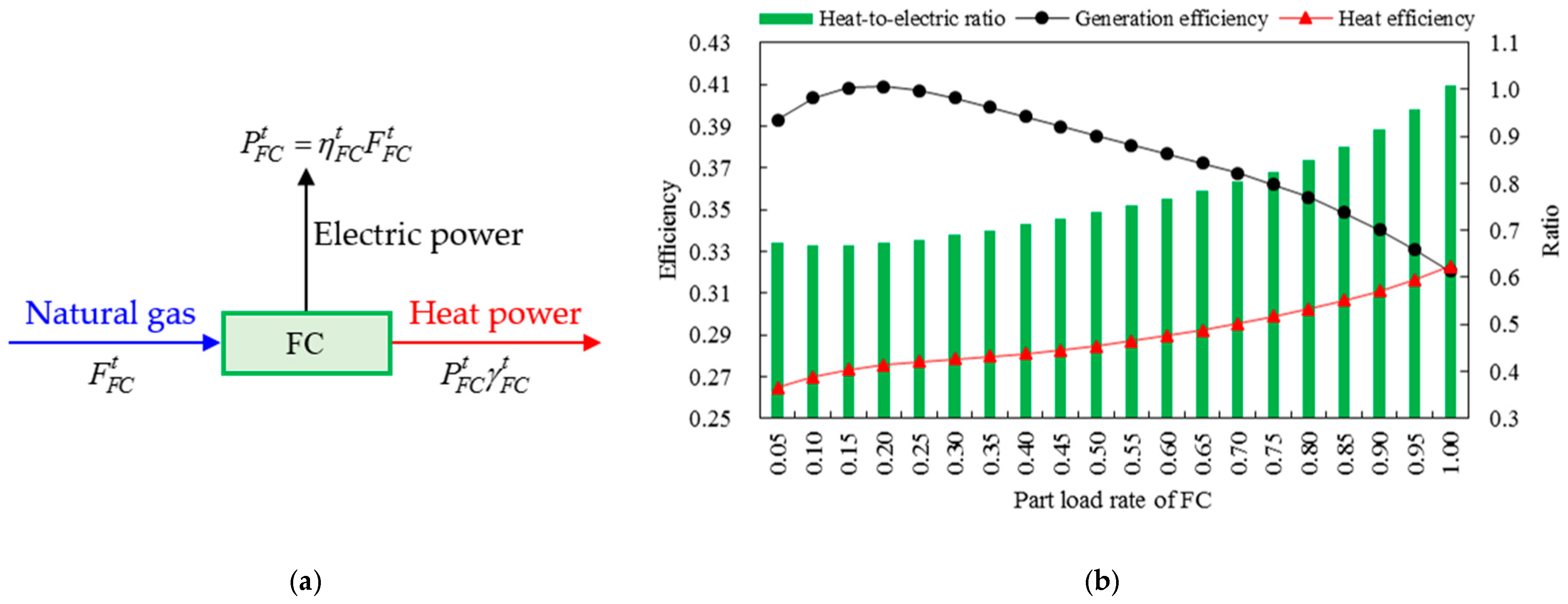
2.1.1. Fuel Cell (FC)

FC is a kind of power generation and heat generation device that directly converts the chemical energy of fuel into electric energy. That chemical energy of hydrocarbon fuel such as natural gas and hydrogen is directly converted into electric energy through electrochemical reaction, where its load response is fast and the operation quality is high. FC can also achieve good coupling and complementarity with GT and power generation system, and form a multi-energy flow supply system. It follows from [12,17] that the FC model under off-design performance is shown as:

$$\{\begin{array}{c}{P}_{FC}^t={\eta }_{FC}^t{F}_{FC}^t\\ {\eta }_{FC}^t={\phi }_{\eta }\left(P_{FC}^t\right)={\displaystyle \sum _{n=0}^5{a}_n{\left({\tilde{P}}_{FC}^t\right)}^n}{X}_{FC}^t\\ {\gamma }_{FC}^t={\phi }_{\gamma }\left(P_{FC}^t\right)={\displaystyle \sum _{n=0}^4{b}_n{\left({\tilde{P}}_{FC}^t\right)}^n}{X}_{FC}^t\end{array}$$

(1)

where ${\eta }_{FC}^t$ and ${\gamma }_{FC}^t$ denote the generation efficiency and heat-to-electric ratio of FC at time $t$, respectively. ${\phi }_{\eta }(\cdot )$ is the mathematical functional relation. $a_n$ and $b_n$ are the constant coefficients of the $n$th power item in different functions. $F_{FC}^t$, $P_{FC}^t$ and ${\tilde{P}}_{FC}^t$ represent the input fuel amount, output electric power and part load rate of FC at time $t$, respectively. $X_{FC}^t$ is the binary-variable of FC operation state, with 1 for run and 0 for shutdown.

The established FC model above has extensive universality. A typical FC case under off-design performance is shown in Figure 1, in which the data is from the reference [17]. As can be seen in Figure 1, the generation efficiency and heat efficiency of FC is changing under different part load rates. Obviously, a large error will be produced by using the modeling method of the constant generation efficiency without considering the off-design performance characteristics.

2.1.2. Gas Turbine (GT)

Regarding GT as the main energy supply equipment of the multi-energy flow system with coupling natural gas, electricity and heat, its operation efficiency varies greatly under part load rates [10,14]. The third-order generation efficiency function is used to fit the model [18], the GT model under variable operating conditions is given by:

$$\{\begin{array}{c}{P}_{GT}^t={\eta }_{GT}^t{F}_{GT}^t\\ H_{GT}^t{\eta }_{GT}^t=P_{GT}^t\left(1-{\eta }_{GT}^t-{\eta }_{loss}\right)\\ {\eta }_{GT}^t={\phi }_{\eta }\left(P_{GT}^t\right)={\displaystyle \sum _{n=0}^3{c}_n{\left({\tilde{P}}_{GT}^t\right)}^n}{X}_{GT}^t\end{array}$$

(2)

where $F_{GT}^t$, $P_{GT}^t$, ${\tilde{P}}_{GT}^t$ and $H_{GT}^t$ are the input fuel amount, output electric power, part load rate and output thermal power of GT at time $t$, respectively. ${\eta }_{GT}^t$ and ${\eta }_{loss}$ represent the generation efficiency and heat loss rate of GT at time $t$, respectively. $c_n$ is the constant coefficient of the $n$th power item for GT model. $X_{GT}^t$ denotes the binary-variable of GT operation state, with 1 for run and 0 for shutdown.

2.1.3. Waste Heat Recovery System (REC)

REC centralizes recovery of waste heat generated by GT and FC to achieve further EH energy utilization efficiency [18,19]. Common REC is mainly composed of regenerators, or absorption refrigeration equipment, or heat exchangers, etc. The heat energy output by REC is related to the heat recovery efficiency, which is also affected by the part load rate, which can be expressed by:

$$\{\begin{array}{c}{H}_{REC}^t={\eta }_{REC}^t{F}_{REC}^t\\ {\eta }_{REC}^t={\phi }_{\eta }\left(H_{REC}^t\right)={\displaystyle \sum _{n=0}^3{d}_n{\left({\tilde{H}}_{REC}^t\right)}^n}{X}_{REC}^t\end{array}$$

(3)

where $F_{REC}^t$, $H_{REC}^t$ and ${\tilde{H}}_{REC}^t$ are the input waste heat power, output heat power, and part load rate of REC at time $t$, respectively. ${\eta }_{REC}^t$ is the heat recovery efficiency of REC at time $t$. $d_n$ represents the constant coefficient of the $n$th power item for REC model. $X_{REC}^t$ denotes the binary-variable of REC operation state, with 1 for run and 0 for shutdown.

2.1.4. Gas Boiler (GB)

GB is usually used as the heat source of EH to provide or supplement heat energy, and its working characteristics are relatively stable. The heat generated by GB is related to the heating efficiency of boiler, it follows from [18,19,20] that the second-order variable working condition characteristic model of GB is formulated as:

$$\{\begin{array}{c}{H}_{GB}^t={\eta }_{GB}^t{F}_{GB}^t\\ {\eta }_{GB}^t={\phi }_{\eta }\left(H_{GB}^t\right)={\displaystyle \sum _{n=0}^2{e}_n{\left({\tilde{H}}_{GB}^t\right)}^n}{X}_{GB}^t\end{array}$$

(4)

where $F_{GB}^t$, $H_{GB}^t$ and ${\tilde{H}}_{FC}^t$ are the input waste heat power or fuel amount, output heat power, and part load rate of GB at time $t$, respectively. ${\eta }_{GB}^t$ represents heating efficiency of GB at time $t$. $e_n$ is the constant coefficient of the $n$th power item for GB model. $X_{GB}^t$ denotes the binary-variable of GB operation state, with 1 for run and 0 for shutdown.

2.1.5. Ground Source Heat Pump (GSHP)

GSHP usually takes shallow geothermal resources as the heat source, which has the advantages of energy saving, environmental protection and convenient regulation. It can be used for heating in winter and cooling in summer [10,18]. Compared to traditional heating methods that can only convert a small part of the electrical energy into heat energy, which is not economic, GSHP’s output (thermoelectric or cold energy), by absorbing low temperature heat from the environment or releasing heat energy into the environment, can be relatively high with only consuming small amount of electric power as an input, thereby significantly reducing fossil energy consumption [18,21]. However, its working time pattern is usually limited for reducing damage to the energy balance of the environment, thus GSHP works as follows:

$$\{\begin{array}{c}{H}_{GSHP}^t=CO{P}_{GSHP}^t{P}_{GSHP}^t{X}_{GSHP}^t\\ CO{P}_{GSHP}^t={\phi }_{\eta }\left(T^{tem}\right)+{\phi }_{\eta }\left(H_{GSHP}^t\right)=f_0+f_1{T}_{ev}^{tem}+f_2{T}_{cd}^{tem}+{\displaystyle \sum _{n=0}^2{g}_n{\left({\tilde{H}}_{GSHP}^t\right)}^n}{X}_{GSHP}^t\\ {\displaystyle \sum _{t=T_{start}}^{T_{end}}t{X}_{GSHP}^t}\le {\epsilon }_{acc}T\end{array}$$

(5)

where $P_{GSHP}^t$, $H_{GSHP}^t$, and ${\tilde{H}}_{GSHP}^t$ are the input electrical power, output heat power, and part load rate of GSHP at time $t$, respectively. $CO{P}_{GSHP}^t$ denotes coefficient of performance of GSHP at time $t$. $T_{ev}^{tem}$ is the average water temperature at the inlet and outlet of evaporator. $T_{cd}^{tem}$ denotes the average water temperature at the inlet and outlet of the condenser. $T_{ev}^{tem}$ and $T_{cd}^{tem}$ are affected by seasonal climate and environmental temperature, therefore, for the sake of simplicity, and this paper does not model temperature changes and sets them as given the variables. $f_0\sim f_2$ are the temperature fitting constant coefficients. $g_n$ denotes the constant coefficient of the n-th power item for GSHP model. $X_{GSHP}^t$ is the binary-variable of GSHP operation state, with 1 for run and 0 for shutdown. $T_{start}$ and $T_{end}$ are the starting and ending time of GSHP’s working period, respectively. ${\epsilon }_{acc}$ denotes the ratio of the maximum working time of GSHP in the optimized scheduling cycle $T$.

2.1.6. Micro-Gas Turbine (MT)

MT can use natural gas, biogas and other fuels for power generation and heating. Generally, the generating efficiency of MT is improved with the increase of power generation, and reaches the maximum efficiency at the rated load [17]. The load characteristics of MT describe the relationship between the equipment efficiency, smoke discharge temperature, smoke discharge flow rate and other parameters when the output power changes at a constant speed. It follows from [18,22] that the relationship can be expressed by the following equations in the case of capacity determination:

$$\{\begin{array}{c}{P}_{MT}^t={\eta }_{MT}^{e,t}{F}_{MT}^t\\ {\eta }_{MT}^t=\left(h_0{C}_{MT}+h_1{\tilde{P}}_{MT}^t+h_2{C}_{MT}{\tilde{P}}_{MT}^t+h_3\right)X_{MT}^t\\ {\tilde{T}}_{MT}^{tem,t}={\phi }_{\eta }\left(P_{MT}^t\right)={\displaystyle \sum _{n=0}^3{j}_n{\left({\tilde{P}}_{MT}^t\right)}^n}{X}_{MT}^t\\ {\tilde{m}}_{MT}^{tem,t}={\phi }_{\eta }\left(P_{MT}^t\right)={\displaystyle \sum _{n=0}^2{k}_n{\left({\tilde{P}}_{MT}^t\right)}^n}{X}_{MT}^t\end{array}$$

(6)

where $F_{MT}^t$, $P_{MT}^t$ and ${\tilde{P}}_{MT}^t$ denote the input fuel amount, output electrical power, and part electric load rate of MT at time $t$, respectively. ${\eta }_{MT}^t$ represents electrical efficiency of MT at time $t$, respectively. ${\tilde{T}}_{MT}^{tem,t}$ denotes the reduced smoke exhaust temperature, that is, the ratio between the actual smoke exhaust temperature of MT and its calibration value. ${\tilde{m}}_{MT}^{tem,t}$ is the reduced flue gas flow rate, that is, the ratio between the actual flue gas flow rate of MT and its calibration value. $h_0\sim h_3$ are the efficiency fitting constant coefficients. $j_n$ and $k_n$ stand for the constant coefficient of the n-th power item for smoke exhaust temperature, and flue gas flow rate model.

2.1.7. Absorption Lithium Bromide Chiller (ABS)

The high temperature flue gas discharged from MT is available to be used for refrigeration, heating and supply of domestic hot water through the flue gas ABS, so as to realize the cascade utilization of different quality energy [12,18]. When the output thermal power of MT changes, the smoke exhaust temperature and gas flow rate also change, which lead to the change of the cooling or heat production for ABS [23]. The functional relationship between the output thermal power of ABS and flue gas flow rate, and flue gas temperature can be described by:

$$\{\begin{array}{c}{\tilde{H}}_{ABS}^t={\phi }_{\eta }\left({\tilde{T}}_{ABS}^{tem,t},{\tilde{m}}_{ABS}^{tem,t}\right)={\displaystyle \sum _{n=0}^2{\varphi }_n\left({\tilde{T}}_{ABS}^{tem,t}\right)\cdot {\left({\tilde{m}}_{ABS}^{tem,t}\right)}^n}{X}_{MT}^t\\ {\varphi }_0\left({\tilde{T}}_{ABS}^{tem,t}\right)=m_0+m_1{\tilde{T}}_{ABS}^{tem,t}\\ {\varphi }_1\left({\tilde{T}}_{ABS}^{tem,t}\right)=m_2+m_3{\tilde{T}}_{ABS}^{tem,t}\\ {\varphi }_2\left({\tilde{T}}_{ABS}^{tem,t}\right)=m_4+m_5{\tilde{T}}_{ABS}^{tem,t}\end{array}$$

(7)

where ${\tilde{H}}_{ABS}^t$ denotes part heat load rate of ABS at time $t$. ${\tilde{T}}_{ABS}^{tem,t}$ denotes the reduced temperature, that is, the ratio of ABS smoke inlet temperature to its calibration value. ${\tilde{m}}_{ABS}^{tem,t}$ stands for the reduced flue gas flow rate, that is, the ratio of ABS gas flow rate to its calibration value. $m_0\sim m_5$ are the efficiency fitting constant coefficients.

2.1.8. Electric Boiler/Power to Gas/Transformer/Heat Exchanger (EB/P2G/TRANS/HE)

EB, P2G, TRANS, and HE are less affected by changes in the external environment and part load rate, and their off-design performance are ignored in this paper [8,10]. It follows from [24,25] that the relationship between their input and output can be uniformly expressed as:

$$\begin{array}{cc}{H}_{type}^{out,t}={\eta }_{type}{F}_{type}^{in,t},& type=EB,P2G,TRANS,HE\end{array}$$

(8)

where $F_{type}^{in,t}$, $H_{type}^{out,t}$, and ${\eta }_{type}$ represent the input power, output power and energy conversion efficiency of $type$, respectively.

2.1.9. Electricity/Heat/Natural Gas Storage (ES/HS/GS)

The energy storage unit realizes energy transfer across time period and coordinates the imbalance between “source and load” in EH, which has the function of cutting peak and filling valley, and restraining the fluctuation of renewable energy, hence, promotes IES to operate economically and efficiently [19,22]. In EH, electricity storage (ES), heat storage (HS) and natural gas storage (GS), three different types of energy storage equipment, are used to ensure the flexibility of EH’s optimized operation strategy. Meanwhile, the time mismatch between heat load and power load, and wind power and photovoltaic is shifted [24,25]. ES, HS and GS models are similar, and their general models can be summarized as:

$$\{\begin{array}{c}{W}_{type}^t=W_{type}^{t-1}\left(1-{\sigma }_{type}\right)+\left[P_{type}^{cha,t}{\eta }_{type}^{cha}-\frac{P_{type}^{dis,t}}{{\eta }_{type}^{dis}}\right]\Delta t\\ \begin{array}{cc}{P}_{type}^{cha,t}{P}_{type}^{dis,t}=0,& type=ES,HS,GS\end{array}\end{array}$$

(9)

where $P_{type}^{cha,t}$, and $P_{type}^{dis,t}$ are the charging, and discharging power values of $type$ at time $t$, respectively. $W_{type}^t$ denotes the energy storage capacity of $type$ at time $t$. ${\eta }_{type}^{cha}$ and ${\eta }_{type}^{dis}$ represent the working efficiency of charging and discharging of $type$, respectively. ${\sigma }_{type}$ is the energy loss rate or self-released energy rate of $type$ during the course of charging and discharging energy. $\Delta t$ stands for the simulation step size of EH optimal scheduling.

2.1.10. Wind Turbine/Photovoltaic Cell/Solar Collector (WT/PV/SC)

Due to the randomness and volatility of wind and solar energy, they are often not fully absorbed. In order to fully exploit renewable energy, assuming that both WT and PV work in the maximum power point tracking mode, a prediction curve of renewable energy can be used to represent the maximum output in a day. In order to make EH optimal scheduling policy more flexible, the optimization strategy is allowed to determine whether WT and PV are put into operation or not, as well as the degree of absorption. In this paper, the WT model [24] and PV model [19] are utilized, which can be expressed by:

$$P_{wt}^t=\{\begin{array}{cc}0& v(t)<v_{in}\\ P_r\left[z-yv(t)+x{v}^2(t)\right]& v_{in}\le v(t)<v_r\\ P_r& v_r\le v(t)<v_{out}\\ 0& v_{out}<v(t)\end{array}$$

(10)

where $P_{wt}^t$ denotes the WT predicted maximum output power at time $t$. $P_r$ is the rated output power of WT. $v(t)$ represents the actual predicted wind speed at time $t$. $v_{in}$, $v_r$ and $v_{out}$ are the cut in wind speed, rated wind speed and cut out wind speed, respectively. $x$, $y$, and $z$ stand for a polynomial constant coefficients:

$$P_{pv}^t={\delta }_{pv}{P}_{stc}\frac{G_{pv}^t}{G_{stc}}\left[1+k_{pv}v\left(T_{pv}^{tem,t}-T_{ref}\right)\right]$$

(11)

where $P_{pv}^t$ and $G_{pv}^t$ denote the PV predicted output maximum power, and the actual solar radiation intensity at time $t$, respectively. $P_{stc}$ and $G_{stc}$ are the output power, and the solar radiation intensity under standard test conditions, respectively. ${\delta }_{pv}$ stands for the power drop factor of PV, which is used to characterize the PV surface grime and aging as well as other factors that cause the decline in output power, and it is generally valued at 0.9. $k_{pv}$ is the power-temperature coefficient. $T_{pv}^{tem,t}$ denotes actual surface temperature of PV at time $t$. $T_{ref}$ represents the temperature for PV under standard test conditions.

Solar collector (SC) is a kind of green device which can convert solar energy into heat energy by using only a small amount of electric energy, and it can effectively use solar energy to make heat, and has the advantages of cleanliness, environmental protection and pollution-free [5,6,26]. The model of SC can be described by:

$$\{\begin{array}{c}{P}_{sc}^t={\eta }_{sc}^t{A}_{sc}{I}_{sc}^t\\ {\eta }_{sc}^t={\eta }_{sc}^0-k_{sc}\left(T_{sc,a}^{tem,t}-T_{sc,o}^{tem,t}\right)\end{array}$$

(12)

where $P_{sc}^t$ denotes the predicted maximum output thermal power of SC at time $t$. ${\eta }_{sc}^t$ is the photo-thermal conversion efficiency of SC at time $t$. $A_{sc}$ denotes the effective heat collecting area of SC. $I_{sc}^t$ is the solar radiation value at time $t$. ${\eta }_{sc}^0$ denotes the standard photo-thermal conversion efficiency or heat collection efficiency of SC. $k_{sc}$ is the temperature difference coefficient. $T_{sc,a}^{tem,t}$ stands for the temperature of SC under actual operation at time $t$. $T_{sc,o}^{tem,t}$ denotes the operating ambient temperature of SC at time $t$.

Remark 1.

In this paper, considering nonlinear working characteristics problem of the devices, the high order off-design performance model of key devices is proposed, and the utilization of waste heat and environmental factor are fully considered. Compared with the results in [4,8,10,22], the newly developed model can better reflect the actual operation characteristics of device in engineering applications. At the same time, the interaction and coupling between output and input for devices are also highlighted in these models.

2.2. Multi-Objective Collaborative Optimization Model of Energy Hub

As is well known that optimization problem is one of the main problems in engineering applications and scientific research, in which the multi-objective optimization problem is very commonly issue, and the objective functions involved are usually not comparable (conflicting with each other in most cases) [6,22]. Especially in EH, economic dispatch, energy saving and emission reduction, and improvement of renewable energy permeability are challenging multi-objective optimization problems [11,20]. Therefore, it is necessary to develop a multi-objective operation optimization model considering the operating cost, consumption of renewable energy, pollution emission and consumption of fossil energy in EH [12,16,27]. In this paper, four optimization objective functions are presented, respectively.

2.2.1. Economic Optimization Objective

The operation cost of EH in the dispatch cycle is usually concerned to achieve the optimal operation cost. This optimization function aims to minimize the operation cost of EH:

$$\min F_1={\displaystyle \sum _{t=1}^T\left({\lambda }_g^t{F}_g^t+{\lambda }_e^t{P}_e^t+{\lambda }_h^t{H}_h^t\right)}$$

(13)

where ${\lambda }_g^t$, ${\lambda }_e^t$, and ${\lambda }_h^t$ represent the unit power price of natural gas, electric energy and thermal energy purchased by EH at time $t$, respectively. $F_g^t$, $P_e^t$, and $H_h^t$ are the amount of natural gas injected into EH from the natural gas network, the electric energy injected into EH from the electric network, and the heat energy injected into EH from the thermal network at time $t$, respectively. $T$ stands for optimized scheduling cycle of EH.

2.2.2. Environmental Protection Optimization Objective

It is an immediate priority for many entrepreneurs to effectively improve the efficiency of energy utilization, as well as environmental protection. Furthermore, the following optimization objective function is mainly to minimize EH emissions:

$$\min F_2={\displaystyle \sum _{type}{\displaystyle \sum _i{\displaystyle \sum _{t=1}^T\left({\lambda }_{type}^i{F}_{type}^t+{\kappa }_e^i{P}_e^t+{\kappa }_h^i{H}_h^t\right)}}}$$

(14)

where ${\lambda }_{type}^i$ denotes pollution gas emission factor $i=C{O}_2,S{O}_2,N{O}_x$ of gas equipment $ype=FC,GT,GB,MT$ at time $t$. ${\kappa }_e^i$, and ${\kappa }_h^i$ represent the equivalent pollutant gas emission factor $i$ that consumes unit electric energy, and heat energy, respectively. $F_{type}^t$ represents the amount of fuel consumed by gas equipment $type$ at time $t$.

2.2.3. Primary Energy Optimization Objective

The minimum primary energy (fossil energy) consumption is selected as the energy objective, which can be expressed as:

$$\min F_3={\displaystyle \sum _{t=1}^T\left(F_g^t+\frac{P_e^t}{{\eta }_{g,e}{\eta }_{t,e}}\right)}$$

(15)

where ${\eta }_{g,e}$, and ${\eta }_{t,e}$ represent the average generation efficiency of thermal power generating unit, and the transmission efficiency of power grid, respectively.

2.2.4. Renewable Energy Accommodation Rate Optimization Objective

This optimization function aims to maximize consumption of renewable energy (including wind and solar energy) in EH:

$$\max F_4=\frac{{\displaystyle \sum _{t=1}^T\left(P_{wt}^t+P_{pv}^t+P_{sc}^t\right)}}{{\displaystyle \sum _{t=1}^T\left(P_{wt}^{a,t}+P_{pv}^{a,t}+P_{sc}^{a,t}\right)}}\cdot 100\%$$

(16)

where $P_{wt}^{a,t}$, $P_{pv}^{a,t}$, and $P_{sc}^{a,t}$ represent the actual power injected into EH by WT, PV and SC at time $t$, respectively.

2.3. Optimization Constraints for Energy Hub

In order to ensure the safety and stability of EH optimal operation, relevant constraints, such as equipment unit and energy balance, need to be comprehensively considered [7,10].

2.3.1. Energy Bus Equilibrium Constraints

For energy bus $type$ including electric bus, heat bus and natural gas bus, the sum of energy ${\displaystyle \sum P_{b,type}^{in,t}}$ flowing into the bus at time $t$ is equal to the sum of energy $P_{b,type}^{out,t}$ flowing out of the bus, and it can be summarized as follows:

$${\displaystyle \sum P_{b,type}^{in,t}}={\displaystyle \sum P_{b,type}^{out,t}}$$

(17)

2.3.2. Device Unit Operation Constraints

For device $type$, including FC, GT, GB, REC, P2G, E2H, HX, MT, ABS, and GSHP, we mainly consider their climbing rate constraints, minimum and maximum load rate constraint and maximum startup times $N_{type}^{\max }$ constraint within the optimization scheduling cycle, which can be expressed by:

$$\{\begin{array}{c}-\Delta P_{type}^{down}\le P_{type}^{t+1}-P_{type}^t\le \Delta P_{type}^{up}\\ {\displaystyle \sum _{t=0}^T{X}_{type}^{t+1}\left(1-X_{type}^t\right)}=N_{type}^{\max }\\ X_{type}^t{\delta }_{type}^{off}{P}_{type}^{cap}\le P_{type}^t\le X_{type}^t{P}_{type}^{cap}\end{array}$$

(18)

where ${\delta }_{type}^{off}$ denotes the operation excision coefficient of device $type$.

For energy storage unit, in addition to physical constraints on charging power, discharging power and energy storage level, in order to ensure that energy storage unit can flexibly participate in the optimal operation scheduling of the next cycle, it is necessary to restrict the state of energy storage level at the beginning and at the end, which is given as:

$$\{\begin{array}{c}0\le P_{E/H}^{cha,t}\le {\zeta }_{E/H}^{cha}{W}_{E/H}^{cap}\\ 0\le P_{E/H}^{dis,t}\le {\zeta }_{E/H}^{dis}{W}_{E/H}^{cap}\\ W_{E/H}^{\min }\le W_{E/H}^t\le W_{E/H}^{\max }\\ W_{E/H}^{t+T}=W_{E/H}^t\end{array}$$

(19)

where ${\zeta }_{E/H}^{cha}$, and ${\zeta }_{E/H}^{dis}$ are the maximum charging and discharging power factors, respectively.

2.3.3. Tie-Line Power Constraints

EH buys electricity from power system and natural gas from the natural gas system, which is constrained by the maximum input power rate in unit time. In this paper, WT, PV, and SC adopt the maximum power point tracking mode, and their actual power inputs of EH cannot exceed the maximum predicted power value. Those constraints can be summarized as follows:

$$\{\begin{array}{c}{F}_g^{\min }\le F_g^t\le F_g^{\max }\\ P_e^{\min }\le P_e^t\le P_e^{\max }\\ H_h^{\min }\le H_h^t\le H_h^{\max }\\ 0\le P_{wt}^{a,t}\le P_{wt}^t\\ 0\le P_{pv}^{a,t}\le P_{pv}^t\\ 0\le P_{sc}^{a,t}\le P_{sc}^t\end{array}$$

(20)

In general, the tie-line power is a variable to be optimized, and its minimum value can be equal to zero. According to the actual different engineering application requirements, different EHs characteristics and other factors, the minimum value of tie-line power may be set to a non-zero constant, but the set values in this paper are 0, that is, $F_g^{\min }$ = 0, $P_e^{\min }$ = 0 and $H_h^{\min }$=0.

3. Upper Level Modeling and Optimization

Different from the modeling and optimization of a single energy supply system, IES includes many different forms of energy systems, such as electricity, natural gas, heat, and so on [4,10]. The characteristics of various forms of energy system are also different, and there are complex coupling relationships among various forms of energy system at the same time, thus, modeling and optimization of IES is more complex [6,21].

3.1. Subsystems Model of Integrated Energy System

Next, power flow calculation model of multi-energy flow for IES will be developed, which mainly includes power system, natural gas system, heat system and their key equipment components.

3.1.1. Power System

Similar to the traditional power flow model of power system, power system in IES is described by the classical AC power flow model [3,10], and the power balance equation of its nodes is expressed as follows:

$$\{\begin{array}{l}P=\mathrm{Re}\left\{\dot{\mathbf{U}}{\left(\mathbf{Y}\dot{\mathbf{U}}\right)}^{*}\right\}\\ Q=\mathrm{Im}\left\{\dot{\mathbf{U}}{\left(\mathbf{Y}\dot{\mathbf{U}}\right)}^{*}\right\}\end{array}$$

(21)

where $P$ and $Q$ denote the active power and reactive power of nodes, respectively. $\mathbf{Y}$ is the node admittance matrix. $\dot{\mathbf{U}}$ represents the vector of nodes’ voltage.

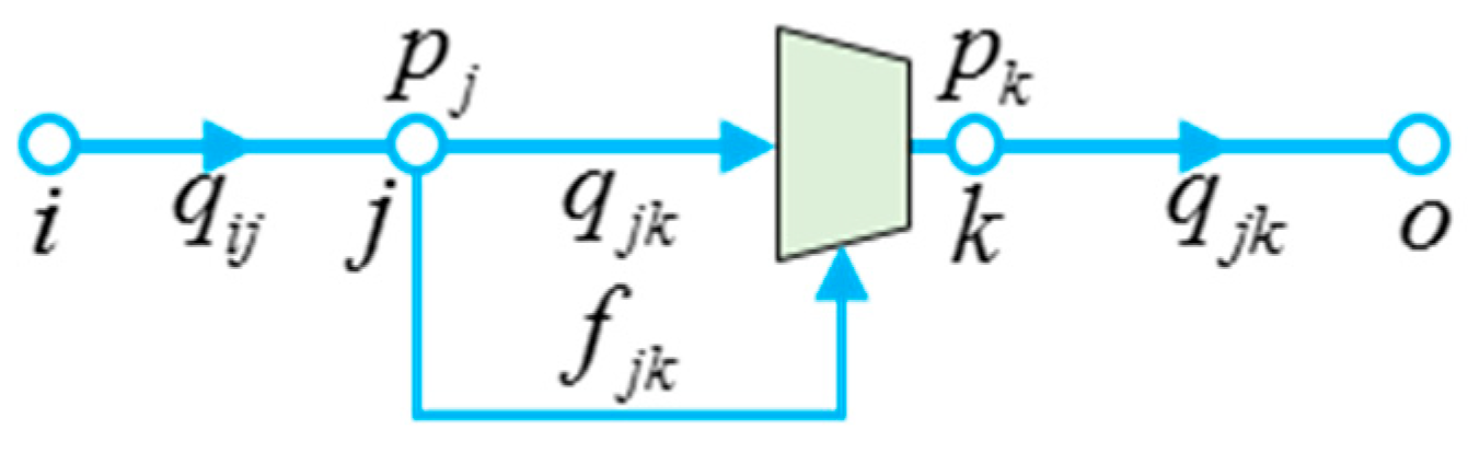
3.1.2. Natural Gas System

Natural gas system delivers energy to the load through natural gas pipelines, and its source is usually natural gas well or natural gas storage device, while the load is usually a variety of gas equipment [1,10]. The gas flow in pipeline is mainly controlled by adjusting the pressure of pressure regulating valves at different nodes. Next, it follows from [2,22,24] that, the steady state model of natural gas system is established.

For the ideal adiabatic natural gas pipeline, its start and end nodes are $i$ and $j$, respectively, and its steady state pipeline flow $q_{ij}$ is described by:

$$\{\begin{array}{c}{\pi }_{ij}{k}_{ij}{q}_{ij}^2=p_i^2-p_j^2\\ {\pi }_{ij}=\{\begin{array}{cc}+1& p_i\ge p_j\\ -1& p_i<p_j\end{array}\end{array}$$

(22)

where $p_i$ and $p_j$ represent the pressure of node $i$ and node $j$, respectively. $k_{ij}$ denotes a pipeline characteristic constant related to pipeline diameter, pipeline length, pipeline transmission efficiency, natural gas temperature, gas compression factor, etc., and the specific value can be found in [10,24,28]. ${\pi }_{ij}$ is the variable reflecting the direction of natural gas flow in the pipeline.

Due to the existence of friction resistance in the pipeline, transmission loss will be generated, which will lead to a certain pressure loss [16,29]. In order to ensure the reliability of long-distance energy transmission for natural gas pipeline network, a certain number of compressors should be installed in the natural gas system to compensate the pressure loss caused by friction.

Figure 2 shows schematic diagram of the pipeline with compressor driven by gas turbine. The mathematical model of natural gas pipeline with compressor can be expressed as follows:

$$\{\begin{array}{c}{f}_{jk}=k_{com}{q}_{jk}\left[{\left(r_{jk}\right)}^{\frac{\alpha -1}{\alpha }}-1\right]\\ q_{ij}=q_{jk}+f_{jk}\end{array}$$

(23)

where $f_{jk}$ denotes the natural gas flow consumed by the compressor. $k_{com}$ is the compressor characteristic constant. $q_{jk}$ denotes the natural gas flow through the compressor whose inlet node is $j$ and outlet node is $k$. $r_{jk}=p_k/p_j$ represents compression ratio of compressor. $\alpha$ denotes compressor variable index.

According to the law of flow conservation [22,30], the flow balance equation of each node in the natural gas network can be expressed in matrix form:

$${\mathbf{A}}_{\mathbf{c}}\dot{\mathbf{q}}+{\mathbf{A}}_{\mathbf{s}}\dot{\mathbf{f}}={\dot{\mathbf{q}}}_{\mathbf{0}}$$

(24)

where ${\mathbf{A}}_{\mathbf{c}}$ represents the node-branch complete incidence matrix of natural gas network. ${\mathbf{A}}_{\mathbf{s}}$ is the starting nodal association matrix of the natural gas network. $\dot{\mathbf{q}}$ denotes the flow vector of natural gas pipeline or branch. ${\dot{\mathbf{q}}}_{\mathbf{0}}$ represents the node net load flow vector in natural gas system. $\dot{\mathbf{f}}$ denotes the flow vector consumed by compressor in natural gas pipeline.

After developing the natural gas pipeline model and pipeline with compressor driven by gas turbine model, the directed graph is adopted to represent the topology structure of natural gas pipeline network based on the idea of graph theory, and the branch reference direction is set in advance. Assuming that the compressors are located at the first end of the pipeline and that the compressors do not affect the pipeline length, the matrix operation model of the natural gas system is formulated as:

$${\left({\mathbf{A}}_{\mathbf{s}}\mathbf{Diag}+{\mathbf{A}}_{\mathbf{e}}\right)}^{\prime }\dot{\mathbf{p}}={\dot{\mathbf{Q}}}_{\mathbf{q}}$$

(25)

where ${\mathbf{A}}_{\mathbf{e}}$ is the end nodal association matrix. $\dot{\mathbf{p}}={\left[p_1^2,p_2^2,\cdots ,p_{node}^2\right]}^{\prime }$ denotes the vector associated with the node pressure. ${\dot{\mathbf{Q}}}_{\mathbf{q}}={\left[{\pi }_1{k}_1{q}_1^2,{\pi }_2{k}_2{q}_2^2,\cdots ,{\pi }_b{k}_b{q}_b^2\right]}^{\prime }$ represents the vector associated with branch gas flow. $\mathbf{Diag}=diag\left(r_1^2,r_2^2,\cdots ,r_b^2\right)$ denotes the diagonal matrix for the compression ratio. The subscript $b$ is the branch or pipeline number. The subscript $node$ is the node number. ${(\cdot )}^{\prime }$ and ${[\cdot ]}^{\prime }$ denote the transpose of the matrix.

3.1.3. Heat System

Heat system is usually composed of heat source, heat network and heat load, which assume the functions of heat energy production, transmission and exchange. The heat network includes a supply water pipeline network and a return water pipeline network with water or steam as the heat transfer medium, which connects the heat source with the heat load [22]. Taking the supply water pipeline network as an example, the topology of heat network is described in this paper based on graph theory and the mature network topology description method in power system analysis [23,31]. The established heat system model is suitable for IES analysis, by combining the analysis method of hydraulic balance and thermal balance process in traditional thermal network.

Heat transfer medium flow in the network should meet the basic law of network: each nodal flow should meet the flow continuity equation [10,32,33]. In a closed loop of pipelines, the sum of the pressure head losses of heat transfer medium flow in each pipe is 0, which can be described by:

$$\{\begin{array}{c}{\mathbf{A}}_{\mathbf{h}}\dot{\mathbf{m}}={\dot{\mathbf{m}}}_{\mathbf{0}}\\ \mathbf{B}\left(\mathbf{\Delta }{\dot{\mathbf{H}}}_{\mathbf{b}}-{\dot{\mathbf{H}}}_{\mathbf{p}}\right)=\mathbf{0}\end{array}$$

(26)

where ${\mathbf{A}}_{\mathbf{h}}$ is the node-branch complete incidence matrix of heat system. $\mathbf{B}$ denotes the basic loop vector of heat system. $\dot{\mathbf{m}}$ denotes the pipeline or branch flow vector. ${\dot{\mathbf{m}}}_{\mathbf{0}}$ represents the net load flow of each node in heat system. $\mathbf{\Delta }{\dot{\mathbf{H}}}_{\mathbf{b}}$ is the pressure head losses vector of pipeline or branch in heat system, and the calculation method can be found in [10,28,33]. ${\dot{\mathbf{H}}}_{\mathbf{p}}$ represents the head vector of circulating pump in pipeline or branch in heat system.

The variables involved in the thermal model are nodal supply water temperature $T_s^{tem}$, nodal return water temperature $T_r^{tem}$ and nodal heat power [10,22], and heat power includes heat output $\Delta h_l$ of the heat source and heat demand $\Delta h_s$ of the load, which can be described by:

$$\{\begin{array}{l}\Delta h_l=C_p{m}_0^l\left(T_{s,l}^{tem}-T_{r,l}^{tem}\right)\\ \Delta h_s=C_p{m}_0^s\left(T_{s,s}^{tem}-T_{r,s}^{tem}\right)\end{array}$$

(27)

where $C_p$ is the specific heat capacity of heat transfer medium. $m_0^s$ and $m_0^l$ are the flow through the heat source and the heat load, respectively.

Considering the heat energy loss of the pipeline, the temperature drop of the heat transfer medium in its transmission is shown as:

$$T_{end,p}^{tem}-T_a^{tem}=\left(T_{start,p}^{tem}-T_a^{tem}\right)\exp \left(-\frac{{\lambda }_p{L}_p}{C_p{m}_p}\right)$$

(28)

where $T_{start,p}^{tem}$ and $T_{end,p}^{tem}$ are the heat transfer medium temperature at the starting point of the pipeline, and the heat transfer medium temperature at the ending point of the pipeline, respectively. $T_a^{tem}$ is the ambient temperature. $m_p$ denotes the flow rate of the pipeline, where the pipeline length is $L_p$ and the heat transfer coefficient is ${\lambda }_p$.

For any node in the heat network, the sum of the incoming thermal power is equal to the sum of the outgoing thermal power [3,10], so the temperature after convergence can be calculated by:

$$\left({\displaystyle \sum m_{out}}\right)T_{out}={\displaystyle \sum \left(m_{in}{T}_{in}\right)}$$

(29)

where $m_{out}$, and $T_{out}$ are the flow rate and temperature at the node outlet, respectively. $m_{in}$ and $T_{in}$ are the flow rate and temperature at the node entrance, respectively.

The heat network usually transmits heat energy to the heat load through the heat exchanger which is the equivalent heat load [33,34]. Another type of heat load is heating buildings, such as residential areas, huge shopping malls, large libraries, etc., which are here called ‘buildings’. This kind of heat load has strict requirements on temperature and needs to be modeled separately [21,25]. The following equivalent thermal parameter model can be employed to describe the characteristics of buildings, where the equation of state is discretized during programming:

$$\{\begin{array}{c}\underset{\dot{\mathbf{x}}}{\underbrace{\left[\begin{array}{c}{\dot{T}}_{in}\\ {\dot{T}}_{m,in}\end{array}\right]}}=\underset{\mathbf{A}}{\underbrace{\left[\begin{array}{cc}-\left(1/R_2{C}_a+1/R_1{C}_a\right)& 1/R_2{C}_a\\ 1/R_2{C}_m& -1/R_2{C}_m\end{array}\right]}}\underset{\mathbf{x}}{\underbrace{\left[\begin{array}{c}{T}_{in}\\ T_{m,in}\end{array}\right]}}+\underset{\mathbf{B}}{\underbrace{\left[\begin{array}{c}{T}_{out}/R_1{C}_a+H_l/C_a\\ 0\end{array}\right]}}\mathbf{u}\\ \mathbf{y}=\underset{\mathbf{C}}{\underbrace{\left[\begin{array}{cc}1& 0\\ 0& 1\end{array}\right]}}\underset{\mathbf{x}}{\underbrace{\left[\begin{array}{c}{T}_{in}\\ T_{m,in}\end{array}\right]}}+\underset{\mathbf{D}}{\underbrace{\left[\begin{array}{c}0\\ 0\end{array}\right]}}\mathbf{u}\end{array}$$

(30)

where $T_{in}$, $T_{m,in}$ and $T_{out}$ are indoor temperature, indoor air temperature, and outdoor environment temperature, respectively. $R_1$ and $R_2$ are the gain or heat loss coefficient. $C_a$ and $C_m$ are the heat capacity of air, and the mass heat capacity of buildings and their content, respectively. $H_l$ denotes the heating power of heating ventilation air conditioning system. $\mathbf{u}$ is the first order square matrix, and the element value is 1.

Remark 2.

Compared with [6,13,20], the developed IES model simultaneously coupling electric system, heat system and natural gas system can fully consider the key characteristic variables of each system, which really reflects “system level” operational characteristics. Furthermore, the matrix operation models about systems are also deduced firstly, as shown in (22)–(24), which can greatly facilitate the engineering calculation and application of large systems.

Remark 3.

On the basis of heat exchanger as heat load, an equivalent thermal parameter model of heat load is proposed, compared with the models developed in [10,23,31], the proposed model can better reflect the continuity and correlation of heat load in time, and it has more depth and accuracy to measure the characteristics of heat load by temperature, thus which can improve the flexible adjustment ability of heat load, and better reflects the heat load characteristic.

3.2. Multi-Objective Collaborative Optimization Model of Integrated Energy System

Through collaborative optimization of various energy and utilizing the coupling mechanism between multi-energy systems in time and space, IES reduces the utilization of fossil energy, and improves the utilization rate of renewable energy, thus reducing operating cost and improving the comprehensive utilization level of energy [26,30,35]. Therefore, an optimization model will be developed considering economic cost and renewable energy accommodation in the next part.

3.2.1. Economic Optimization Objective

As a complex energy system, IES has a variety of evaluation criteria. Under the background of current energy shortage, most analysis is based on reducing operating costs, in order to improve user economy. The specific optimization objective is given by:

$$\min f_1={\displaystyle \sum _{n=1}^N{\displaystyle \sum _{t=1}^T\left({\lambda }_{n,s,g}^t{F}_{n,s,g}^t+{\lambda }_{s,e}^t{P}_{s,e}^t\right)}}$$

(31)

where $F_{n,s,g}^t$ denotes the total amount of natural gas purchased by IES from natural gas source $n$ at time $t$, and the price of natural gas is ${\lambda }_{n,s,g}^t$. $P_{s,e}^t$ denotes the electricity purchased by IES from the large power grid at time $t$, and time-of-use electricity price (TOU) is expressed in ${\lambda }_{s,e}^t$.

3.2.2. Renewable Energy Accommodation Rate Optimization Objective

Improving the contribution of renewable energy and promoting the clean energy of using are also of vital importance to the rapid development of IES. Therefore, wind power absorption is taken as the optimization objective of IES. The objective function is given by:

$$\max f_2=\frac{{\displaystyle \sum _{t=1}^T\left(P_{wt}^{s,t}\right)}}{{\displaystyle \sum _{t=1}^T\left(P_{wt}^{s,a,t}\right)}}\cdot 100\%$$

(32)

where $P_{wt}^{s,a,t}$ and $P_{wt}^{s,t}$ denote the actual power injected into IES by WT, and the WT predicted output maximum power in the period $t$, respectively.

3.3. Optimization Constraints for Integrated Energy System

Power system constraints include tie line power exchange $P_{s,e}^t$ constraints, CHP unit active power $P_{CHP}^t$, reactive power $Q_{CHP}^t$ and heat power $H_{CHP}^t$ upper and lower bound constraints, node voltage $V_{node}^t$ upper and lower bound constraints and branch capacity $S_b^t$ constraints, which are formulated as:

$$\{\begin{array}{c}{P}_{s,e}^{\min }\le P_{s,e}^t\le P_{s,e}^{\max }\\ Q_{CHP}^{\min }\le Q_{CHP}^t\le Q_{CHP}^{\max }\\ {\alpha }_k{P}_{CHP}^t+{\beta }_k{H}_{CHP}^t\ge {\gamma }_k\\ V_{node}^{\min }\le V_{node}^t\le V_{node}^{\max }\\ S_b^{\min }\le S_b^t\le S_b^{\max }\end{array}$$

(33)

where ${\alpha }_k$, ${\beta }_k$ and ${\gamma }_k$ are the $k$th inequality constraint coefficients of CHP operating region.

Natural gas system constraints mainly include gas source injection power $F_{n,s,g}^t$ constraint, upper and lower limits of node pressure $p_i^t$, compressor compression ratio $r_b^t$ constraints, which can be summarized as:

$$\{\begin{array}{c}{F}_{n,s,g}^{\min }\le F_{n,s,g}^t\le F_{n,s,g}^{\max }\\ p_i^{\min }\le p_i^t\le p_i^{\max }\\ r_b^{\min }\le r_b^t\le r_b^{\max }\end{array}$$

(34)

In heating system, in order to ensure the high heating quality of the heat source and an efficient energy experience for terminal heat users, supply water temperature $T_{s,l}^{tem,t}$ of the heat source, return water temperature $T_{s,l}^{tem,t}$ of the heat load and flow rate $m_p^t$ in pipeline need to be limited. In addition, it is necessary to ensure that the node pressure head $h_b^t$ in heat network changes within the set range. The pressure head $h_p^t$ lifted by the circulation pump should be also limited to the maximum head range. It can be described by:

$$\{\begin{array}{c}{T}_{s,l}^{tem,\min }\le T_{s,l}^{tem,t}\le T_{s,l}^{tem,\max }\\ T_{s,l}^{tem,\min }\le T_{s,l}^{tem,t}\le T_{s,l}^{tem,\max }\\ m_p^{\min }\le m_p^t\le m_p^{\max }\\ h_b^{\min }\le h_b^t\le h_b^{\max }\\ h_p^{\min }\le h_p^t\le h_p^{\max }\end{array}$$

(35)

Terminal heat users or heat loads have a certain degree of fuzziness to the perception of comfortable temperature. In particular, for the buildings, in order to ensure the convenience of living, it is assumed that the flexible adjustment ability of buildings meets the following requirements: (1) Difference of indoor room actual temperature $T_{in}^{a,t}$ and the expected temperature $T_{in}^{\mathrm{e},t}$ is in a certain range [$-T_{in}^{\min }$,$T_{in}^{\max }$]. (2) The total actual temperature of indoor rooms ${\displaystyle \sum T_{in}^{a,t}}$ is equal to the total expected temperature of indoor rooms ${\displaystyle \sum T_{in}^{\mathrm{e},t}}$ within $T^{\prime }$ period. It is given as:

$$\{\begin{array}{c}-T_{in}^{\min }\le T_{in}^{a,t}-T_{in}^{\mathrm{e},t}\le T_{in}^{\max }\\ {\displaystyle \sum _{t=\tau }^{\tau =T^{\prime }}{T}_{in}^{a,t}}={\displaystyle \sum _{t=\tau }^{\tau =T^{\prime }}{T}_{in}^{\mathrm{e},t}}\end{array}$$

(36)

4. Solution Approach

The lower level multi-objective optimization model for EH and the upper level multi-objective optimization model for IES under off-design performance established above are typical 0–1 mixed integer non-linear optimization problems [10,30], which can be solved by using the method of 0–1 mixed integer non-linear programming (MINLP). In this paper, the solution approach to solve problems of lower and upper level, single and multi-objective optimization, and optimization process, can be clearly demonstrated and illustrated in Figure 3.

From Figure 3, optimization of each level includes single objective optimization and multi-objective optimization in this paper. Next, the related processes and concepts as shown in Figure 3 will be further explained.

4.1. Fuzzification of Objective Function

It is generally known that there are many methods to solve multi-objective optimization problem, and fuzzy optimization is one of the common methods. It is also universal to use fuzzy optimization to solve multi-objective optimization problems in academic papers, and this method is also employed in this paper.

Traditional fuzzy algorithm for solving multi-objective problems generally adopts increasing linear function or decreasing linear function as shown in Figure 4 (${\kappa }_n$ and ${\Delta }_n$ denote the characteristic parameter of increasing linear function and decreasing linear function). In this paper, the following continuous differentiable Sigmoid function or reverse Sigmoid function are used as membership function, the parameters of Sigmoid membership function are also determined. Because of applying improved membership functions, nonlinear programming methods are suitable to solve above multi-objective optimization model:

$$\mu (F_n)=\frac{1}{1+\exp \left[-{\omega }_1\left(F_n-{\omega }_2\right)\right]}$$

(37)

$$\mu (F_n)=1-\frac{1}{1+\exp \left[-{\omega }_1\left(F_n-{\omega }_2\right)\right]}$$

(38)

where ${\omega }_1$ and ${\omega }_2$ denote characteristic parameter of Sigmoid and reverse Sigmoid function.

The Sigmoid function curve has the same semi-open shape as increasing linear function curve, so it is suitable for the membership function described as the “maximum” issue. In order to make the shape of Sigmoid function as close as possible to the original increasing linear function, in particular, to keep the coincidence of the points (waist values) of the two curves at $\mu (F_n)=0.5$, the points at $\mu (F_n)=0.5$ and 0.9 (shoulder value) in this paper are taken as coincident points, which can be used to obtain the Sigmoid characteristic parameters, and vice versa.

The optimization problem with fuzzy objective function and constraint condition or one of them is called fuzzy optimization problem. When there is more than one objective, it is then called multi-objective fuzzy optimization problem. According to the maximum minimum satisfaction degree method, the satisfaction degree $\mathsf{ƛ}$ is the minimum value in the membership function of all objective functions, that is, $\mathsf{ƛ}=\min \left\{\mu (F_n)\right\}$. According to the maximum and minimum principle of fuzzy set theory, the multi-objective optimization problem can be transformed into the problem of $\mathsf{ƛ}$ maximization with meeting all constraints, that is, the $\max \mathsf{ƛ}$ problem, which is described by:

$$\begin{array}{l}\max \mathsf{ƛ}\\ s.t.\{\begin{array}{c}\mu (F_n)\ge \mathsf{ƛ}\\ 0\le \mathsf{ƛ}\le 1\\ \left(1\right)–\left(38\right)\end{array}\end{array}$$

(39)

Remark 4.

Based on fuzzy theory, a multi-objective fuzzy collaborative optimization model for EH and IES is developed, the continuous differentiable Sigmoid function is introduced as an improved membership function. Therefore, the nonlinear programming methods are better reasonable and suitable to solve above multi-objective optimization model for applying the improved membership functions.

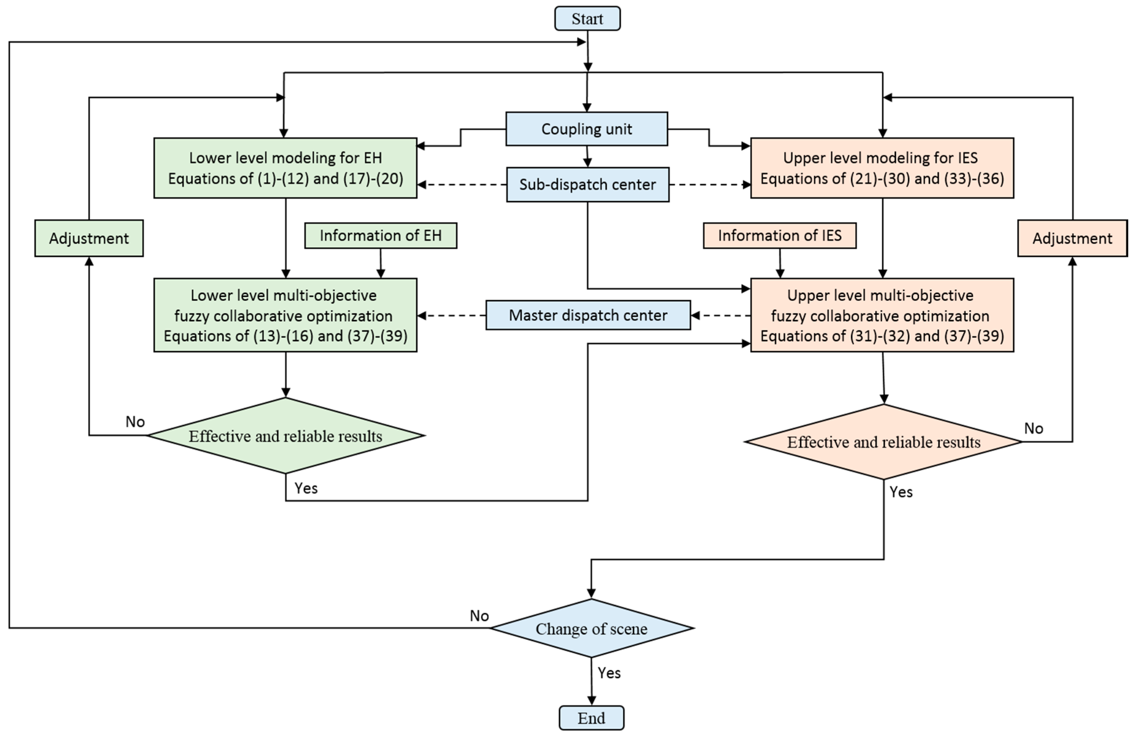
4.2. Optimization Framework

The framework of hierarchical multi-objective fuzzy collaborative optimization method is provided in Figure 5. From Figure 5, the high-order nonlinear models of devices under off-design performance and optimization models are presented in lower level for EH, which can be represented by Equations (1)–(20) and (37)–(39). And subsystem “energy system” models and optimization models are proposed in upper level for IES, which can be represented by Equations (21)–(39). Based on the relationship between master and slave dispatching center, Firstly, the lower level model about EH is optimized including single objective optimization and multi-objective optimization, where the various detailed data are obtained from the lower level optimization results. Secondly, facing different engineering application modes, the lower level dispatching center uploads the data of the lower level optimization results to the upper level dispatching center, which prepare for upper level optimization. Then, the upper level optimization also includes single objective optimization and multi-objective optimization, after optimizing the upper level model about IES, and the upper level dispatching center feeds back the updated scheduling plan to the lower level dispatching center. This “hierarchical collaborative optimization” strategy can well adapt to and reflect real world energy system where engineering application modes are diversified.

In view of the hierarchical multi-objective fuzzy collaborative optimization model developed in this paper, where it’s essentially MINLP, general commercial optimization software, such as LINGO, GAMS, CPLEX and so on, can be used to solve it. Programs are written based on the LINGO18.0 optimization software platform (LINDO & LINGO (TIANJIN) TECH. CO., LTD, TIANJIN, CHINA) and the global solver is utilized to solve the above problems.

5. Case Study

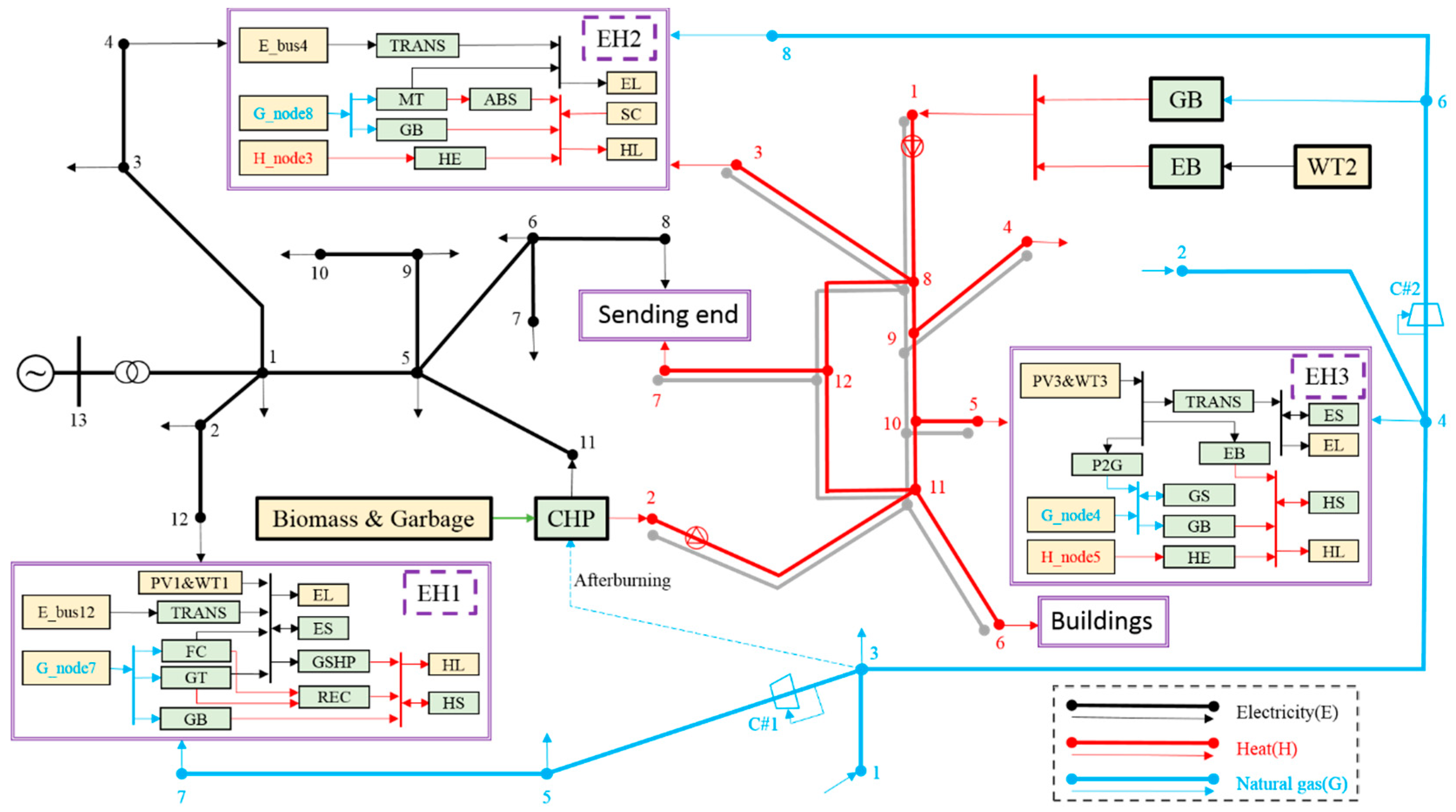
5.1. System Description

The typical days in winter are taken as the research object, which is divided into 24 periods (that is, an optimal dispatch cycle). The specific structure of the model is shown in Figure 6.

IES consists mainly of 13 power system nodes, eight natural gas system nodes, 12 heat system nodes and three EHs (recorded as EH1, EH2 and EH3, respectively). The three systems are directly coupled together through CHP unit, in which the fuel required by CHP is mainly provided by biomass and garbage, and the natural gas imported to CHP unit plays a role of afterburning. Natural gas system and heat system are directly coupled through GB. To take full advantage of the geographical resource endowment, wind farm (WT3) provides heat energy to heat system through EB during the day. In order to ensure safe and reliable power supply of power system, the power system interconnects with the large power grid through node 13. Natural gas system mainly relies on node 1 gas source and node 2 gas source to obtain natural gas. Three systems are indirectly coupled with EH1, EH2 and EH3, and the electricity, heat and gas input into EH work together. Three EH in lower layer and three systems in the upper layer all work together to maximize the comprehensive benefit.

The maximum startup times of FC, GT, GB, GSHP, MT, and so on in a scheduling cycle are all 4. The parameter settings of each device under off-design performance are all from the corresponding references. All the factors of equations (1)–(7) are reported in

Table A1. Factors parameters of main devices.

Types	Value
$a_0\sim a_5$	[17]
$b_0\sim b_4$	[17]
$c_0\sim c_3$	0.0926, 0.8365, −1.0135, 0.4166
$d_0\sim d_3$	0.82869, 0.30173, 0.24644, 0.16371
$e_0\sim e_2$	0.0951, 1.5250, 0.6249
$f_0\sim f_2$	[18]
$g_0\sim g_2$	[18]
$h_0\sim h_3$	4.08 × 10−4, 0.107, −8.910 × 10−5, 0.169
$j_0\sim j_3$	1.9550, -2.3635, 1.9146, −0.5061
$k_0\sim k_2$	0.0488, 0.8184, 0.1328
$m_0\sim m_5$	−0.0558, 0.0280, −0.4724, 1.7780, −0.5555, 0.2777

of Appendix A, and IES subsystem topology information are showed in

Table A2. Topology information of the IES case.

Power System	Branch	From node	To node
	1	13	1
	2	1	2
	3	1	5
	4	1	3
	5	5	6
	6	5	11
	7	5	9
	8	2	12
	9	3	4
	10	6	7
	11	6	8
	12	9	10
Heat System	Pipeline	From node	To node
	1	1	8
	2	2	11
	3	8	3
	4	9	4
	5	10	5
	6	11	6
	7	12	7
	8	8	9
	9	10	9
	10	11	10
	11	11	12
	12	8	12
Natural Gas System	Pipeline	From node	To node
	1	1	3
	2	2	4
	3	4	3
	4	5	7
	5	6	8
	6	3	5
	7	4	6

of Appendix B. GSHP is allowed to work during periods from 7 to 24. TRAN’s efficiency and TOU references [10,12,23]. The units of power in this paper are MW unless otherwise specified. The objectives selected for EH1 are $F_1$, $F_2$ and $F_3$. For EH2, $F_1$ and $F_4$ are selected as its objectives. For EH3, $F_1$ and $F_4$ are selected for its objectives. $f_1$ and $f_2$ are selected as IES’s objectives.

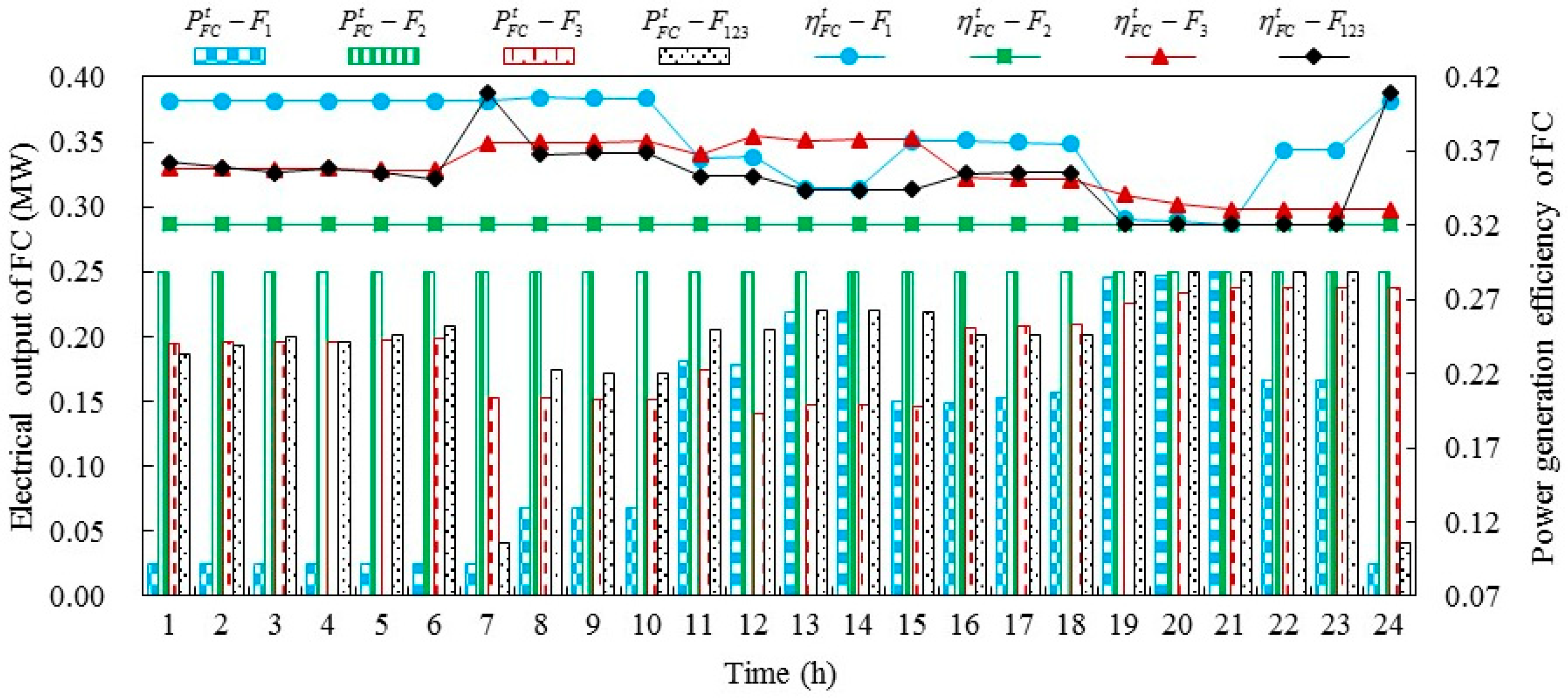
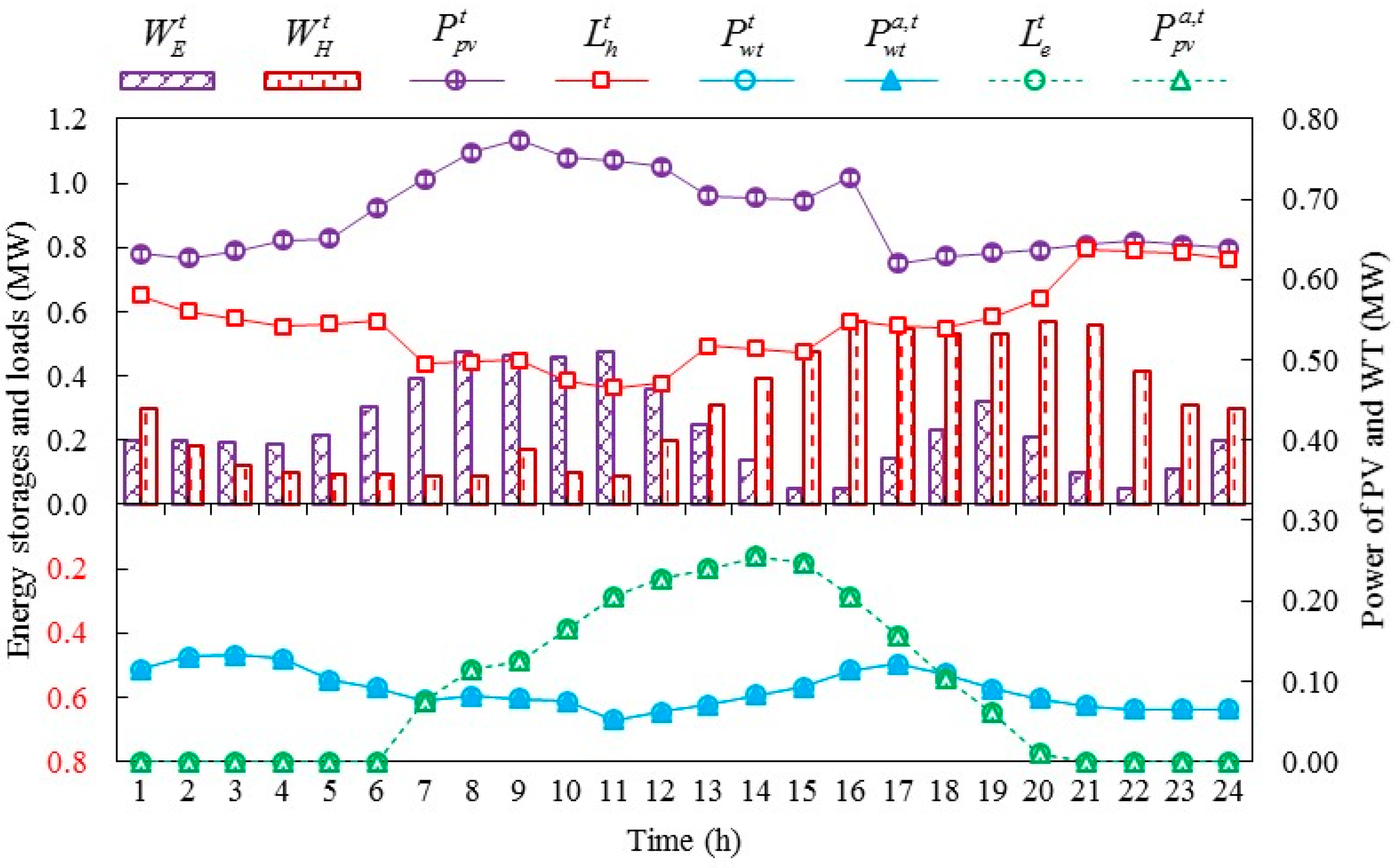
5.2. Results and Analyses

The results of single objective and multi-objective fuzzy optimization are shown in

Table 1. Single-objective and multi-objective fuzzy collaborative optimization results.

EH1	Single Objective	Optimal Results of Single Objective				Optimal Results of Multi-Objective Fuzzy Optimization
		Result of${\mathit{F}}_{\mathbf{1}}$	Result of${\mathit{F}}_{\mathbf{2}}$		Result of${\mathit{F}}_{\mathbf{3}}$
	$F_1$/CNY	15,200.79	15.25		56.31	15,784.01
	$F_2$/t	17,183.68	13.09		54.39	13.72
	$F_3$/MW	16,468.89	13.54		52.97	53.86
EH2	Single Objective	Optimal Results of Single Objective				Optimal Results of Multi-Objective Fuzzy Optimization
		Result of ${\mathit{F}}_{\mathbf{1}}$		Result of ${\mathit{F}}_{\mathbf{4}}$
	$F_1$/CNY	12,979.03		59.31		13,878.65
	$F_4$/%	14,642.73		100.00		78.58
EH3	Single Objective	Optimal Results of Single Objective				Optimal Results of Multi-Objective Fuzzy Optimization
		Result of ${\mathit{F}}_{\mathbf{1}}$		Result of ${\mathit{F}}_{\mathbf{4}}$
	$F_1$/CNY	3568.04		96.79		4341.03
	$F_4$/%	5769.80		97.26		97.03
IES	Single Objective	Optimal Results of Single Objective				Optimal Results of Multi-Objective Fuzzy Optimization
		Result of ${\mathit{f}}_{\mathbf{1}}$		Result of ${\mathit{f}}_{\mathbf{2}}$
	$f_1$/CNY	67,473.95		80.75		67,004.26
	$f_2$/%	66,286.33		92.31		87.16

.

Taking EH3 as an example, satisfaction degree $\mathsf{ƛ}$ of multi-objective fuzzy optimization is 0.705874. At this time, operating fuel cost of multi-objective fuzzy optimization increases by 3.84% compared with $F_1$, pollutant gas emission increases by 4.85% compared with $F_2$, and primary fossil energy consumed increases by 1.6% compared with $F_3$. Multi-objective fuzzy optimization balances the contradictions and conflicts among each single objective, and takes into account the comprehensive requirements of each objective, and obtains an optimal scheduling scheme which is satisfactory to all parties. Multi-objective fuzzy optimization can more accurately reflect the actual operation of EHs and IES, and has obvious advantages over single objective optimal scheduling model.

In this paper, only FC is taken as an example to analyze the variation of device energy efficiency under off-design performance and the difference of device operation mode under different optimization objectives. As shown in Figure 7, when the generation power of FC is high, its power generation efficiency will be reduced accordingly. During the time period from 1 to 10, the power generation efficiency of FC under different optimization objectives is relatively stable, but there is a significant difference between power generation efficiency under $F_1$ and $F_2$, and the cost of operating fuel under $F_1$ is the least and the fuel can be saved under the running mode of high generation efficiency. However, the minimum emission is sought under $F_2$, and the $C{O}_2$ emission factor of FC is obviously smaller than that of GT. It is obvious that the full power operation of FC under $F_2$ is much helpful to reduce emissions.

Under the multi-objective fuzzy collaborative optimization mode, change of energy level including electrical and heat energy storage equipment and renewable energy accommodation for EH1 during each period are shown in Figure 8. Results from Figure 8 show that renewable energy is completely absorbed, although multi-objective optimization of EH1 does not take into account the optimal problem about renewable energy accommodation. Increasing the penetration of renewable energy by EH1 can reduce the cost of purchasing electricity and natural gas while EH1 runs under the actual optimized scheduling and reduce fossil fuel combustion emissions, at the same time, increasing the given renewable energy can be equivalent to reduce the consumption of fossil fuels. As shown in Figure 8, the time periods from 1 to 9 are the periods of valley-flat electricity price, and ES is always in the charging state. The periods from 10 to16 are the periods of flat-peak electricity price, ES is always in the state of discharge. PV power can be fully absorbed during time periods from 17 to 19. ES can effectively reduce operating costs, pollution emissions and fossil energy consumption in optimal scheduling cycle. HS is mainly in the state of heat storage from time period 10 to time period 17, at the same time, and this period is the low period of heat load. It is in the exothermic state during the time periods from 21 to 6, where this period is the peak and valley period of heat load. It can be seen that HS can effectively deflate and bridge the peak and valley difference of heat load. Energy flows mode of EH are optimized by the coordination of various energies and equipment, which highlights the benefits of coordinated optimal operation.

In EH2, GB is the direct coupling device of natural gas and heat energy, while MT is the direct key coupling device of electricity, heat and natural gas. GB and MT work together, in which the amount of natural gas entering MT from natural gas node 8 can be reflected by the allocation proportion factor ($v_{MT}^t$). Figure 9 shows change of power generation efficiency and allocation proportion factor of MT, and power of SC for EH2 under different optimization objectives in different time periods. As can be seen from Figure 9, as long as MT works, no matter in which optimization mode, $v_{MT}^t$’s value is greater than 0.8, which indicates that, compared with GB, MT’s operation plays a major role in consuming natural gas, while GB actually plays a role in afterburning. In addition, $v_{MT}^t$ of MT is relatively stable under $F_1$, that is, natural gas node 8 supply of natural gas will be relatively stable. In general, power generation efficiency of MT is relatively stable under different optimization scenarios, all of which are around 0.38. The stable power generation efficiency of MT is also good for ABS stabilization work, which is beneficial to the coordination of MT and ABS. Figure 9 shows that under different optimization modes, the actual output of SC is significantly different. There are no energy storages equipment in EH2, compared with EH1, and it is clear that there is no free and flexible absorption of solar energy. But under $F_4$, the actual power accepted output of SC has reached 78.58%, which is relatively acceptable in actual operation, and multi-objective fuzzy optimization has achieved the desired results.

Node 1 in the natural gas system is the pressure reference point, which is also the gas source point. The results of Figure 10 show that the pressure values of each node are (0.8p.u., 1.2p.u.) in the whole IES optimal scheduling cycle as opposed to the pressure of the reference point, which fully meet the pressure setting requirements. The nodal pressure of the compressor downstream is mainly adjusted by the compressor to maintain its safety and reasonable range. The nodal pressure of compressor upstream is mainly regulated by natural gas source 2, that is, node 2. From Figure 10, it can be found that the pressure fluctuation of node 2 is relatively large, and the natural gas source 2 plays a role in balancing the pressure stability of the whole natural gas system’s node to a certain extent.

Figure 11 shows that the actual temperature in the room well tracks the expected temperature well during IES optimization scheduling cycle, which indicates that the thermal parameter equivalent model developed for buildings is effective. The change of the actual temperature in the room not only meets the requirements of thermal users, but also increases the flexibility of IES scheduling and endows heat load with certain flexible characteristics.

In Figure 6, the heat system is a central heating system with double heat sources, multiple heat load types and loops. The loop can guarantee the reliability of heating, and some pipelines on the loop are often in a standby state in practical operation. From Figure 12, it can be found that heat source #1 mainly provides heat energy to nearby heat load #3 and heat load #4, while heat source #2 provides heat energy to nearby heat load #5, heat load #6 and heat load #7. This kind of nearby heating characteristic of heat source is very common under the practical engineering application, which gives priority to nearby heating, avoids the long distance transmission heat transfer medium flow, and reduces the heat energy loss.

6. Conclusions

According to the requirements of practical engineering applications in real world situation, this paper proposed a hierarchical multi-objective fuzzy collaborative optimization model for IES under off-design performance. Lower level multi-objective fuzzy collaborative optimization model mainly centered on EH, where models of various devices under off-design performance were established in detail. Lower level model is mainly oriented to regional or industrial park IES, which can adapt to the optimization and regulation analysis of IES in the real world. Upper level multi-objective fuzzy collaborative optimization model of IES including power system, natural gas system, and heat system was proposed based on the relationship between master and slave dispatch centers. Upper level model has large potential and wide applications in analyzing optimal operation of regional multi-energy coupling systems in the real world.

The models were applied and verified by a chosen case study of IES, where the case and optimization model in this paper can well adapt to and reflect real world energy system. The results demonstrated the availability of regarding the proposed multi-objective fuzzy collaborative optimization under off-design performance conditions as the basis of performance analysis of devices, calculation and operation analysis of EH, optimal scheduling, collaborative operation of hybrid multi-energy system, the planning of different operation modes, and engineering calculation analysis of IES.

References

1. Zeng, Q.; Zhang, B.; Fang, J.; Chen, Z. Coordinated operation of the electricity and natural gas systems with bi-directional energy conversion. Energy Procedia 2017, 105, 492–497. [Google Scholar] [CrossRef]
2. Yang, L.; Zhao, X.; Li, X.; Yan, W. Probabilistic steady-state operation and interaction analysis of integrated electricity, gas and heating systems. Energies 2018, 11, 917. [Google Scholar] [CrossRef]
3. Liu, X.; Jenkins, N.; Wu, J.; Bagdanavicius, A. Combined analysis of electricity and heat networks. Energy Procedia 2014, 61, 155–159. [Google Scholar] [CrossRef]
4. Habibollahzade, A.; Gholamian, E.; Behzadi, B. Multi-objective optimization and comparative performance analysis of hybrid biomass-based solid oxide fuel cell/solid oxide electrolyzer cell/gas turbine using different gasification agents. Appl. Energy 2019, 233, 985–1002. [Google Scholar] [CrossRef]
5. Dong, S.; Wang, C.; Xu, S. Day-ahead optimal scheduling of electricity-gas-heat integrated energy system considering dynamic characteristics of networks. Autom. Electr. Power Syst. 2018, 42, 12–19. [Google Scholar]
6. Hao, R.; Ai, Q.; Zhu, Y. Hierarchical optimal dispatch based on energy hub for regional integrated energy system. Electr. Power Autom. Equip. 2018, 37, 171–178. [Google Scholar]
7. Bai, L.; Li, F.; Cui, H.; Jiang, T.; Sun, H.; Zhu, J. Interval optimization based operating strategy for gas-electricity integrated energy systems considering demand response and wind uncertainty. Appl. Energy 2016, 167, 270–279. [Google Scholar] [CrossRef] [Green Version]
8. Ha, T.; Zhang, Y.; Hao, J.; Thang, V.; Li, C. Energy hub’s structural and operational optimization for minimal energy usage costs in energy systems. Energies 2018, 11, 707. [Google Scholar] [CrossRef]
9. Geidl, M.; Andersson, G. Optimal power flow of multiple energy carriers. IEEE Trans. Power Syst. 2007, 22, 145–155. [Google Scholar] [CrossRef]
10. Zhong, Y.; Xie, D.; Zhai, S.; Sun, Y. Day-ahead hierarchical steady state optimal operation for integrated energy system based on energy hub. Energies 2018, 11, 2765. [Google Scholar] [CrossRef]
11. Wei, D.; Chen, A.; Sun, B. Multi-objective optimal operation and energy coupling analysis of combined cooling and heating system. Energy 2016, 98, 296–307. [Google Scholar] [CrossRef]
12. Ma, T.; Wu, J.; Hao, L. Energy flow modeling and optimal operation analysis of micro energy grid based on energy hub. Power Syst. Technol. 2018, 133, 292–306. [Google Scholar] [CrossRef]
13. Ma, H.; Wang, B.; Gao, W.; Liu, D. Optimal scheduling of an regional integrated energy system with energy storage systems for service regulation. Energies 2018, 11, 195. [Google Scholar] [CrossRef]
14. Xu, J.; Shi, J.; Zhang, J. Bi-level optimization of urban integrated energy system based on biomass combined heat and power supply. Autom. Electr. Power Syst. 2018, 42, 23–31. [Google Scholar]
15. Ayele, G.; Haurant, P.; Laumert, B.; Lacarrière, B. An extended energy hub approach for load flow analysis of highly coupled district energy networks: Illustration with electricity and heating. Appl. Energy 2018, 212, 850–867. [Google Scholar] [CrossRef]
16. Zhou, X.; Guo, C.; Wang, Y.; Li, W. Optimal expansion co-planning of reconfigurable electricity and natural gas distribution systems incorporating energy hubs. Energies 2017, 10, 124. [Google Scholar] [CrossRef]
17. El-Sharkh, M.; Rahman, A.; Alam, M. Thermal energy management of a CHP hybrid of wind and a grid-parallel PEM fuel cell power plant. In Proceedings of the 2009 IEEE Power and Energy Society General Meeting, Calgary, AB, Canada, 26–30 July 2009. [Google Scholar]
18. Li, J.; Tian, L.; Cheng, L. Optimal planning of micro-energy system considering off-design performance part one general model and analysis. Autom. Electr. Power Syst. 2018, 42, 18–26. [Google Scholar]
19. Cui, Y.; Yang, Z.; Zhong, W. A joint scheduling strategy of CHP with thermal energy storage and wind power to reduce sulfur and nitrate emission. Power Syst. Technol. 2018, 42, 1064–1071. [Google Scholar]
20. Li, F.; Sun, B.; Zhang, C.; Zhang, L. Operation optimization for combined cooling, heating, and power system with condensation heat recovery. Appl. Energy 2018, 230, 305–316. [Google Scholar] [CrossRef]
21. Li, H.; Kang, S.; Yu, Z. A feasible system integrating combined heating and power system with ground-source heat pump. Energy 2014, 74, 240–247. [Google Scholar] [CrossRef]
22. Linna, N.; Liu, W.; Wen, F. Optimal operation of electricity, natural gas and heat systems considering integrated demand responses and diversified storage devices. J. Modern Power Syst. Clean Energy 2018, 6, 423–437. [Google Scholar]
23. Lu, Z.; Yang, Y.; Geng, L. Low-carbon economic dispatch of the integrated electrical and heating systems based on benders decomposition. Proc. CSEE 2018, 38, 1922–1934. [Google Scholar]
24. Li, G.; Zhang, R.; Jiang, T. Security-constrained bi-level economic dispatch model for integrated natural gas and electricity systems considering wind power and power-to-gas process. Appl. Energy 2017, 194, 696–704. [Google Scholar] [CrossRef]
25. Wang, Y.; Yu, H.; Yong, M.; Huang, Y.; Zhang, F.; Wang, X. Optimal scheduling of integrated energy systems with combined heat and power generation, photovoltaic and energy storage considering battery lifetime loss. Energies 2018, 11, 1676. [Google Scholar] [CrossRef]
26. Martinezmares, A.; Fuerteesquivel, C. A robust optimization approach for the interdependency analysis of integrated energy systems considering wind power uncertainty. IEEE Trans. Power Syst. 2013, 28, 3964–3976. [Google Scholar] [CrossRef]
27. Huang, Y.; Yang, K.; Zhang, W.; Lee, K. Hierarchical energy management for the multienergy carriers system with different interest bodies. Energies 2018, 11, 2834. [Google Scholar] [CrossRef]
28. Liu, X.; Mancarella, P. Modelling, assessment and sankey diagrams of integrated electricity-heat-gas networks in multi-vector district energy systems. Appl. Energy 2016, 167, 336–352. [Google Scholar] [CrossRef]
29. Wu, L.; Wu, Q.; Jing, Z. Optimal power and gas dispatch of the integrated electricity and natural gas networks. In Proceedings of the 2016 IEEE Innovative Smart Grid Technologies–Asia, Melbourne, Australia, 28 November–1 December 2016. [Google Scholar]
30. Wang, D.; Liu, L.; Jia, H.; Wang, W. Review of key problems related to integrated energy distribution systems. CSEE J. Power Energy Syst. 2018, 4, 130–145. [Google Scholar] [CrossRef]
31. Aghtaie, M.; Dehghanian, P.; Firuzabad, M.; Abbaspour, A. Multiagent genetic algorithm: An online probabilistic view on economic dispatch of energy hubs constrained by wind availability. IEEE Trans. Sustain. Energy 2013, 1, 699–708. [Google Scholar]
32. Li, J.; Niu, D.; Wu, M.; Wang, Y.; Li, F.; Dong, H. Research on battery energy storage as backup power in the operation optimization of a regional integrated energy system. Energies 2018, 11, 2990. [Google Scholar] [CrossRef]
33. Gou, X.; Chen, Q.; Hu, K.; Ma, H.; Chen, L.; Wang, X.; Qi, J.; Xu, F.; Min, Y. Optimal planning of capacities and distribution of electric heater and heat storage for reduction of wind power curtailment in power systems. Energy 2018, 160, 763–773. [Google Scholar] [CrossRef]
34. Clegg, S.; Mancarella, P. Integrated electricity-heat-gas modelling and assessment, with applications to the Great Britain system. Part I: High-resolution spatial and temporal heat demand modelling. Energy 2018. [Google Scholar] [CrossRef]
35. Ahmadi, P.; Dincer, I.; Rosen, M. Thermoeconomic multi-objective optimization of a novel biomass-based integrated energy system. Energy 2014, 68, 958–970. [Google Scholar] [CrossRef]
Figure 1. A typical FC case under off-design performance: (a) Schematic diagram of FC working principle; (b) Off-design performance of FC.
Energies 12 00830 g001
Figure 2. Pipeline with compressor driven by gas turbine.
Energies 12 00830 g002
Figure 3. Hierarchical optimization process.
Energies 12 00830 g003
Figure 4. Fuzzy membership function: (a) Increasing linear function and Sigmoid function; (b) Decreasing linear function and reverse Sigmoid function.
Energies 12 00830 g004
Figure 5. Framework of proposed fuzzy collaborative optimization method for IES.
Energies 12 00830 g005
Figure 6. Schematic diagram of the integrated energy system.
Energies 12 00830 g006
Figure 7. Change of power generation efficiency and electrical output for FC under different optimization objectives in different time periods.
Energies 12 00830 g007
Figure 8. Change of energy storages and renewable energy accommodation for EH1 under multi-objective fuzzy optimization mode in different time periods.
Energies 12 00830 g008
Figure 9. Change of power generation efficiency and allocation proportion factor of MT, and power of SC for EH2 under different optimization objectives in different time periods.
Energies 12 00830 g009
Figure 10. Change of nodal pressure in natural gas system under f 12 .
Energies 12 00830 g010
Figure 11. Indoor temperature changes of buildings under f 12 .
Energies 12 00830 g011
Figure 12. Changes in the mass flow rate of the pipelines connecting sources and loads under f 12 .
Energies 12 00830 g012