Wenner Soundings for Apparent Resistivity Measurements at Small Depths Using a Set of Unequal Bare Electrodes: Selected Case Studies


Abstract
:1. Introduction
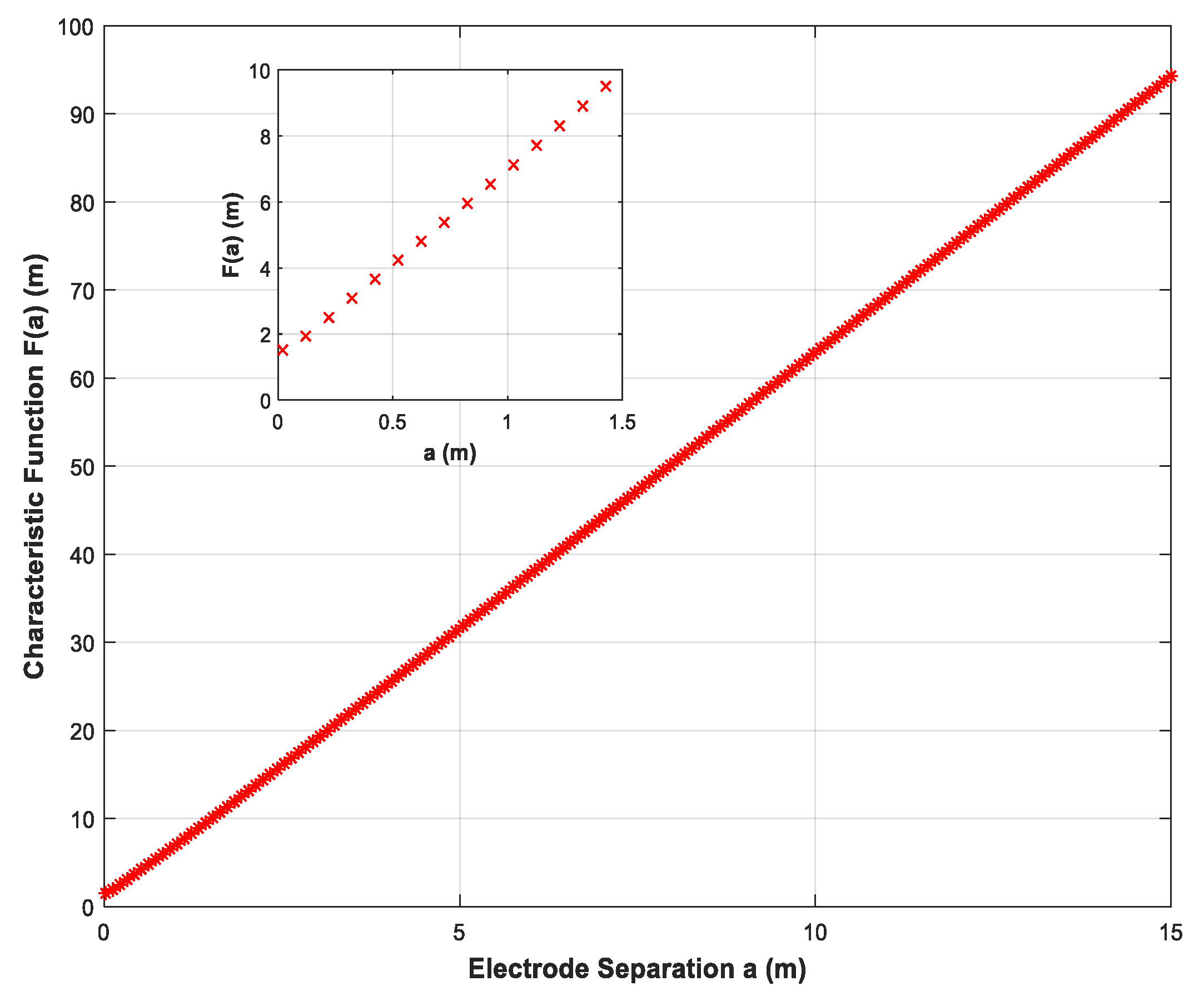
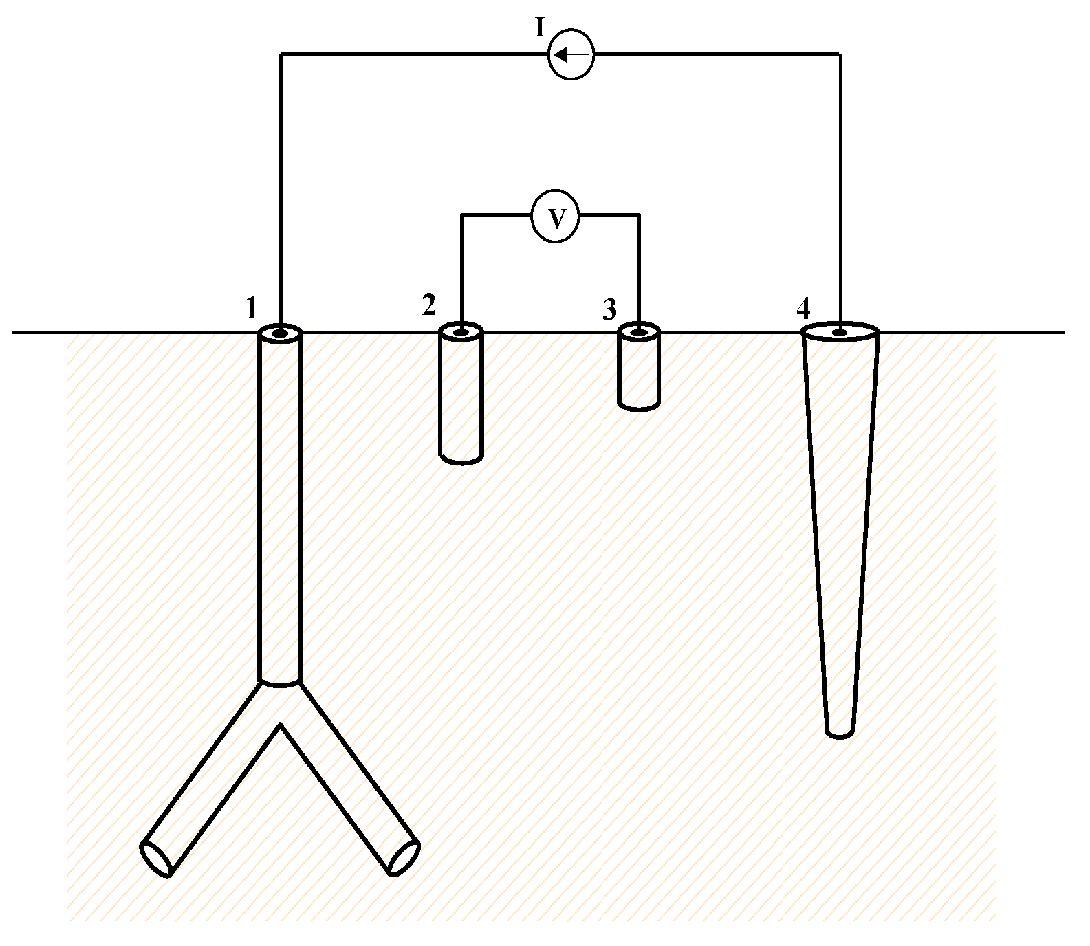
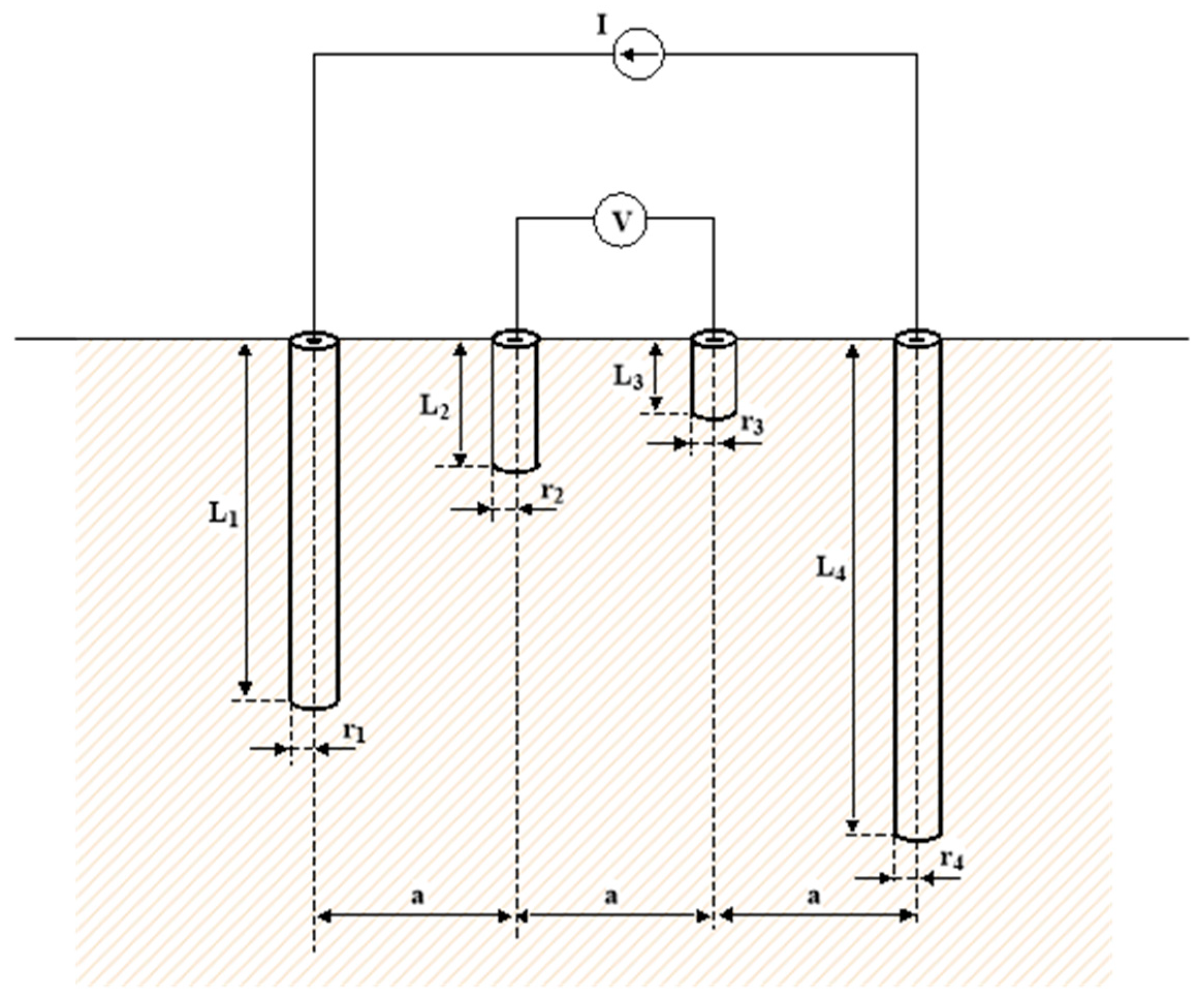
2. Theoretical Background
3. Application to Selected Case Studies
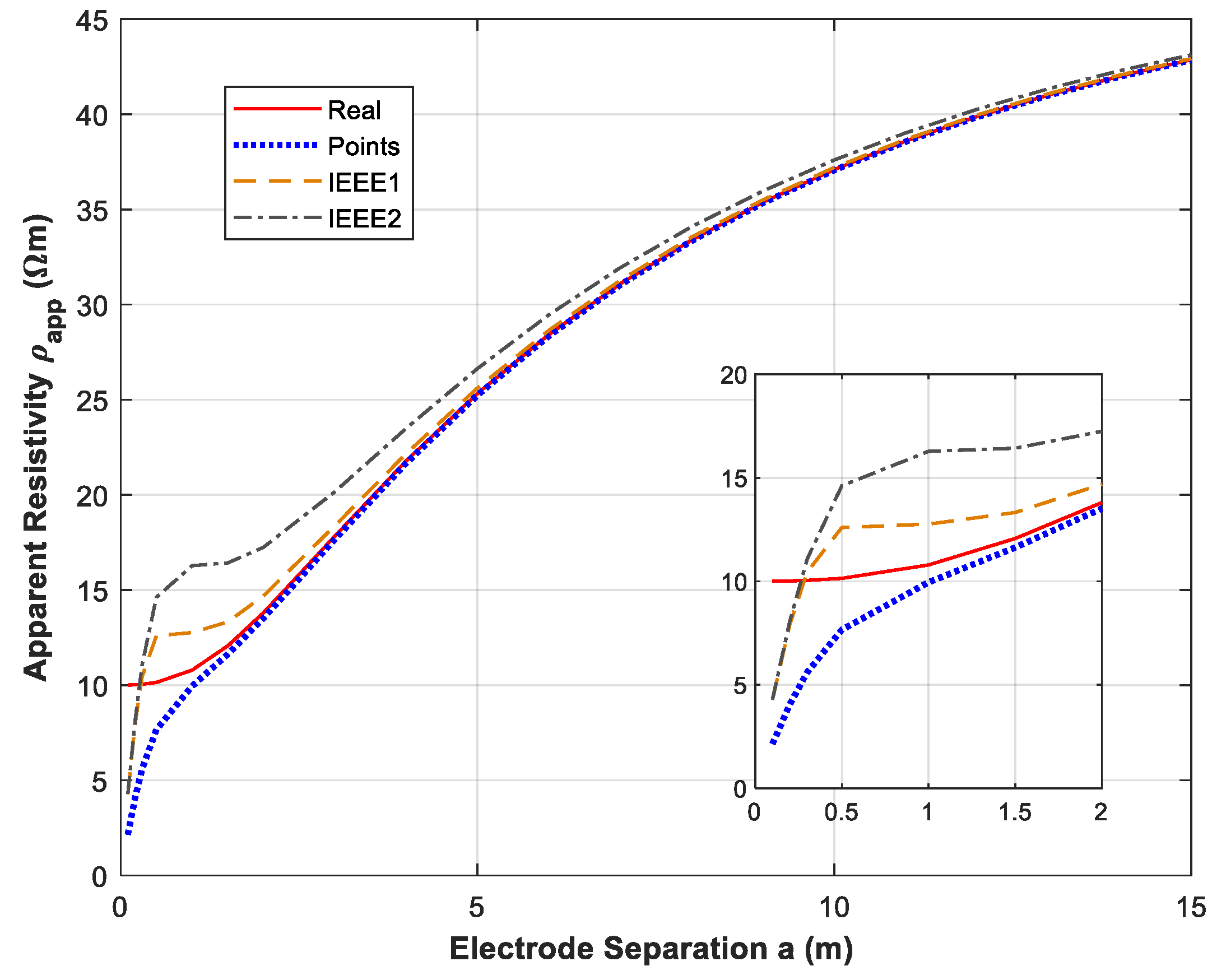
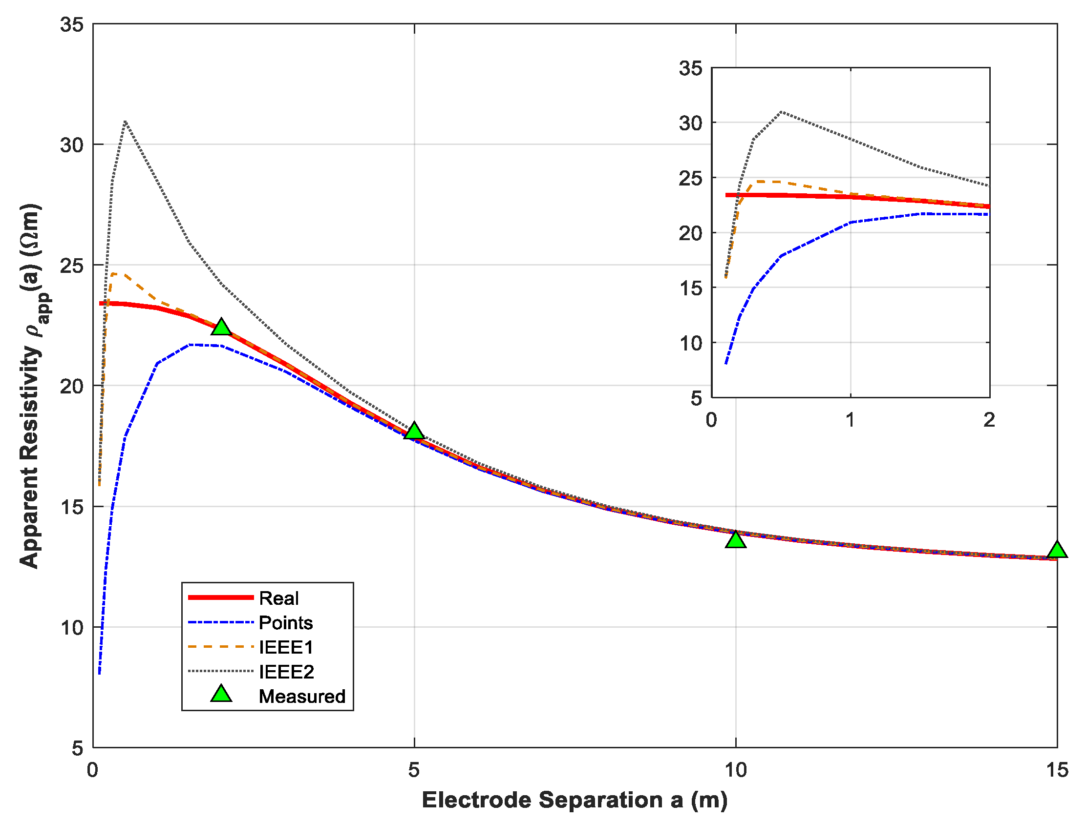
3.1. Case Study 1
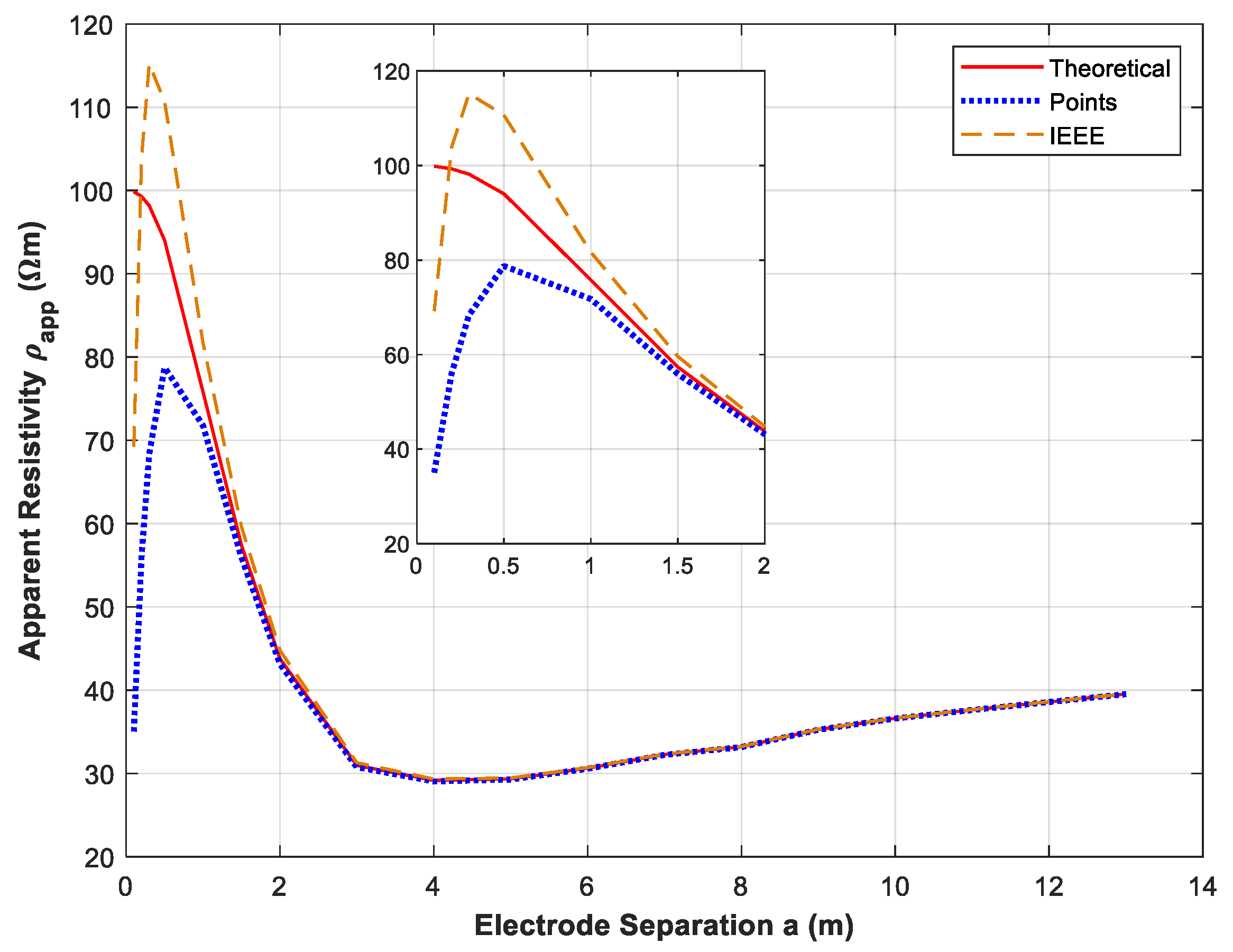
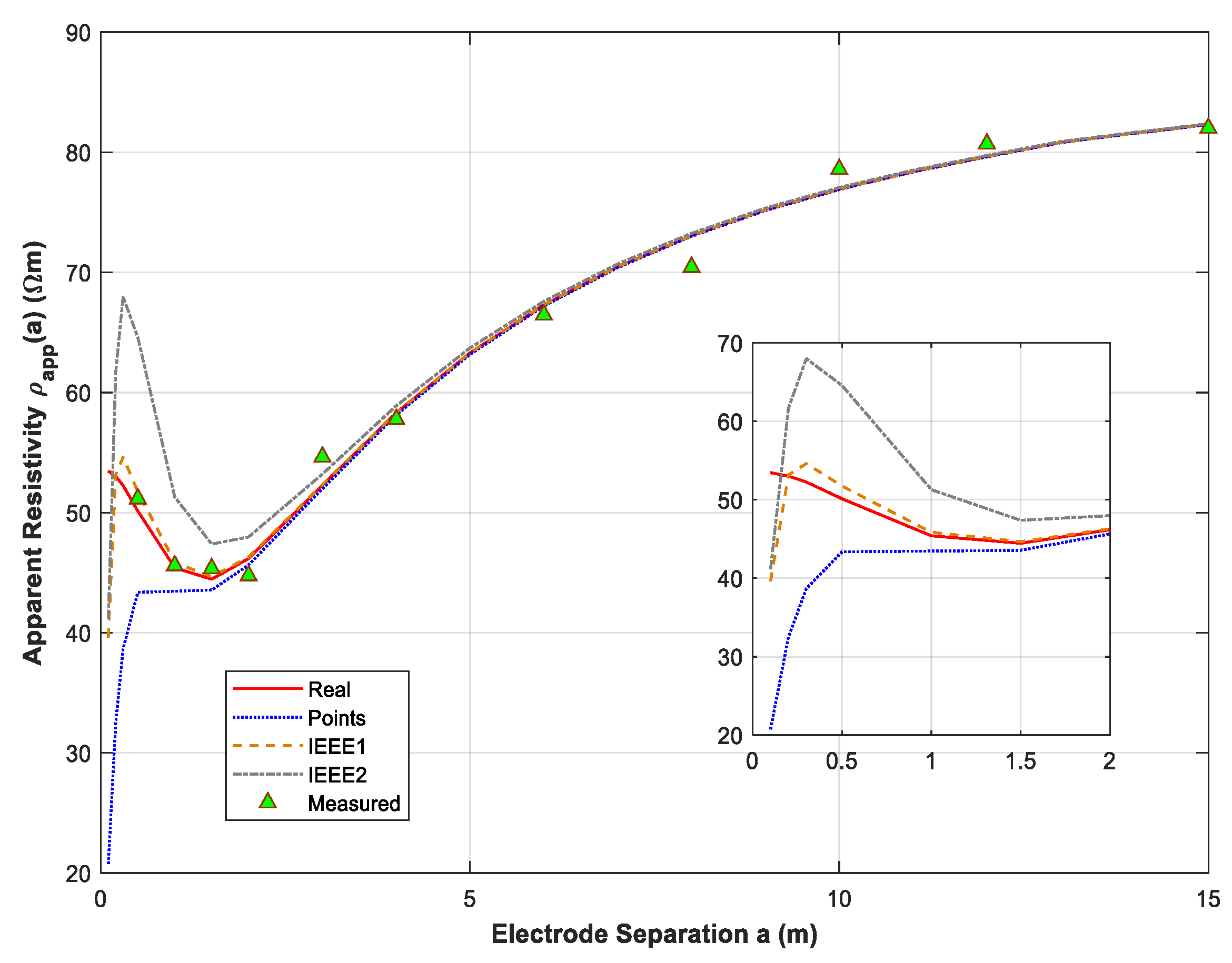
3.2. Case Study 2
3.3. Case Study 3
4. Conclusions
Author Contributions
Funding
Acknowledgments
Conflicts of Interest
References
- Samouelian, A.; Cousin, I.; Bruand, A.T.A.; Richard, G. Electrical resistivity survey in soil science: A review. Soil Tillage Res. 2005, 83, 173–193. [Google Scholar] [CrossRef]
- Van Nostrand, R.G.; Cook, K.L. Interpretation of Resistivity Data; Geological Survey Professional Paper 499; USGS: Reston, VA, USA, 1966.
- Hesse, A.; Jolivet, A.; Tabbagh, A. New prospects in shallow depth electrical surveying for archaeological and pedological applications. Geophysics 1986, 51, 585–594. [Google Scholar] [CrossRef]
- Grard, R. A quadrupolar array for measuring the complex permittivity of the ground: Application to Earth prospection and planetary exploration. Meas. Sci. Technol. 1990, 1, 295–301. [Google Scholar] [CrossRef]
- Wenner, F. A Method of Measuring Earth Resistivity; Scientific Paper, Report No. 258; National Bureau of Standards: Gaithersburg, MD, USA, 1916; Volume 12, pp. 469–482.
- Jacubas, A.; Jablonski, P. The influence of electrode size on resistance measurement in the modified four-electrode method. Measurement 2017, 108, 34–40. [Google Scholar] [CrossRef]
- Sunde, E.D. Earth Conduction Effects in Transmission Systems; Dover Publications Inc.: Mineola, NY, USA, 1949. [Google Scholar]
- Olowofela, J.A.; Jolaosho, V.O. Measuring the electrical resistivity of the Earth using a fabricated resistivity meter. Eur. J. Phys. 2005, 26, 501. [Google Scholar] [CrossRef]
- IEEE Guide for Measuring Earth Resistivity, Ground Impedance, and Earth Surface Potentials of a Grounding System; IEEE Standard 81; IEEE: Piscataway, NJ, USA, 2012.
- Faleiro, E.; Asensio, G.; Moreno, J. Improved measurements of the apparent resistivity for small depths in Vertical Electrical Soundings. J. Appl. Geophys. 2016, 131, 117–122. [Google Scholar] [CrossRef]
- Takahashi, T.; Kawase, T. Analysis of apparent resistivity in a multi-layer earth structur. IEEE Trans. Power Deliv. 1990, 5, 604–612. [Google Scholar] [CrossRef]
- Harrington, R.F. Field Computation by Moment Methods; IEEE Press: New York, NY, USA, 1993. [Google Scholar]
- Seedher, H.R.; Arora, J.K. Estimation of two layer soil parameters using finite Wenner resistivity expressions. IEEE Trans. Power Deli. 1992, 7, 1213–1217. [Google Scholar] [CrossRef]
- Gupta, P.K.; Niwas, S.; Gaurz, V.K. Straightforward inversion of vertical electrical sounding data. Geophysics 1997, 62, 775–785. [Google Scholar] [CrossRef]


| Electrode | ||||
|---|---|---|---|---|
| GF | 1 | 2 | 3 | 4 |
| L (m) | 0.2 | 0.02 | 0.01 | 0.9 |
| r (m) | 0.007 | 0.01 | 0.01 | 0.005 |
| M | 20 | 2 | 1 | 30 |
| a (m) | R(a) (Ω) | F(a) (m) |
|---|---|---|
| 0.5 | 13.64 | 3.75 |
| 1 | 6.87 | 6.64 |
| 1.5 | 4.69 | 9.67 |
| 2 | 3.51 | 12.75 |
| 3 | 2.88 | 18.97 |
| 4 | 2.29 | 25.23 |
| 6 | 1.76 | 37.76 |
| 8 | 1.40 | 50.31 |
| 10 | 1.25 | 62.87 |
| 12 | 1.07 | 75.43 |
| a (m) | R(a) (Ω) | F(a) (m) |
|---|---|---|
| 0.5 | 13.81 | 3.63 |
| 1 | 6.92 | 6.57 |
| 1.5 | 4.62 | 9.62 |
| 2 | 3.63 | 12.71 |
| 3 | 2.76 | 18.95 |
| 4 | 2.32 | 25.21 |
| 6 | 1.79 | 37.75 |
| 8 | 1.45 | 50.30 |
| 10 | 1.22 | 62.86 |
| 12 | 1.05 | 75.42 |
© 2019 by the authors. Licensee MDPI, Basel, Switzerland. This article is an open access article distributed under the terms and conditions of the Creative Commons Attribution (CC BY) license (http://creativecommons.org/licenses/by/4.0/).
Share and Cite
Faleiro, E.; Asensio, G.; Denche, G.; Garcia, D.; Moreno, J. Wenner Soundings for Apparent Resistivity Measurements at Small Depths Using a Set of Unequal Bare Electrodes: Selected Case Studies. Energies 2019, 12, 695. https://doi.org/10.3390/en12040695
Faleiro E, Asensio G, Denche G, Garcia D, Moreno J. Wenner Soundings for Apparent Resistivity Measurements at Small Depths Using a Set of Unequal Bare Electrodes: Selected Case Studies. Energies. 2019; 12(4):695. https://doi.org/10.3390/en12040695
Chicago/Turabian StyleFaleiro, Eduardo, Gabriel Asensio, Gregorio Denche, Daniel Garcia, and Jorge Moreno. 2019. "Wenner Soundings for Apparent Resistivity Measurements at Small Depths Using a Set of Unequal Bare Electrodes: Selected Case Studies" Energies 12, no. 4: 695. https://doi.org/10.3390/en12040695
APA StyleFaleiro, E., Asensio, G., Denche, G., Garcia, D., & Moreno, J. (2019). Wenner Soundings for Apparent Resistivity Measurements at Small Depths Using a Set of Unequal Bare Electrodes: Selected Case Studies. Energies, 12(4), 695. https://doi.org/10.3390/en12040695