1. Introduction
With the continual enlargement in scale of power grid interconnections and the increasing large-scale integration of renewable power generation, the dynamic characteristics of power systems have become more and more complex, resulting in higher requirements for power system stability analysis [
1,
2]. In recent years, due to the wide application of wide-area measurement systems and rapid development of artificial intelligence (AI) methods, power system transient stability status prediction (TSSP) based on AI methods has attracted extensive attention. Generally, TSSP is treated as a two class classification problem, including the stable class and the unstable class [
3]. Offline, the mapping relationship between the input features and the stability status is established by using the strong nonlinear mapping abilities of AI methods. Online, the upcoming transient stability status of the system can be quickly predicted by feeding the input features into the established classification model.
The input features are important factors that affect the performance of the classification model. However, the existing feature sets applied to TSSP are often manually selected according to experience, which can significantly degrade the performance of the classification model due to the existence of irrelevant and redundant features [
4].
Feature selection, which refers to the process of filtering out the optimal feature subset from the original feature set, can eliminate irrelevant and redundant features and improve classification performance [
5]. Therefore, it has become a basic data preprocessing method, and it is of great significance to study the feature selection method for TSSP.
The existing methods for TSSP feature selection can be divided into two main categories [
6]: the filter method and the wrapper method.
The filter method ranks the original features by calculating the importance of each individual feature, and it selects a predefined number of top-ranked features as the input features for classification models. Different filter methods are generated according to different importance metrics. In [
7,
8], the Fisher criterion is utilized to evaluate features comprehensively, considering both the intra-class distance and the inter-class distance. Information measure-based feature selection methods are utilized to select important features in [
9,
10]. Other methods, such as the relief method [
11] and the rough set method [
12], are also adopted for TSSP feature selection. The filter method is computationally efficient since it ranks features individually, but it is less effective due to the lack of a classification model in the search process.
The wrapper method considers the feature selection as an optimization problem, and evaluates the feature subset by using certain search strategies and classification algorithms. Based on different search strategies, the wrapper method can be classified into the greedy search technique and the heuristic search technique. The former includes sequence forward search (SFS) methods and sequence backward search (SBS) methods, and the latter mainly includes genetic algorithms (GA) [
13], binary particle swarm algorithms (PSO) [
14], etc. Since the wrapper method combines the feature selection problem with the classification model, it often has a better performance than the filter method [
15]. However, as the feature dimension increases, the wrapper method is usually preferred to obtain the local optimal solution of the problem.
From the above analysis, it can be concluded that both the filter method and the wrapper method have their own merits and demerits, and a more effective feature selection approach should be developed for TSSP problem.
In this paper, a novel two-stage feature selection method is proposed for TSSP problem. In the first stage, normalized mutual information (NMI) is utilized for measuring the relevance between individual feature and classes, and the features are ranked based on the NMI values. Then, the top-ranked features are selected to form the strongly relevant feature subset (SRFS), and the remaining features are described as the weakly relevant feature subset (WRFS). The results obtained in the first stage will be used as the prior knowledge for the next stage. In the second stage, binary particle swarm optimization (BPSO) is utilized as the search algorithm for feature selection, and a new particle encoding strategy that considers population diversity and prior knowledge is proposed. In addition, fitness function plays a very important role in controlling the search direction of BPSO. By taking the imbalanced characteristic of the TSSP problem into consideration, an improved fitness function composed of the geometric mean index and feature subset length is proposed. In this paper, k-nearest neighbor (KNN) is chosen as the classifier to evaluate the classification performance of the candidate feature subset because of its simplicity and rapidity.
The rest of the paper is organized as follows.
Section 2 introduces the methodologies used in the paper.
Section 3 describes the process of initial feature set construction and data generation. In
Section 4, the proposed two-stage feature selection method is provided. The case study is shown in
Section 5 and the conclusion is drawn in
Section 6.
2. Methodology
2.1. Normalized Mutual Information
Mutual information represents the information shared by two variables, which can be utilized for measuring the correlation degree of two variables [
16].
Entropy is the measure of the uncertainty of a random variable. If the probabilities of different output classes
C are
P(
ci),
i = 1, …,
Nc, then the entropy
H(
c) is defined as follows:
The joint entropy of feature vector
F and output class
C is defined as:
When the feature vector
F is known, the residual uncertainty in the output class
C is measured by the conditional entropy:
The relationship between the conditional entropy, entropy, and joint entropy can be demonstrated as below:
The mutual information between two variables
C and
F is defined as [
16]:
From the above equation, it can be concluded that mutual information measures the reduction amount of class uncertainty after proving the knowledge of feature vectors.
The mutual information is symmetric and can be reduced to the following equation:
In order to normalize the mutual information value into [0, 1], the normalized mutual information (NMI) [
17] is denoted as:
The larger the NMI value is, the stronger the relevance between features and classes will be, and vice versa. If the NMI value is 0, it means that the feature vector and classes are totally irrelevant or independent of each other. If the NMI value is 1, it indicates that the feature vector and classes are completely relevant.
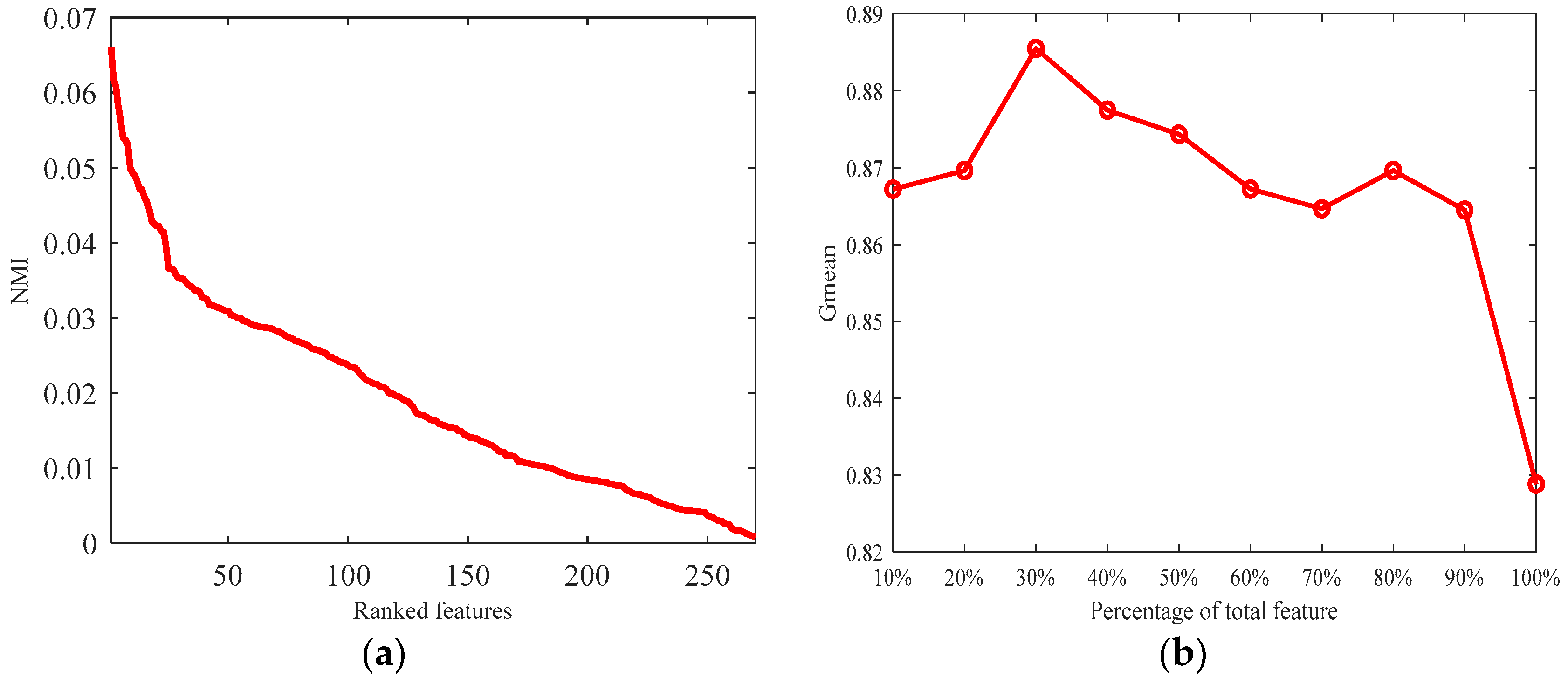
After ranking the features based on the NMI values, the predefined number of top-ranked features can be selected to form the SRFS, and the remaining features are described as WRFS.
2.2. Binary Particle Swarm Optimization
Among the heuristic intelligent optimization algorithms, the particle swarm optimization (PSO) algorithm, which is easy to implement and has few parameters to tune, is superior to other algorithms in terms of success rate and solution quality. The binary version of PSO (BPSO) is employed for TSSP feature selection since it is a discrete optimization problem with binary solution space [
18].
In BPSO, every possible solution to this optimization problem is presented by a particle, which has the two attributes of position and velocity. The next particle velocity is determined by the current particle velocity and particle position. Specifically, during each iteration, particles will be updated based on the distance from the individual best position and the distance from the global best position. The velocity updating formulas of PSO are provided as follows:
where
and
are velocity and position of the particle
i in dimension
d at iteration
k, respectively;
pbest indicates the best position of the particle
i in dimension
d at iteration
k, while
gbest is the best position in the swarm so far;
c1 and
c2 represent the acceleration coefficients;
r1 and
r2 are the random numbers from a uniform distribution within the range of [0, 1]. The inertia weight
ω is used to control the impact of the last velocity to the current velocity, which is linearly decreased from
ωmax to
ωmin to balance the global and local search [
19], as shown in Equation (9).
Nk is the maximum number of iterations.
The particle position in BPSO algorithm is updated based on the velocity value, and the transfer function should be employed to map the real valued velocity to a probability value between [0, 1] to change the binary position.
The velocity value in the BPSO algorithm means the difference between the current particle and the optimal particle. If the absolute value of velocity is relatively large, it means that the difference between the current particle and the optimal particle is large, and at this time, the transfer function should provide a higher possibility to change the position status of the current particle. Conversely, if the absolute value of the velocity is small, the difference between the current particle and the optimal particle is small. Then the transfer function should provide a higher probability to maintain the current position status. Therefore, v-shaped transfer functions designed in [
20,
21] is utilized for converting the velocity value to the changing probability of position status, as shown below:
After calculating the probability value, the binary position is then updated with the following formula:
where
r3 is a random number uniformly distributed between [0, 1].
According to Equation (11), the particle position will be changed to the opposite status when the random number is smaller than , and when the random number is larger than , the status of particle position will be maintained.
The main steps of BPSO for solving binary optimization problem are describe below:
- Step 1:
Set the parameters of BPSO including population size, maximum iteration number, velocity range, learning factors, and inertia weight range.
- Step 2:
Initialize the binary position and velocity of each particle randomly.
- Step 3:
Calculate the fitness function of each particle, and update the values of individual best position pbest and global best position gbest.
- Step 4:
Update the velocity by using Equation (8) and the binary position by using Equations (10) and (11).
- Step 5:
Terminate the optimization process when the maximum iteration number is reached, and go on to step 6. Otherwise, increase the iteration number and return to step 3.
- Step 6:
Save the global best position as the ultimate solution for the binary optimization problem.
2.3. New Particle Encoding Strategy
Before using the heuristic search method for feature selection, the population initialization should be carried out first.
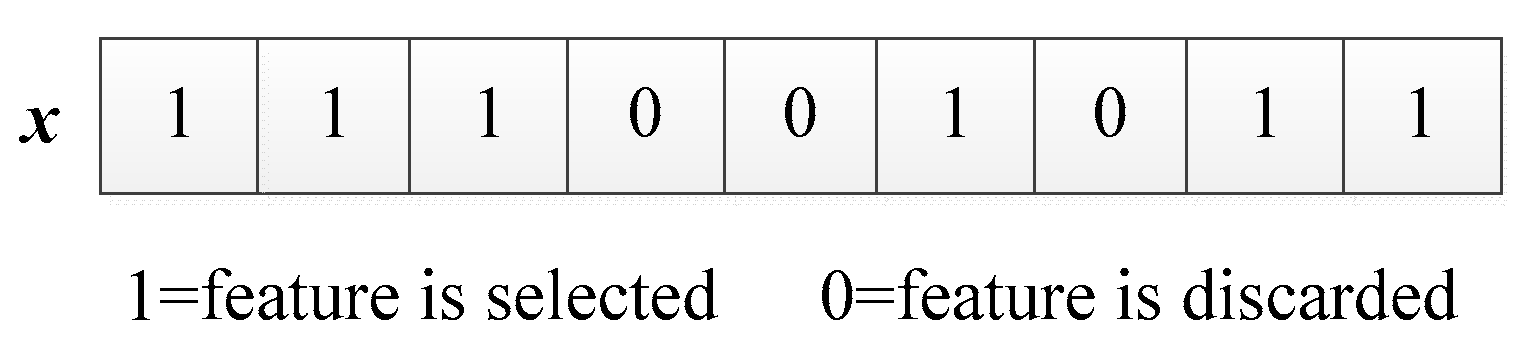
Figure 1 is an encoding schematic diagram of a particle with 9-dimensional features, where 1 indicates that the feature is selected, and 0 indicates that the feature is discarded.
The binary status of the dimension
d of particle
i is encoded by the following formula:
where
r4 is a random number uniformly distributed between [0, 1], and
p is a value between [0, 1].
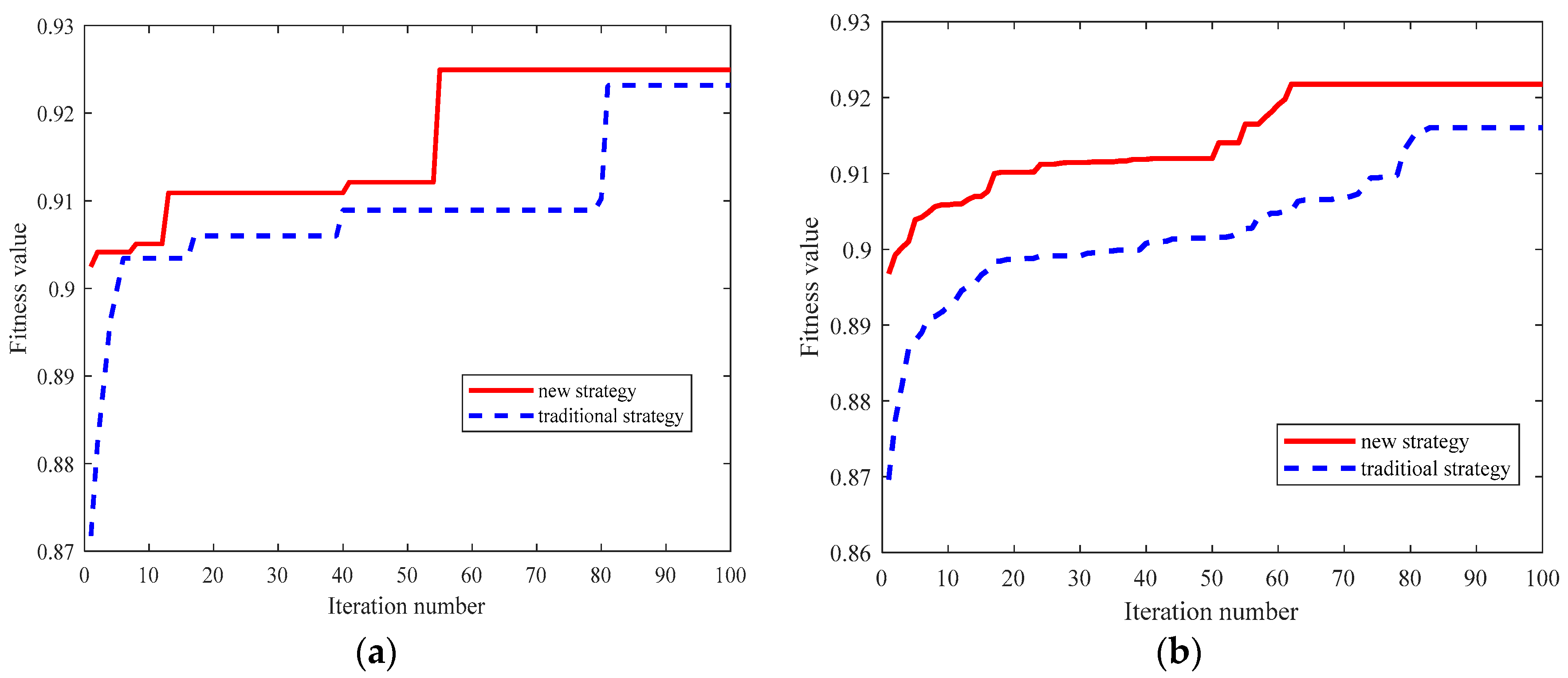
The value of p indicates the probability that the dimension d is set to 1. In the conventional particle encoding method, each feature is selected by a completely random way, and the p is set to 0.5. The advantage of this particle encoding method is that it can increase the population diversity, but the disadvantages are that it can slow down the convergence speed and easily lead to local optimal solution, especially when the dimensions of feature selection problem is large.
As described in
Section 2.1, the initial feature set can be divided into SRFS and WRFS based on the value of NMI. A feature in SRFS means that this feature has a higher probability to be chosen as the ultimate input feature, and a feature in WRFS means that this feature has a lower probability to be chosen as the ultimate input feature. The information obtained in
Section 2.1 can be embedded into the particle encoding process as prior knowledge, which can guide the search direction of particles, and improve the efficiency and effectiveness of the feature selection results.
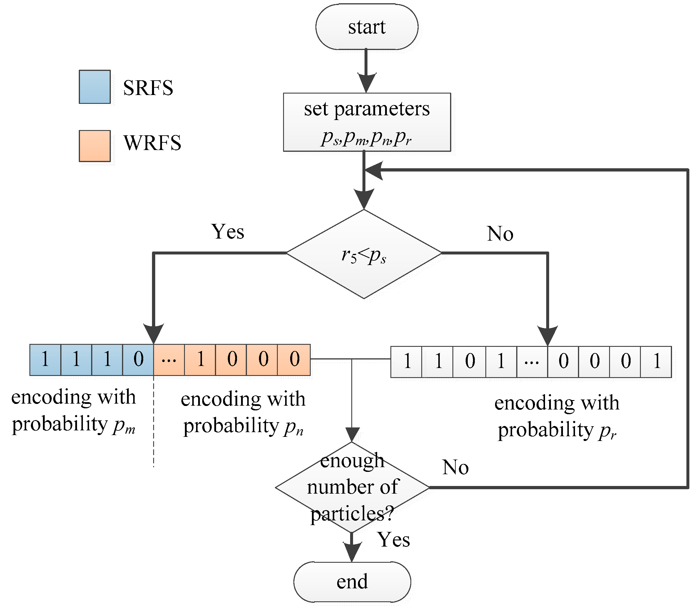
Based on the analysis above, a new particle encoding strategy considering the population diversity and priori knowledge is proposed, whose flowchart is shown in
Figure 2.
From
Figure 2, the main steps of the proposed particle encoding are listed below:
- Step 1:
Generate a random number r5 uniformly distributed in [0, 1], and compare the random number with ps. If the random number r5 is smaller than ps, go to step 2; otherwise, go to step 3. The value of ps determines the proportion of completely random particle encoding and the particle encoding with prior knowledge, and ps is set to 0.5 in this paper to balance two different particle encoding methods.
- Step 2:
Encode the particles considering the prior knowledge which is obtained from Step 1. For the feature in SRFS, the value of p in Equation (12) is set to pm, and the pm is bigger than 0.5, meaning that these kinds of features have higher probabilities to be selected. For the feature in WRFS, the value of p in Equation (12) is set to pn = 1 − pm, meaning that the pn is smaller than 0.5 and these kinds of features have higher probabilities to be discarded. Then, go to step 4.
- Step 3:
Encode the particles in a completely random way. All the features are encoded with the original way, meaning that the value of pr is set to 0.5, and each feature has the same probability to be selected. The purpose of this operation is to increase the diversity of populations. Then, go to step 4.
- Step 4:
Check whether the number of particles is enough. If yes, stop the particle encoding process, otherwise, back to step 1.
2.4. Geometric Mean (Gmean)-Based Fitness Function
For TSSP feature selection, classification performance and feature number are two inevitable aspects which should be taken into consideration in fitness function. In the existing research, the overall classification accuracy (OCA) is always utilized as the index of classification performance. However, since power systems are scheduled to operate under stable conditions most of the time, the sample numbers of stable class and unstable class are usually highly imbalanced [
13]. In this situation, the OCA tends to obscure the classification performance of the unstable class with a small sample number, which does not meet the actual operational requirements of the power system. Therefore, it is not suitable to use the OCA as the classification performance index for TSSP feature selection.
In general, the classification performance of TSSP can be represented by a confusion matrix, which is shown below.
In
Table 1,
TS represents the sample number of stable classes classified as stable class,
TU represents the sample number of unstable classes classified as unstable class,
FU represents the sample number of stable classes misclassified as unstable class, and
FS represents the sample number of unstable classes misclassified as stable class.
The true stable class rate (TSR) represents the proportion of the sample number of stable classes truly classified as stable class in the total number of stable classes, as shown below:
The true unstable class rate (TUR) indicates the proportion of the sample number of unstable classes truly classified as unstable class in the total number of unstable classes, as shown below:
To cope with the class-imbalance problem of TSSP, the geometric mean (Gmean) [
22,
23] of TSR and TUR is employed as the overall performance of classification model in lieu of conventional classification accuracy, which can be expressed as:
It can be seen from the above formula that the larger the Gmean is, the better the classification performance will be. When both TSR and TUR are 1, Gmean is 1.
In order to further illustrate that Gmean is more suitable for evaluating classification model performance than the traditional accuracy for TSSP, comparison of these two indexes are done below.
The formula of OCA can be expressed as below:
where
Ns,
Nu, and
N are the sample number of stable class, the sample number of unstable class and total sample number, respectively.
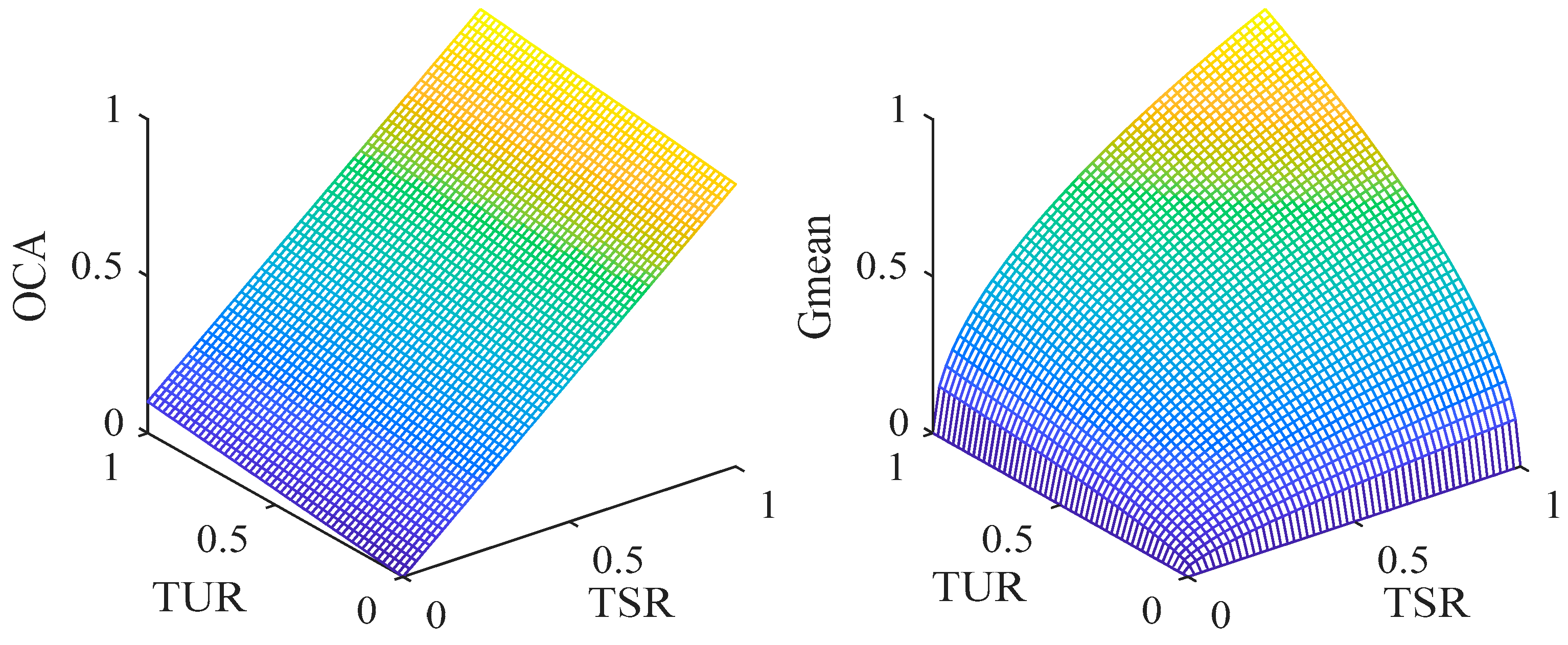
The OCA index can be considered as the linear weighting of TSR and TUR, and the weight factor is related to the sample number of stable class and unstable class. Assuming that the sample number ratio of stable class and unstable class is 9:1, the comparison of OCA and Gmean is shown in
Figure 3.
It can be seen from the
Figure 3 that OCA is biased toward stable class classification performance, which has more samples, and Gmean is not biased towards the classification performance of stable class and unstable class since it is independent of the sample number. Specifically, when TUR is 0 and TSR is 1, OCA is about 90%, but Gmean is 0. Therefore, Gmean is more suitable for evaluating TSSP classification performance than OCA.
Considering both the TSSP classification performance and the number of features, the Gmean-based fitness function is defined below:
where
NC is the number of selected features and
NF is the total number of features.
λ is the weight factor to balance these two terms, which is very small to ensure that the classification performance is more important than feature subset length.
4. Proposed Two-Stage Feature Selection Method
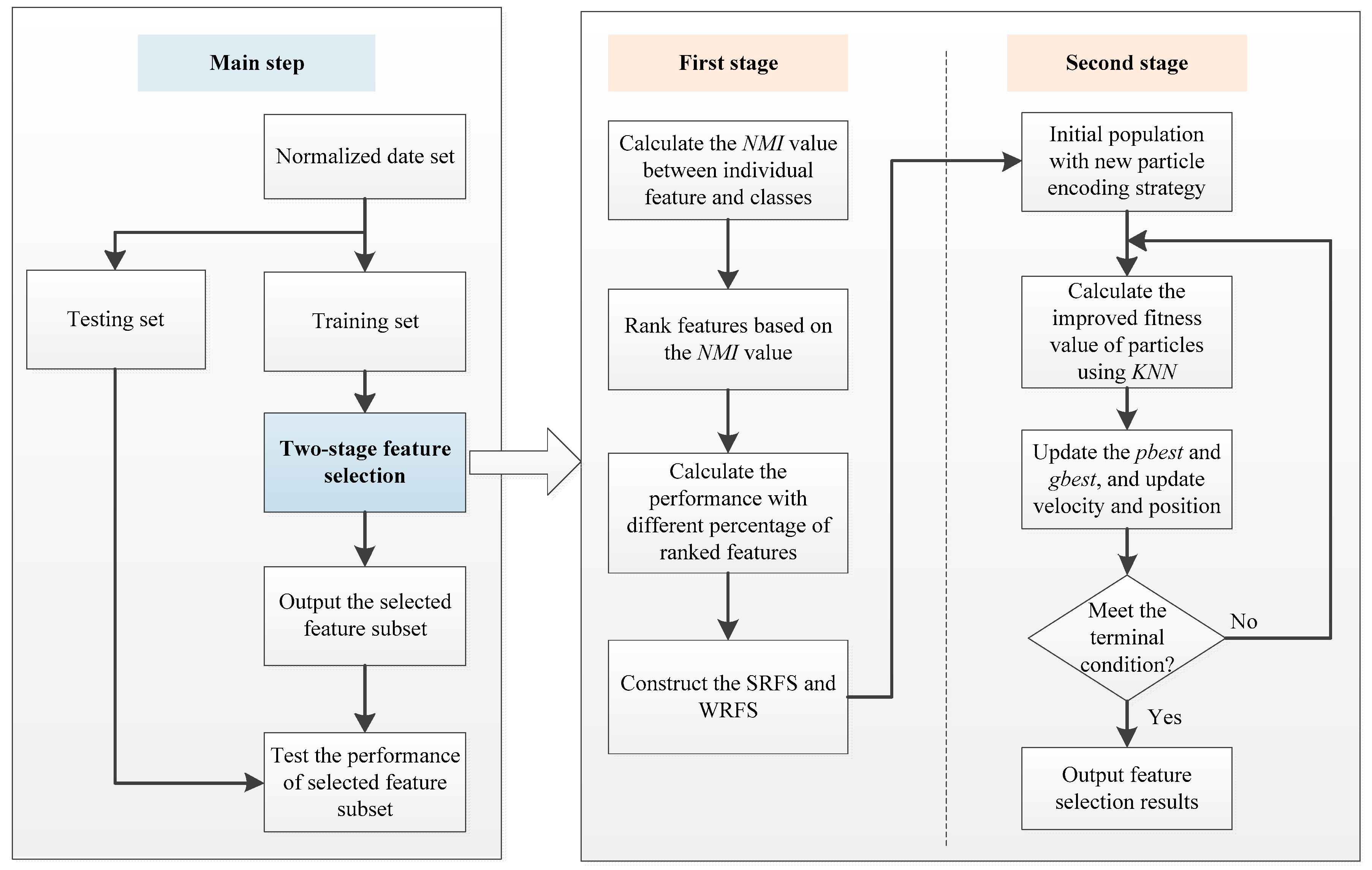
In this section, two-stage feature selection method for the TSSP problem is proposed, which is described briefly below.
The collected data is normalized and randomly divided into training set and testing set. The training set is employed for feature selection and the testing set is utilized to check the quality of the selected feature subset.
In the first stage, the NMI value is calculated with the training set and utilized for measuring the relevance between features and classes, and the features are ranked from large to small based on the NMI values. Then, the classification performance of the ranked features is calculated by using the KNN model to determine the SRFS and WRFS.
In the second stage, the population of BPSO is initialized with the new particle encoding strategy, and the improved fitness value of the particle is calculated with KNN. The values of individual best position and global best position are updated, and the velocity and binary position of particles are updated. The above process is repeated until the terminal condition is met.
After finishing the feature selection process, the classification performance of the selected feature subset is calculated on the testing set.
The flowchart of the proposed two-stage feature selection method is depicted in
Figure 4.
6. Conclusions
This paper proposed a new two-stage feature selection algorithm for TSSP. In the first stage, all the features are divided into SRFS and WRFS based on the NMI values, and in the second stage, a new particle encoding strategy considering both population diversity and prior knowledge is presented. Additionally, considering the imbalanced characteristics of TSSP, an improved fitness function is utilized. The following conclusions can be made from experimental results: (1) compared with the traditional completely random particle encoding method, the proposed particle encoding method can obtain better feature selection results, (2) compared with the OCA-based fitness function, the proposed Gmean-based fitness function tends to select the feature subset having stronger recognition ability for unstable class, and (3) compared with some state-of-the-art feature selection methods, the proposed two-stage feature selection achieves significantly better performance results in terms of TUR and Gmean, and similar results in TSR, which shows that the proposed feature selection method is more suitable for actual power system TSSP problem.
Future work will focus on the improvement of classification model to better handle the imbalanced characteristics of power system TSSP problem.


