Abstract
The cross-entropy based hybrid membrane computing method is proposed in this paper to solve the power system unit commitment problem. The traditional unit commitment problem can be usually decomposed into a bi-level optimization problem including unit start-stop scheduling problem and dynamic economic dispatch problem. In this paper, the genetic algorithm-based P system is proposed to schedule the unit start-stop plan, and the biomimetic membrane computing method combined with the cross-entropy is proposed to solve the dynamic economic dispatch problem with a unit start-stop plan given. The simulation results of 10–100 unit systems for 24 h day-ahead dispatching show that the unit commitment problem can be solved effectively by the proposed cross-entropy based hybrid membrane computing method and obtain a good and stable solution.
1. Introduction
The unit commitment (UC) problem is a typical optimization problem for power systems. The main goal of UC is to schedule the start-stop state of units and generate power according to the load forecasting curve during the dispatch period, with the corresponding constraints so that the cost is minimized [1]. Usually the UC problem can be broken down into two sub-problems: the unit start-stop plan and economic dispatch [2].
Mathematically, the UC problem is a high-dimensional, non-convex and mixed-integer nonlinear programming problem. Its discrete and continuous variables, non-convex objective function and network constraints enhance its non-convexity and complex [3]. Moreover, with the increase in unit and calculation scale, it is difficult to obtain an accurate feasible solution in a reasonable time frame. Therefore, many methods have been proposed by scholars to solve the UC problem, which can be roughly divided into three categories: heuristic methods, mathematical optimization methods, and intelligent optimization methods.
Heuristic methods are represented by the priority list method [4], the earliest method applied to solve the UC problem, which generally sorts by some economic indicators with small and simple calculations, usually relies on the actual scheduling experience.
Mathematical optimization methods include mixed integer nonlinear programming, the Lagrangian relaxation (LR) method [5], etc. Mixed integer nonlinear programming methods include the branch-and-bound (BB) [6], Benders decomposition [7], and other methods, with the decomposition technique generally used to simplify the problem; the solving efficiency has been rapidly improved with improvements in mathematical optimization software [8]. For the dynamic programming method, the global optimal solution can be obtained with no special requirements on the behavior of the objective function; however, there will be a “dimensionality disaster” [9] when the number of units is large, and to simplify the problem, the optimal solution will be lost when the approximation method adopted. Moreover, it is difficult to consider time-dependent constraints such as the ramp rate constraint. Compared with the dynamic programming method, the LR method has an advantage for large-scale problems since the calculation complexity is approximately proportional to the unit scale; in addition, the Lagrangian multiplier is of practical economic significance, but it cannot prove whether the solution is optimal due to the dual gap. It is also inflexible when considering some kinds of constraints, such as the ramp rate limit, and the possible oscillation and singularity during iteration may lead to convergence difficulties [10].
Bioinspired optimization methods are algorithms that simulate biological evolution or its behavior, and include genetic algorithms (GA) [11], particle swarm algorithm (PSO) [12], and memetic algorithm (MA) [13]. An approximate optimal solution can be obtained with no special requirements on the behavior of the objective function, and feasible solutions can be obtained even when the unit scale is large where no feasible solution can be obtained by other methods; however, the solving efficiency is affected by how the constraints are processed since these methods are essentially unconstrained.
Membrane computing is a computational framework inspired by the living cell and its organization in tissues and other higher order structures, and was first proposed by Gheorghe Pǎun, an academic at the European Academy of Sciences. In recent years, optimization problems such as image processing [14], robot path planning [15], DNA sequence design [16], gasoline blending scheduling [17], the travelling salesman problem [18], and the minimum storage problem [19] have been successfully solved by this framework. In this paper, we propose a cross-entropy-based hybrid membrane computing (CEHMC) method to solve the UC problem by combining the genetic algorithm-based P system (GAPS) with the biomimetic membrane computing (BMC) method. The GAPS is based on the binary genetic algorithm. It is nested by multiple membranes with the unit start-stop state (0,1 binary variables) as evolution objects. The evolution rules adopt the crossover and mutation rules of binary coded genetic algorithms. The difference between GAPS and GA is the communication of optimal objects in different membranes, which means the optimization results of the outer membrane can be transmitted into the inner membranes constantly when genetic rules are executed in each membrane. The calculation method of biomimetic membrane is inspired by the important role of Golgi apparatus in living cells. With the inner membrane system as the calculation carrier, the required regional structure is designed to simulate the static or dynamic membrane structure, the biochemical or physical reactions in the inner membrane system are simulated by various evolutionary rules, so that the top-ranking evolution objects after evaluation are selected for transmission according to the permeability of substances in the transporting through the membrane. Based on the combination of GAPS with the biomimetic membrane computing method, the cross-entropy (CE) optimization method is introduced to strengthen the searching ability during the optimization.
Because the UC problem is not fully standardized and specified, we will not attempt to give a definitive algorithmic solution to the problem. Instead, our goal in this paper is to demonstrate that the proposed CEHMC approach is viable. We include a case study showing than our method outperforms other nonlinear optimization alternatives for a case study. Therefore, our formulation of the UC problem and its solution algorithm are for illustration purposes only. For that purpose and for the ease of exposition and understanding, the classical UC formulation which has been commonly used in the past decades is used in this paper. The simulation results of 10–100 unit systems for 24 h day-ahead dispatching showed that the UC problem could be solved effectively by the proposed method, and a satisfactory and stable solution was obtained.
2. The Mathematical Model for UC Problems
2.1. Objective Function
The total generation cost FC during the dispatching period is taken as the optimization goal, including fuel cost and startup cost of all units. Thus, the objective function is:
where T is the total dispatch period; N is the number of generators; Ii,t is the state of unit i at tth hour; value 1 represents startup, while 0 represents shutdown; Fi,t and Ci,t are the fuel cost and startup cost, respectively, of unit i at t-th hour; and the fuel cost Fi,t can be expressed by the quadratic function as follows:
where Pi,t is the generation of unit i at t-th hour; and Ai,2, Ai,1, and Ai,0 are the unit cost coefficients of unit i.
Startup cost Ci,t is related to the unit OFF time, which can be expressed by the following step function:
where Chot,i and Ccold,i are the hot start cost and cold start cost, respectively, of unit i; is the minimum downtime of unit i; is the OFF time of unit i at t-th hour; and is the cold start time of unit i.
2.2. Constraints
The constraints of the UC problem usually include the system power balance, system spinning reserve requirement, generation limits, ramp rate limits, and minimum up and down time limits.
- System power balance:
- System spinning reserve requirement:
- Generation limits:
- Ramp rate limits:
- Minimum up and down time limits:
Here, Dt is the system load demand at t-th hour; and are the maximum and minimum generation limits, respectively, of unit i; Rt is the system reserve demand, typically 5–10% of the system load demand; and are the up and down ramp rate limit, respectively; and are the start and stop rate limit, respectively; is the OFF time of unit i at the (t−1)-th hour; and is the minimum up time.
3. Unconstrained UC Model for CEHMC Method
As mentioned above, the traditional UC model is a multi-constrained nonlinear optimization problem, yet natural computing frameworks such as membrane computing are essentially unconstrained optimization methods, which are commonly used to solve unconstrained optimization problems. As for the complex multi-constrained optimization problem, using the penalty function is usually a good choice [20]. To facilitate the proposed method, the quadratic penalty function was used to deal with the constraints, transforming the UC problem into an unconstrained model without providing any initial feasible solution. Since GAPS is for the unit start-stop plan with embedded generic rules. These rules are design to screen the unit start-stop plans, i.e., testing whether the system spinning reserve requirement and minimum up and down time limits are satisfied, which determines the feasible unit state combination. Consequently, for the unconstrained UC model, only system power balance and ramp rate limits need to be transformed. The objective function can be rewritten as a penalty function as follows:
Here, the penalty factors μ1, μ1 > 0; δ > 0 is the acceptable violation domain when converting the equality constraint into an inequality constraint. In fact, the value of penalty factors is related to the magnitude of objective function and constraints. If the value is too large, it is likely to get bad solutions, and if the value is too small, the searching direction might be far away from the feasible region. Therefore, the method of testing is usually used to make the penalty item have the same or larger magnitude as the objective function so as to determine the penalty factors.
4. CEHMC Method Applied to Solve UC Problem
Three basic elements of membrane computing are membrane structure, evolution object, and evolution rules. The membrane structure and evolution rules can be designed according to requirements [21]. Taking an intracellular membrane system as the computational framework, the main procedures of the membrane computing method are as follow: first design the membrane structure, then evolve objects according to evolution rules, and lastly select the optimal objects for transmission and communication.
When using the CEHMC method for solving the UC problem, we utilize GAPS to schedule the unit start-stop plan since the start-stop states of generators are discrete variables. While for the dynamic economic dispatch problem, the generation of units is a continuous variable. Since the evolutionary objects (solution vectors) of biomimetic membrane computing is only required to be a real number, not limited to discrete variables. If the evolutionary rules are set to apply to continuous variables, biomimetic membrane computing can used to solve continuous variable optimization problems, such as the dynamic economic dispatch problem in UC. Then, the cross-entropy optimization method is introduced combined with biomimetic membrane computing to improve the searching ability during iteration. Finally, the minimum generation cost is taken as the optimal result of the UC problem.
4.1. GAPS for Unit Start-Stop Plan
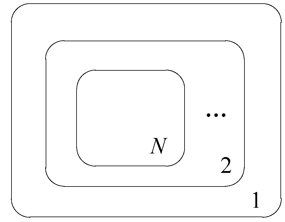
Figure 1 shows the membrane structure of GAPS; it is a nested structure [22], where the symbol N represents the N-th nested genetic membrane (i.e., the variable N in Table 1). In practice, it needs to be determined synthetically according to unit size, number of constraints, calculation time and convergence effect, etc. The start-stop states of generators are taken as the evolution objects I, and the crossover and mutation rules of the binary encoding GA are the evolution rules.
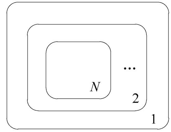
Figure 1.
Structure of genetic membrane.

Table 1.
Initial parameters of the proposed method.
4.2. Biomimetic Membrane Computing Method for Dynamic Economic Dispatch
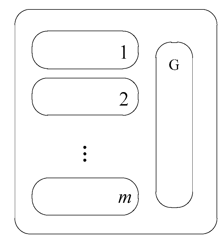
Figure 2 shows the membrane structure of the biomimetic membrane computing method used in this paper. It is a reticular structure including an outermost membrane, m basic membranes, and a quasi-Golgi membrane [23] represented by G, and the output of generators is taken as the evolution objects P, that is, , . In addition, m is corresponding to the variable Nb in Table 1, which is usually determined synthetically according to unit size, number of constraints, calculation time and convergence effect, etc.

Figure 2.
Structure of biomimetic membrane.
The evolution rules can be divided into two categories according to the environment, that is, rules in the basic membranes, and rules in the quasi-Golgi membrane. Besides, correction rules can be used in all conditions. All the basic rules are set with the calculation probability as the execution condition. When the calculation probability is satisfied, the rule will be executed immediately. The evolution rules are as follows:
1) Crossover rules
- Numerical crossover rule. Each element on both evolution object is numerically crossed, and the cross ratio of each element is different, which can be described as follows:where and are the original and new object, respectively, generated after executing evolution rule; and is a vector whose value is a random number uniformly distributed on [0,1].
- Interval crossover rule. First, select the interval to be randomly exchanged, and then swap the elements in the same interval for two objects. This is described as follows:where , is the interval to be swapped; and is the length of object. The procedure of crossover can be divided into two or three steps according to the length of the object. When the length is short, two-step crossover is preferred: first, execute the numerical crossover rule on two selected adjacent objects, and then execute the interval crossover rule on two randomly selected objects. Conversely, when the length of object is long, three-step crossover is preferred: first, execute the numerical crossover rule on two randomly selected objects, then execute the interval crossover rule on the two objects, and lastly execute the numerical crossover rule on two adjacent objects.
2) Mutation rule
A random increment vector is added to the original object, which can be described as follows:
where is the mutation vector; and are the upper and lower limits of , respectively; h is the mutation coefficient; and is the random vector that follows the standard normal distribution.
3) Correction rule
After some certain rules, such as the mutation rule, some elements of the new object may exceed their limits and must be modified, that is:
For the quasi-Golgi membrane, activation conditions are set, which means the following rules are executed only if the quasi-Golgi membrane is activated:
• Target indication rule
The communication objects sent into the quasi-Golgi are sorted by their function value, and then each communication object is subtracted from the former stored object by this order. Thus, a direction vector is generated, and the new target indication vector is the sum of this direction vector and last target indication vector. Regardless of whether the quasi-Golgi is activated, the direction vector and target indication vector should be calculated, and the target indication vector should be reserved. Furthermore, the target indication object can be generated only if the quasi-Golgi is activated. This is described as follows:
where is the target indication vector; and are the sorted communication objects stored in the quasi-Golgi this time and the last time; and both are the new target indication objects; and w is the indication coefficient.
• Transition rule
First select two elements of the selected object randomly, and then swap these elements if they are in the range of the other’s value, that is:
• Abstraction rule
The abstraction rule is designed only for optimal and suboptimal objects, where each element of the optimal object is replaced by the element on the same position of the suboptimal object, one after another. Then, the element from the suboptimal object is reserved if the new object is better than the old optimal one; otherwise, the old optimal object remains:
When using the biomimetic membrane computing method, there is an iterative calculation and communication for each basic membrane, and the good objects in the basic membrane can be reserved and sent to the quasi-Golgi for local optimization and evolution. However, with the increment of unit scale, the searching ability and stability of the method is reduced, and thus we added the CE optimization method to the membrane computing method to enhance its searching ability and stability.
4.3. CE Optimization Method
The CE method is an optimization method proposed by Rubinstein and Kroese, who estimated probabilities of rare events for stochastic networks [24]. It was first used to solve combinatorial optimization problems, and then also applied to solve continuous optimization problems [25]. Cross-entropy is a measurement for the similarity degree of two probability distributions. The main idea of CE is to get a probability distribution whose difference with the unknown optimal probability distribution is minimal [26].
For the dynamic dispatch problem:
where γ* represents the optimization result of γ for economic dispatching; is the probability space. Obviously, Equation (17) is a minimization problem. When generation obeys the distribution of , the original optimization problem can be transformed into an optimization problem of finding the optimal probability density function . Moreover, when we define as a set of different indicator functions on with value , the optimization problem of can be further transformed into a corresponding probability estimation problem as follows. The indicator functions in is used to describe the characteristics of a stochastic process, usually formulated as mean function, variance function and correlation function, etc.:
where and are the probability measure and expectation, respectively, of the optimal probability distribution .
Usually the importance sampling method is used to calculate : sampling the generation based on the probability distribution g on P:
when the probability distribution g is:
where is the value of l after the importance sampling method; g* is the assumed value of g for the importance sampling method.
There is an unbiased estimated zero variance with only one sample needed. Therefore, it is difficult to calculate since its value is related to , and the probability distribution g can usually be selected from the probability distribution cluster . In this way, the original optimization problem is finally transformed into a determination of parameter that minimizes the difference between the probability distribution of generation and optimal . In this paper, parameter includes the mean value and standard deviation of samples.
Relative-entropy (i.e., Kullback-Leibler distance) and cross-entropy are commonly used measures for the similarity degree of two probability distributions [27]. In this paper, we used the CE method, as the following formula shows:
Combining Equations (18) and (20), can be calculated by Equation (22):
Moreover, through the smoothing technique, the parameter estimation form of can be expressed as follows:
where “~” represents the parameter of elite samples. The top-ranking dispatching solutions after evaluation are chosen as the elite samples. “^” represents the parameter of total samples. is the smoothing factor (typically between 0.7 and 1); and is the value of the elite sample after the kth smoothing. Therefore, it is easier to approach the optimal solution with the correction of through the elite sample.
In short, when using the CE optimization method, first predefine the parameter and generate the candidate solution set according to the probability density function , and then update the value of through the elite sample. Thus, the searching direction continues to approximate the optimal solution in the iteration.
4.4. Procedures of CEHMC Method for UC Problem
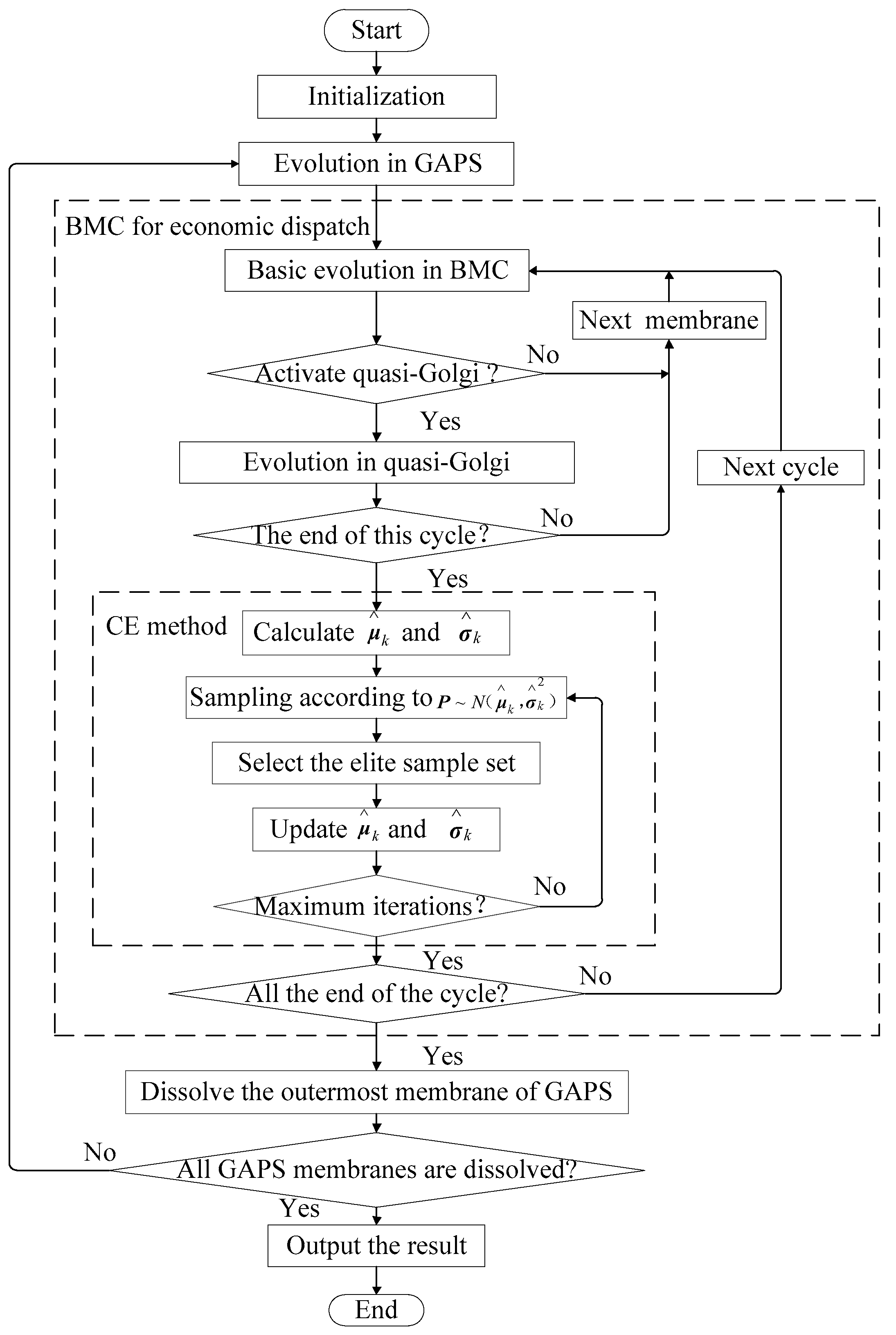
The main steps of the CEHMC method are in detail as follows, and illustrated in Figure 3.
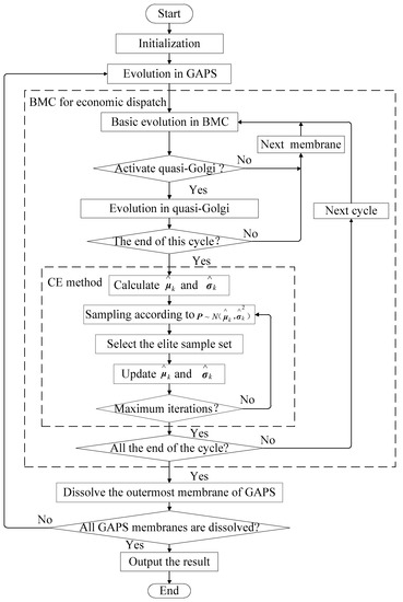
Figure 3.
Flowchart of cross-entropy-based hybrid membrane computing (CEHMC)-based unit commitment (UC) problem.
Step 1: Initialization. Set the initial parameters, construct the genetic membrane structure, and generate the initial binary object Io in each membrane (i.e., generate the start-stop states).
Step 2: Evolution. Execute the evolution rules for all objects I in each membrane.
Step 3: Evaluation. For all start-stop states, solve the economic dispatch part with the CEHMC method. The numerical result F(P) is taken as the evaluation indicator to replace the old objects. In this dispatch part, the evolution object P is the generation of units, and the main steps are as follows:
- 3.1
- Initialization. Set the initial parameters, construct biomimetic membrane structure, and create Nco initial communication objects Pco in the outermost membrane and send them to the first basic membrane.
- 3.2
- Computation in the basic membrane. Create No initial objects Po in the current membrane, and execute the basic evolution rules in order for No optimal objects to be selected in this membrane. Then, select Nco optimal objects Pbest as the communication objects Pco and Ns suboptimal objects as the reservation objects. Finally, remove the remaining objects, and send the communication objects Pco into the quasi-Golgi membrane.
- 3.3
- Computation in the quasi-Golgi membrane. Update the target indicator vector, and check whether the activate condition of quasi-Golgi is satisfied. If not, the communication objects Pco are sent to the next basic membrane directly, and return to step 3.2; if satisfied, execute evolution rules in the quasi-Golgi for communication objects Pco, and then select the new communication objects Pco.
- 3.4
- Check whether the current computation cycle is completed. If not, send the communication objects Pco into the next basic membrane and return to step 3.2; if completed, start the CE optimization steps:
- Initialization. Calculate the mean and standard deviation for all communication objects Pco in the current cycle as the initial sample.
- Sampling. Take generation samples based on the .
- Evaluation. Select the elite sample set, and then calculate its mean and standard deviation.
- Update parameters. Update the mean and standard deviation according to Equations (24) and (25):The standard deviation is usually updated by dynamic smoothing, that is, , where is the smoothing factor (typically between 0.8 and 0.99), k is the iteration number, and r is an integer (typically between 5 and 10).
- Judgment of the termination condition. If the iteration was over, output the optimal object Pbest; if not, return to Step 3.2.
- 3.5
- Judgment of termination conditions. Check whether all computation cycles are completed. If not, send the communication objects Pco to the first basic membrane and return to step 3.2; if completed, output the function value of the optimal object Pbest.
Step 4: Communication. Select Ne optimal objects Ibest, and send them to the adjacent (sub-outer) membrane. At the same time, the outermost membrane is dissolved, and thus the previous sub-outer membrane becomes the new outermost membrane.
Step 5: Judgment of termination conditions. If all membranes are dissolved, output the best result Ibest of the UC problem; if not, return to Step 3.2.
5. Case Study
The 10-unit 24 h standard thermal power test system was taken as the test example to verify the effectiveness of the proposed method. The unit characteristics and load demand are detailed in the literature [28], and the ramp rate limits of units 1, 3, and 4 are all as follows [29]: Piup = Pidown = 40 MW/h, Pistart = Pishut = 2Pi. The initial parameters of the proposed method are list in Table 1. The quasi-Golgi activate condition is that the multiplication of current computation cycle and current basic membrane can be divided by 3 after the second computation cycle.
In order to analyze the performance of the proposed method, 20 complete independent simulations are conducted on each system. Two cases of the UC problem are simulated: (1) UC problem without ramp constraints; (2) UC problem with ramp constraints. The characteristics, including the number of continues and integer variables and number of constraints for these two cases are list in Table 2, which contribute to depict the magnitude and complexity of the investigated UC problem.
Table 2.
Computation characteristics of the UC problem.
In the following sections, the corresponding simulation results for these two cases are discussed and compared. Moreover, the simulation of the proposed method is programmed by MATLAB 2014a (The MathWorks, Inc, Natick, MA, USA) on the PC with Intel Core i5-3470 CPU, 3.20 GHz, 4 GB Ram (Intel, Santa Clara, CA, USA).
5.1. Simulation Results of UC Problem without Ramp Constraints
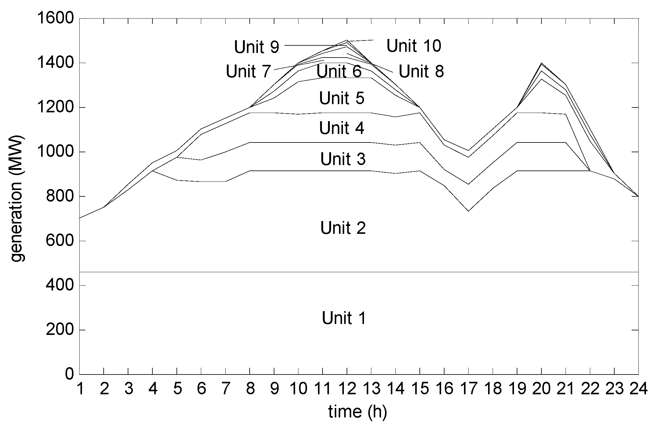
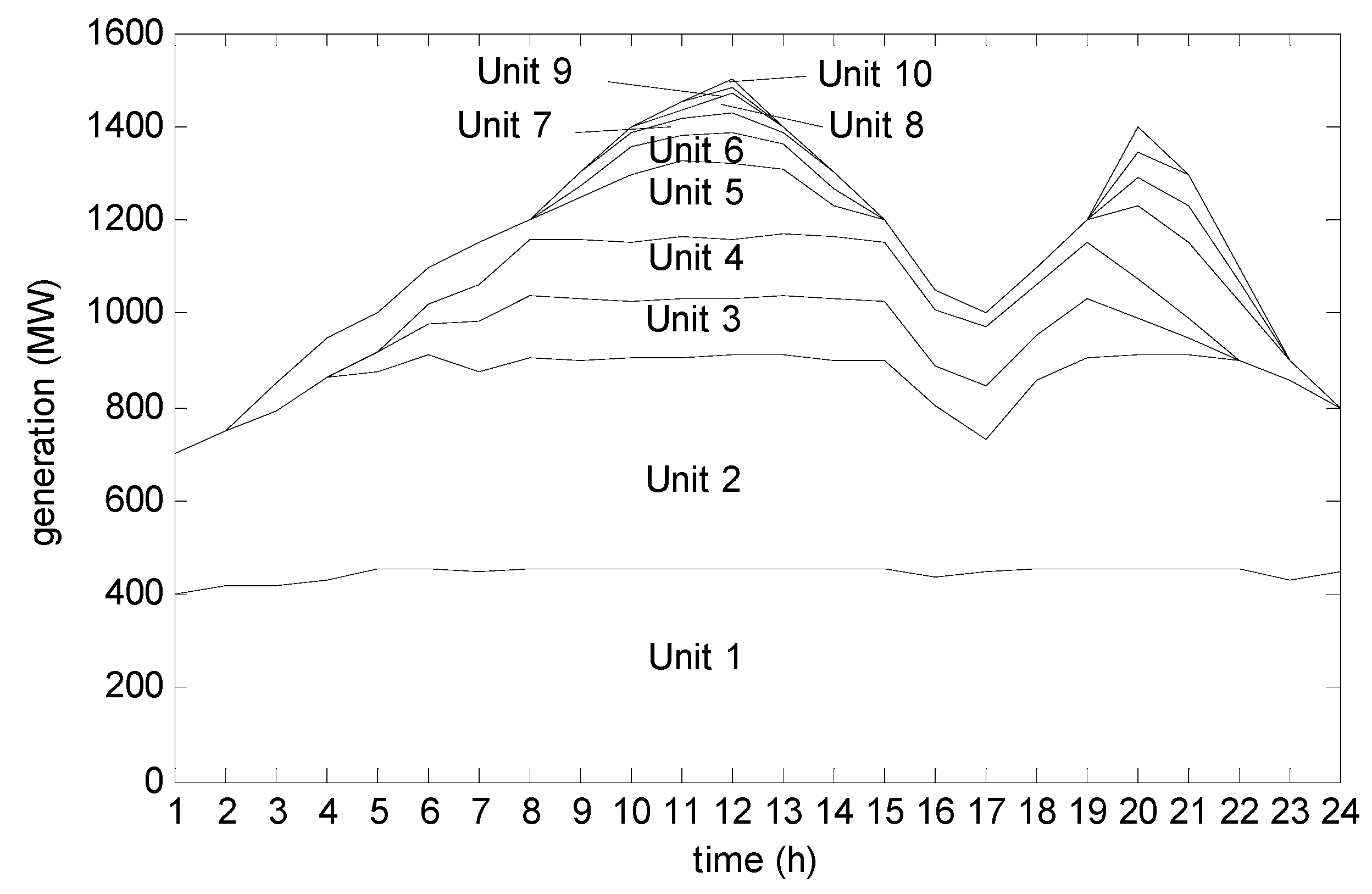
The generation of a 10–100-unit 24 h system is shown in Figure 4, where the area of each unit is the generation value.
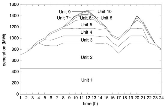
Figure 4.
Generation of the 10 units (not considering unit ramp rate constraint).
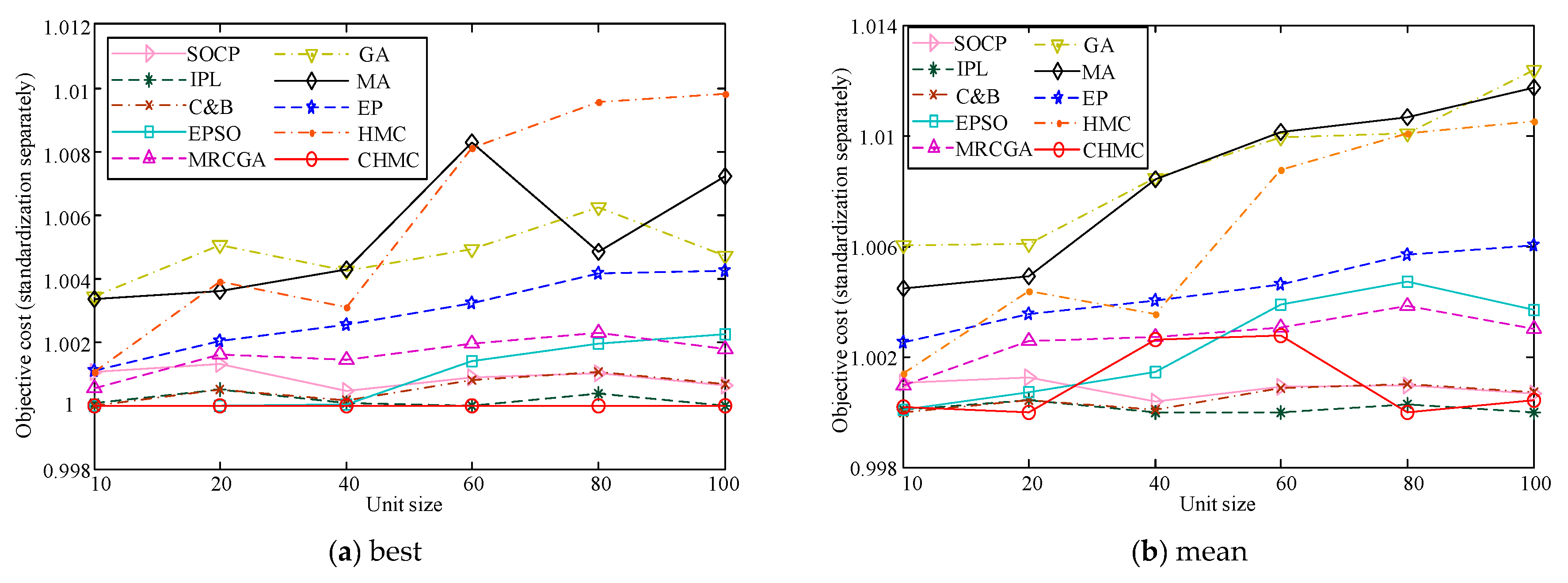
Comparison of the proposed CEHMC with six bioinspired optimization methods (EPSO, MRCGA, GA, MA, EP, HMC) and three mathematical optimization methods (SOCP, IPL, C&B) is shown in Table 3. To be more illustrative, the normalized comparison results of different algorithms are plotted in Figure 5. For the bioinspired optimization methods, the best and mean solutions of them are plotted as Figure 5a,b, respectively.
Table 3.
Comparison of different algorithms (not considering unit ramp rate constraint), unit: $.
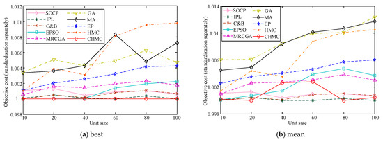
Figure 5.
Normalized comparison results of different algorithms (not considering unit ramp rate constraint).
From the best solutions, it can be seen that CEHMC has the best performance in all the seven intelligent methods. Compared with the three mathematical optimization methods, the best solutions of CEHMC are lightly larger than IPL (with the smallest objective cost) when unit size is 60 and 80. In other cases of unit size, CEHMC gets the best results. That means, the proposed CEHMC has stable optimization process when unit size increases. Comparing the results of CEHMC and HMC, the solution of CEHMC is much better than HMC. It is shown that the hybrition of cross-entropy and membrane computing theory can significantly improve the optima searching ability and optimization efficiency.
5.2. Simulation Results of UC Problem with Ramp Constraints
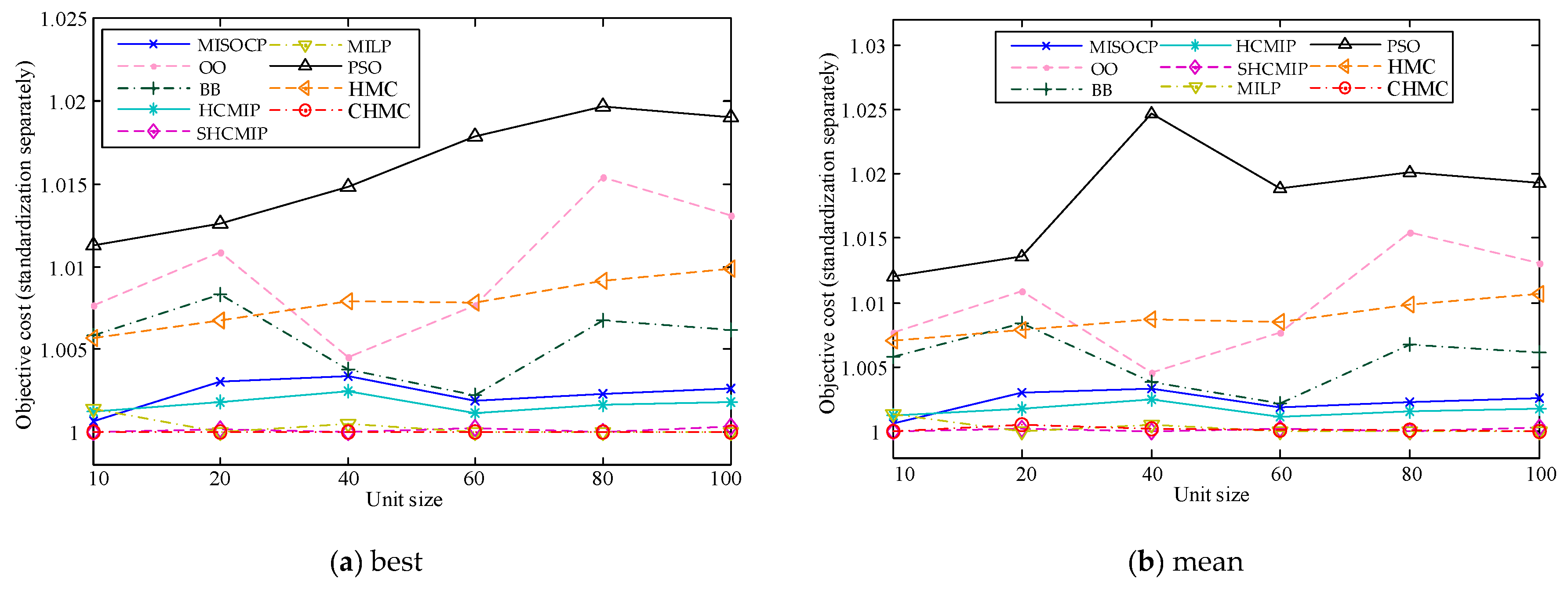
The generation of a 10-unit 24 h system is shown in Figure 6, where the area of each unit is the generation value. Comparison of the proposed CEHMC with two intelligent optimization methods (PSO, HMC) and six mathematical optimization methods (MISOCP, OO, BB, HCMIP, SHCMIP, MILP) is shown in Table 4. To be more illustrative, the normalized comparison results of different algorithms are also plotted in Figure 7. For PSO, HMC and CEHMC, the best solutions of them are plotted as Figure 7a,b, respectively.

Figure 6.
Generation of 10 units (considering unit ramp rate constraint).
Table 4.
Comparison of different algorithms (considering unit ramp rate constraint), unit: $.
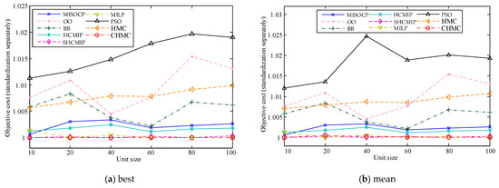
Figure 7.
Normalized comparison results of different algorithms (considering unit ramp rate constraint).
It is found that, with the unit size larger than 40, CEHMC has the best performance in all the nine optimization methods. In other cases of unit size, the best result of CEHMC is lightly larger than the optima of all the nine optimization algorithms. The introduction of cross-entropy theory greatly improves the optima searching ability, which makes the results of CEHMC generally much better than HMC.
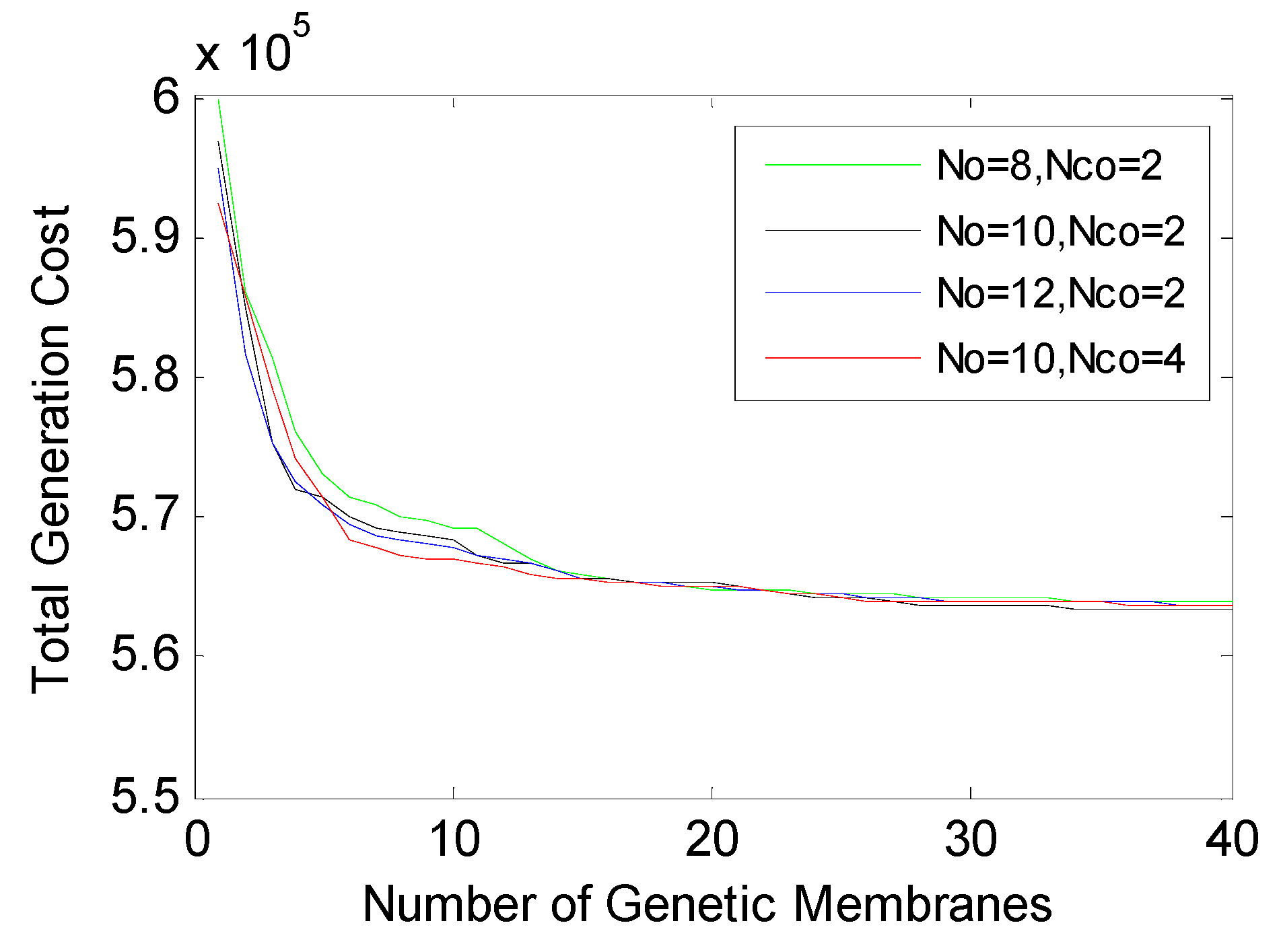
5.3. Influences of the Membrane Number to Convergence
For ease of explanation, the case of 10-unit without ramp constraints is taken as an example to analyze the influences of membrane number to approximation of optimal solution for the proposed CEHMC method.
5.3.1. GAPS
The effect of membrane number in GAPS on the objective value is simulated and illustrated in Figure 8. It is found that No and Nco may have little influence on the convergence with all those curves have similar shapes. Considering the computation cost and matching with other parameters, No is set as 10, and Nco is 10.
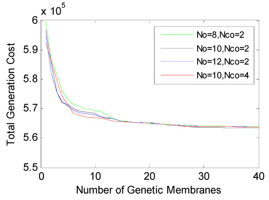
Figure 8.
Influence of membrane number to convergence (GAPS).
5.3.2. BMC
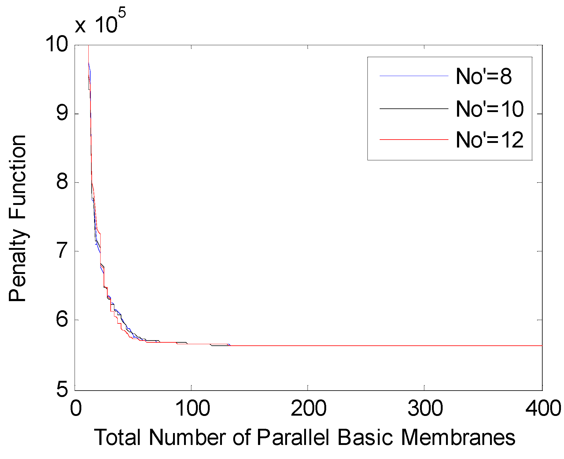
BMC is for the dynamic dispatching problem with continuous variables. The influence of membrane number to convergence for BMC is based on a certain unit start-stop plan. The number of membranes is the product of Nc′ and Nb′, which can also represent the iteration number. Figure 9 shows the penalty value curves changing with membrane number of BMC. It is found that when the abscissa is 100, the curve is almost gentle. Therefore, Nc′ is set as 10, and Nb′ is 10.

Figure 9.
Influence of membrane number to convergence (BMC).
5.4. Analysis of Calculation Efficiency
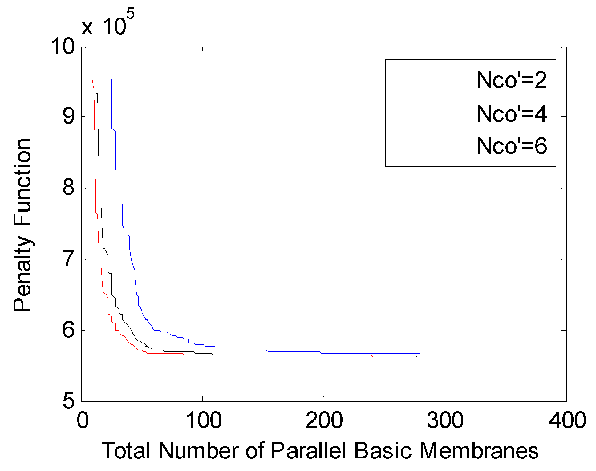
Figure 10 shows how Nco′ influences the approaching to the optimal solution. It is found that Nco′ have effect on convergence. When Nco′ is set 6, the convergence rate is fastest. when Nco′ is set 2, the convergence rate is the slowest. After comprehensive consideration, the value of Nco′ is set 4.
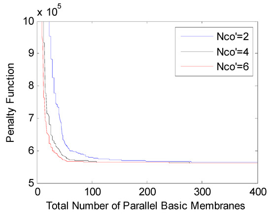
Figure 10.
The sensitivity of Nco′ to convergence (BMC).
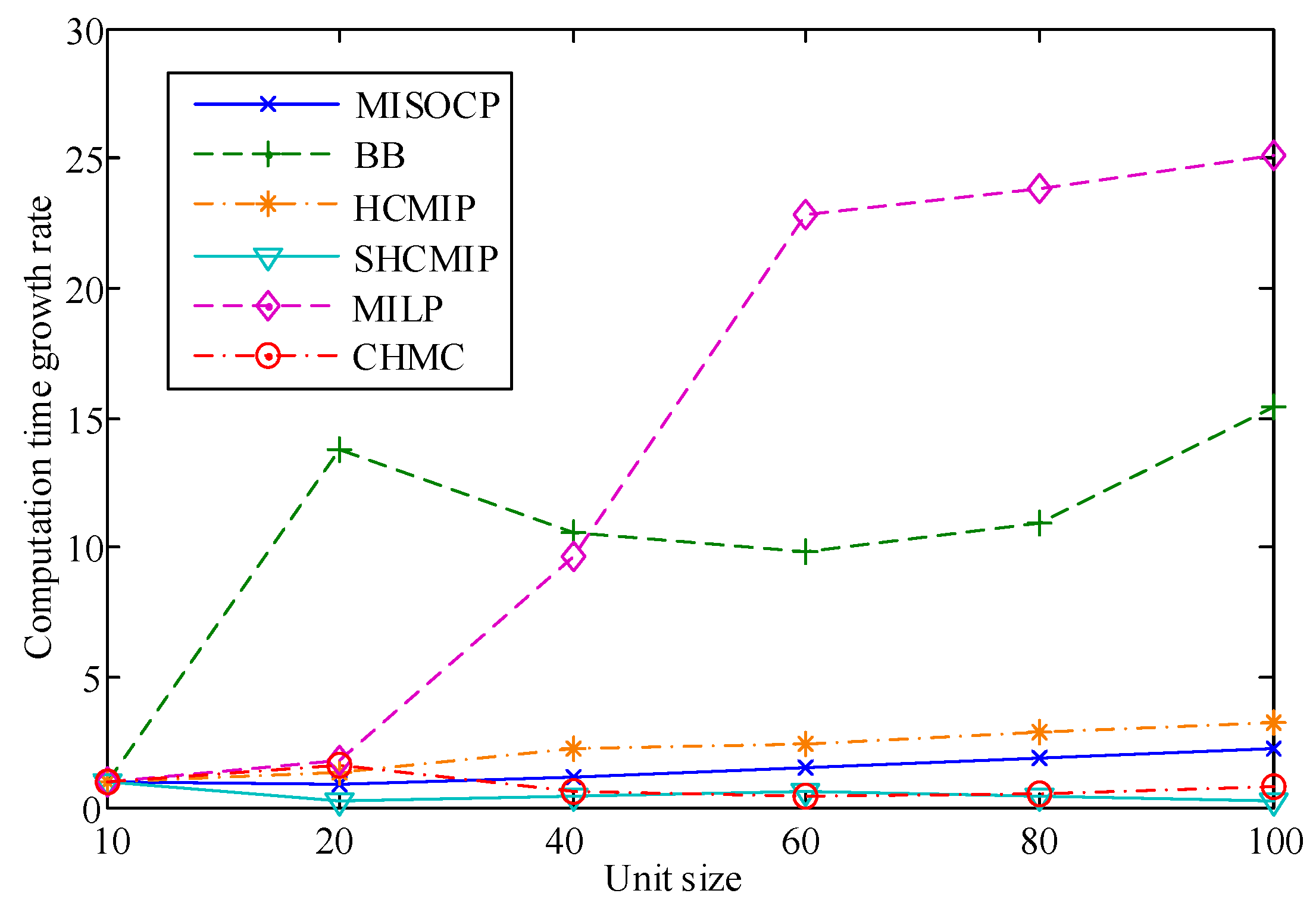
In order to verify the calculation efficiency of the proposed method, the calculation efficiency for the proposed CEHMC method and the other methods (in Table 4) are analysed and compared. The unit ramp rate constraints are considered. The computation time growth rate curves with the unit size increasing from 10 to 100 are illustrated in Figure 11. The computation time growth rate is based on the time consumed for the case of 10-unit.
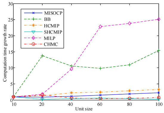
Figure 11.
Computation time growth rate curves (considering unit ramp rate constraint).
It can be seen that only SHCMIP has a little better calculation efficiency than the proposed CEHMC method as the unit size increases. The time growth rate of CEHMC is significantly lower than the other four methods (MISOCP, BB, HCMIP, MILP) for large-scale UC problems.
6. Conclusions
In this paper, a cross-entropy-based hybrid membrane computing method is proposed to solve the UC problem which is inspired by living cells and their organization in tissues and other higher order structures. In the proposed method, the genetic algorithm-based P system is applied for the unit start-stop plan with embedded generic rules, which can transmit the outer optima into the inner membranes. The biomimetic membrane computing method combined with the cross-entropy is proposed to solve the dynamic economic dispatch problem with strengthened searching ability, which is inspired by the important role of Golgi apparatus in living cells. The 10–100 unit systems for 24 h day-ahead dispatching simulation results showed that the UC problem could be solved by the proposed method with good efficiency and stability. In future research, network constraints will be considered, and the method will be further improved to optimize simulation results.
Author Contributions
Conceptualization, M.X.; methodology, Y.D.; software, Y.D. and P.C.; validation, W.W.; writing—original draft preparation, Y.D.; writing—review and editing, M.X.; supervision, M.X. and M.L.; funding acquisition, M.X.
Funding
The financial supports for this research, from Guangdong Natural Science Foundation Free Application Project (2018A0303130134), are gratefully acknowledged.
Conflicts of Interest
The authors declare no conflict of interest.
References
- Pandžić, H.; Dvorkin, Y.; Qiu, T.; Wang, Y.; Kirchen, D. Toward cost-efficient and reliable unit commitment under uncertainty. IEEE Trans. Power Syst. 2016, 31, 970–982. [Google Scholar] [CrossRef]
- Mohammad, J.F.; Mitch, C.; Shabbir, A.; Ahmed, S.; Grijalva, S. Large-scale decentralized unit commitment. Int. J. Electr. Power Energy Syst. 2015, 73, 97–106. [Google Scholar]
- Bai, Y.; Zhong, H.; Xia, Q.; Kang, C. A decomposition method for network-constrained unit commitment with AC power flow constraints. Energy 2015, 88, 595–603. [Google Scholar] [CrossRef]
- Quan, R.; Jian, J.; Yang, L. An improved priority list and neighborhood S. Arch method for unit commitment. Int. J. Electr. Power Energ. Syst. 2015, 67, 278–285. [Google Scholar] [CrossRef]
- Yuan, W.; Zhai, Q. Power-based transmission constrained unit commitment formulation with energy-based reserve. IET Gener. Trans. Distrib. 2017, 11, 409–418. [Google Scholar] [CrossRef]
- Zheng, H.; Jian, J.; Yang, L.; Quan, R. A deterministic method for the unit commitment problem in power systems. Comput. Oper. Res. 2016, 66, 241–247. [Google Scholar] [CrossRef]
- Nasri, A.; Kazempour, S.J.; Conejo, A.J.; Ghandhari, M. Network-constrained AC unit commitment under uncertainty: A benders decomposition approach. IEEE Trans. Power Syst. 2015, 31, 412–422. [Google Scholar] [CrossRef]
- GAMS Development Corporation. GAMS, the Solvers’ Manual, 2015. Available online: http://www.gams.com/solvers (accessed on 1 December 2018).
- Rouhi, F.; Effatnejad, R. Unit commitment in power system t by combination of dynamic programming (DP), genetic algorithm (GA) and particle swarm optimization (PSO). Indian J. Sci. Technol. 2015, 8, 134. [Google Scholar] [CrossRef]
- Magnússon, S.; Weeraddana, P.C.; Rabbat, M.G.; Fischione, C. On the convergence of alternating direction Lagrangian methods for nonconvex structured optimization problems. IEEE Trans. Control Netw. Syst. 2016, 3, 296–309. [Google Scholar] [CrossRef]
- Sun, L.; Zhang, Y.; Jiang, C. A matrix real-coded genetic algorithm to the unit commitment problem. Electr. Power Syst. Res. 2006, 76, 716–728. [Google Scholar] [CrossRef]
- Shukla, A.; Singh, S.N. Multi-objective unit commitment using search space-based crazy particle swarm optimisation and normal boundary intersection technique. IET Gener. Trans. Distrib. 2016, 10, 1222–1231. [Google Scholar] [CrossRef]
- Valenzuela, J.; Smith, A.E. A seeded memetic algorithm for large unit commitment problems. J. Heuristics 2002, 8, 173–195. [Google Scholar] [CrossRef]
- Wang, H.; Peng, H.; Shao, J.; Wang, T. A thresholding method based on P systems for image segmentation. ICIC Express Lett. 2012, 6, 221–227. [Google Scholar]
- Wang, X.; Zhang, G.; Zhao, J.; Rong, H.; Ipate, F.; Lufticaru, R. A modified membrane-inspired algorithm based on particle swarm optimization for mobile robot path planning. Int. J. Comput. Comm. Control 2015, 10, 732–745. [Google Scholar] [CrossRef]
- Xiao, J.H.; Zhang, X.Y.; Xu, J. A membrane evolutionary algorithm for DNA sequence design in DNA computing. Chin. Sci. Bull. 2012, 57, 698–706. [Google Scholar] [CrossRef]
- Zhao, J.; Wang, N. A bio-inspired algorithm based on membrane computing and its application to gasoline blending scheduling. Comput. Chem. Eng. 2011, 35, 272–283. [Google Scholar] [CrossRef]
- Zhang, G.X.; Cheng, J.X.; Gheorghe, M. A membrane-inspired approximate algorithm for traveling salesman problems. Rom. J. Inf. Sci. Technol. 2011, 14, 3–19. [Google Scholar]
- Leporati, A.; Pagani, D. A membrane algorithm for the min storage problem. In International Workshop on Membrane Computing; Springer: Berlin/Heidelberg, Germany, 2006; pp. 443–462. [Google Scholar]
- Pereira, S.; Ferreira, P.; Vaz, A.I.F. A simplified optimization model to short-term electricity planning. Energy 2015, 9, 2126–2135. [Google Scholar] [CrossRef]
- Păun, G. Computing with membranes. J. Comput. Syst. Sci. 2000, 61, 108–143. [Google Scholar] [CrossRef]
- Păun, A. On P Systems with Active Membranes. Unconventional Models of Computation; UMC’2K; Springer: London, UK, 2001; pp. 187–201. [Google Scholar]
- Rubinstein, R. The cross-entropy method for combinatorial and continuous optimization. Methodol. Comput. Appl. Probab. 1999, 1, 127–190. [Google Scholar] [CrossRef]
- Kroese, D.P.; Porotsky, S.; Rubinstein, R.Y. The cross-entropy method for continuous multi-extremal optimization. Methodol. Comput. Appl. Probab. 2006, 8, 383–407. [Google Scholar] [CrossRef]
- Quinn, A.; Kárný, M.; Guy, T.V. Fully probabilistic design of hierarchical Bayesian models. Inf. Sci. 2016, 369, 532–547. [Google Scholar] [CrossRef]
- Yang, Z.; Gao, K.; Fan, K.; Lai, Y. Sensational headline identification by normalized cross entropy-based metric. Comput. J. 2015, 58, 644–655. [Google Scholar] [CrossRef]
- Senjyu, T.; Shimabukuro, K.; Uezato, K.; Funabashi, T. A fast technique for unit commitment problem by extended priority list. IEEE Trans. Power Syst. 2003, 18, 882–888. [Google Scholar] [CrossRef]
- Guo, S.; Guan, X.; Zhai, Q. The necessary and sufficient conditions for determining feasible solutions to unit commitment problems with ramping constraints. IEEE Power Eng. Soc. Gen. Meet. 2005, 1, 344–349. [Google Scholar]
- Yuan, X.; Tian, H.; Zhang, S.; Ji, B.; Huo, Y. Second-order cone programming for solving unit commitment strategy of thermal generators. Energy Convers. Manag. 2013, 76, 20–25. [Google Scholar] [CrossRef]
- Roy, P.K. Solution of unit commitment problem using gravitational search algorithm. Int. J. Electric. Power Energy Syst. 2013, 53, 85–94. [Google Scholar] [CrossRef]
- Juste, K.A.; Kita, H.; Tanaka, E.; Hasegava, J. An evolutionary programming solution to the unit commitment problem. IEEE Trans. Power Syst. 1999, 14, 1452–1459. [Google Scholar] [CrossRef]
- Quan, R.; Hua, W.; Jian, J. Solution of large scale unit commitment by second-order cone programming. Proc. CSEE 2010, 30, 101–107. [Google Scholar]
- Xie, M.; Zhu, Y.; Wu, Y.; Yan, Y.; Liu, M. Application of ordinal optimization theory to solve large-scale unit commitment problem. Control Theory Appl. 2016, 33, 542–551. [Google Scholar]
- Yang, L.; Jian, J.; Han, D.; Zheng, H. A hyper-cube cone relaxation model and solution for unit commitment. Trans. China Electrotech. Soc. 2013, 28, 252–261. [Google Scholar]
- Yang, L.; Jian, J.; Zheng, H.; Dan, D. A sub hyper-cube tight mixed integer programming extended cutting plane method for unit commitment. Proc. CSEE 2013, 33, 99–108. [Google Scholar]
- Liu, S.; Jian, J. Research on unit commitment considering emission trading. Power Syst. Technol. 2013, 3, 3558–3563. [Google Scholar]
© 2019 by the authors. Licensee MDPI, Basel, Switzerland. This article is an open access article distributed under the terms and conditions of the Creative Commons Attribution (CC BY) license (http://creativecommons.org/licenses/by/4.0/).