Article

Optimal Distribution Grid Operation Using DLMP-Based Pricing for Electric Vehicle Charging Infrastructure in a Smart City

1
GECAD—Knowledge Engineering and Decision Support Research Center—Polytechnic of Porto (IPP), R. Dr. António Bernardino de Almeida, 431, 4200-072 Porto, Portugal
2
University of Salamanca, 37008 Salamanca, Spain
3
Osaka Institute of Technology, 5 Chome-16-1 Omiya, Asahi Ward, Osaka 535-8585, Japan
4
University of Technology Malaysia, Pusat Pentadbiran Universiti Teknologi Malaysia, 81310 Skudai, Johor, Malaysia
*
Author to whom correspondence should be addressed.
Energies 2019, 12(4), 686; https://doi.org/10.3390/en12040686
Submission received: 22 January 2019 / Revised: 7 February 2019 / Accepted: 14 February 2019 / Published: 20 February 2019
(This article belongs to the Special Issue Intelligent Transportation Systems for Electric Vehicles)

Abstract

:
The use of electric vehicles (EVs) is growing in popularity each year, and as a result, considerable demand increase is expected in the distribution network (DN). Additionally, the uncertainty of EV user behavior is high, making it urgent to understand its impact on the network. Thus, this paper proposes an EV user behavior simulator, which operates in conjunction with an innovative smart distribution locational marginal pricing based on operation/reconfiguration, for the purpose of understanding the impact of the dynamic energy pricing on both sides: the grid and the user. The main goal, besides the distribution system operator (DSO) expenditure minimization, is to understand how and to what extent dynamic pricing of energy for EV charging can positively affect the operation of the smart grid and the EV charging cost. A smart city with a 13-bus DN and a high penetration of distributed energy resources is used to demonstrate the application of the proposed models. The results demonstrate that dynamic energy pricing for EV charging is an efficient approach that increases monetary savings considerably for both the DSO and EV users.

1. Introduction

The efforts to minimize the carbon footprint using a large-scale integration of renewable energy sources (RES), such as wind and solar energy, have led to innovative developments in power distribution systems around the world. Moreover, a new agreement in the European Union (EU) aims to achieve 27% penetration of RES by 2030 [1], as one-third of EU countries have already achieved the 2020 target [2].
Currently, many people move to cities in search of a better quality of life, and this contributes to the continuous expansion of urban areas, which play a major role in modern economies. However, the urban population is responsible for most greenhouse gas emissions, and the United Nations estimates that the urban population will reach 70% of the world’s total population by 2050 [3]. Consequently, it is necessary to make intelligent use of resources in urban environments, contributing to the development of smart cities [3]. The energy infrastructure of a smart city (SC), the so-called smart grid (SG), is one of the most important urban infrastructures that allows creating a sustainable city [4]. To this end, it is necessary to modernize grid functionalities through the implementation of innovative technologies, concretely, SG-enabling technologies for information and communication, sensing and measurement, automation, control, renewable generation integration, and storage [5,6].
One of the primary sources of CO 2 emissions is transportation [7,8]. Several authors have been analyzing the benefit of changing from traditional transportation (internal combustion engines) to EVs, in minimizing the transport sector’s greenhouse gas emissions. It is widely acknowledged that the shift from internal combustion engines to EVs has many environmental and economic advantages. However, the increasing number of EVs makes it necessary to develop new infrastructure continually for EV charging, and this, in turn, leads to a growing energy demand [9,10]. These charging infrastructures are going to burden the distribution power grid [11,12,13], namely the high charging loads of fast EV charging stations. Furthermore, some distribution network operating parameters are going to degrade. Several published works describe the negative impacts of EV charging on the following distribution network parameters:
Thus, a high EV penetration level may congest the distribution network. Congestion problems can be managed by the DSO, who reinforces the system through long-term planning or market-based congestion control methods [31]. The transmission systems concept of locational marginal pricing (LMP) can be extended to distribution systems [32]; it uses distributed generation (DG) units to handle congestion in distribution networks [33,34,35,36,37] and is usually referred to as distribution locational marginal pricing (DLMP). To deal with EV demand congestion in DN, the work in [38] proposed a step-wise congestion management whereby the DSO predicts congestion for the next day and publishes day-ahead tariff prior to the clearing of the day-ahead market, while [39] solved the social welfare optimization of the distribution system considering EV aggregators as price takers in the local DSO market and demand price elasticity. Liu et al. presented in [40] a market-based mechanism taken from the DLMP concept to alleviate possible distribution system congestion caused by the integration of EVs and heat pumps. Similarly, the authors in [41] proposed a DLMP based on quadratic programming to deal with the congestion in distribution networks with a high penetration of EVs and heat pumps.
As is known, the EVs are additional electric loads and represent mobile energy storage, usually with long resting times. Several mathematical models presented in [42,43,44,45,46,47] also studied the impact of EV charging in the distribution networks. The works in [48,49,50,51,52,53] assessed several possibilities for demand-side management, as well as better coordination of charging processes through price incentives that mitigate the impact of EV charging during peak-loads. The works in [54,55,56,57,58] proposed an increase in EV charging flexibility, contributing to increased utilization of the highly-variable renewable energy. Moreover, one of the main challenges in facilitating integrated EV charging in the distribution network is EV user behavior modeling and prediction [59]. Optimal control for allocating EV charging time and energy optimally has been proposed by Gan et al. [60]. However, the model requires that users frequently provide the charging schedule, requiring significant effort on the part of the customer. The algorithms developed in [61] used an EV random user behavior model with renewable generation for EV scheduling, while [62] provided a smart charging strategy according to time-of-use price from the day-ahead forecast. The authors in [63,64,65,66] examined EV users’ charging behavior and measured psychological variables, an analysis that can help develop new charging strategies.
SCs feature an active power architecture with a high penetration of distributed energy resources (DER), challenging the conventional control and operation framework designed for passive distribution networks. In this context, the loads can be supplied not only by traditional generation units at the upstream power systems, but also by the DER [67]. Thus, a distribution network reconfiguration (DNR) will be a very important and significant strategy for the DSO. DNR is a process that changes the network topology using the remote switches such that all the network constraints are considered. Traditionally, the DNR is associated with system power loss minimization [68,69]; however, in the SG, context the DNR must not only meet the classic objectives, such as power loss, minimization of power not supplied, and improvement of the voltage profile, but also the problems related to the high DER integration and the intelligent reconfiguration related to the SG paradigm [70,71,72]. Several works considering mathematical [73,74,75], heuristics and metaheuristics [76,77], and hybrid models [78,79] were developed to deal with DNR and DER penetration.
The above-cited literature has not addressed distribution network operation and reconfiguration simultaneously in an SG context; neither have they considered the high penetration of DER and EV user behavior, nor dynamic EV charging price through DLMPs. Thus, to the best of the authors’ knowledge, the answer to the question “Can dynamic EV charging price, have a positive impact on both the operation of the smart distribution network and on EV user behavior?” has not yet been answered. To answer this question, the authors combined an EV behavior simulator with a proposed innovative smart DLMP-based distribution network operation/reconfiguration. This kind of problem is classified as mixed-integer nonlinear programming (MINLP) due to its nonlinear features requiring significant computer resources. To deal with the issue of computational burden and at the same time improve the tractability of the model, the Benders decomposition method is used. This method uses duality theory [80,81] in linear and nonlinear mathematical programming, and it deals with complex problems by splitting them into subproblems. The main goal is to minimize all the DSO expenditures. To this end, the proposed methodology seeks the following:
  • Minimize power loss;
  • Minimize power not supplied;
  • Minimize line congestion;
  • Minimize the power generation curtailment;
  • Minimize the power from external suppliers;
  • Distribution network radial topology.
Considering the research gaps in previous works, this paper presents the following major contributions:
  • The use of an EV user behavior simulator. This simulator is used to simulate the EV user behavior aspects, such as: stochastic EV user aspects, importance of EV charging price, importance of comfort, choosing slow or fast charge, and the user sensibility of the the state of the battery;
  • Present a distribution network operation/reconfiguration optimization problem in an SG context with high DER penetration concerning the behavior aspects of the EV users and the dynamic EV charging price considering DLMPs using the Benders decomposition method;
  • Analyze how and to what extent dynamic EV charging prices contribute positively to smart distribution network operation;
  • Understand how and to what extent dynamic EV charging prices can contribute to a positive impact on the electric vehicles’ charging cost.
To demonstrate the application of the proposed methodology, the BISITE (https://bisite.usal.es/en) laboratory’s SC mockup model has been used with a 13-bus distribution network and high DER penetration. This paper is organized as follows: after this Introduction, Section 2 presents the proposed methodology and the details of the DLMP-based network operation, as well as the simulation of urban mobility. To verify the performance of the proposed methodology, a case study has been conducted and described in Section 3. The results and its discussion are presented in Section 4. Finally, Section 5 presents the most relevant conclusions.

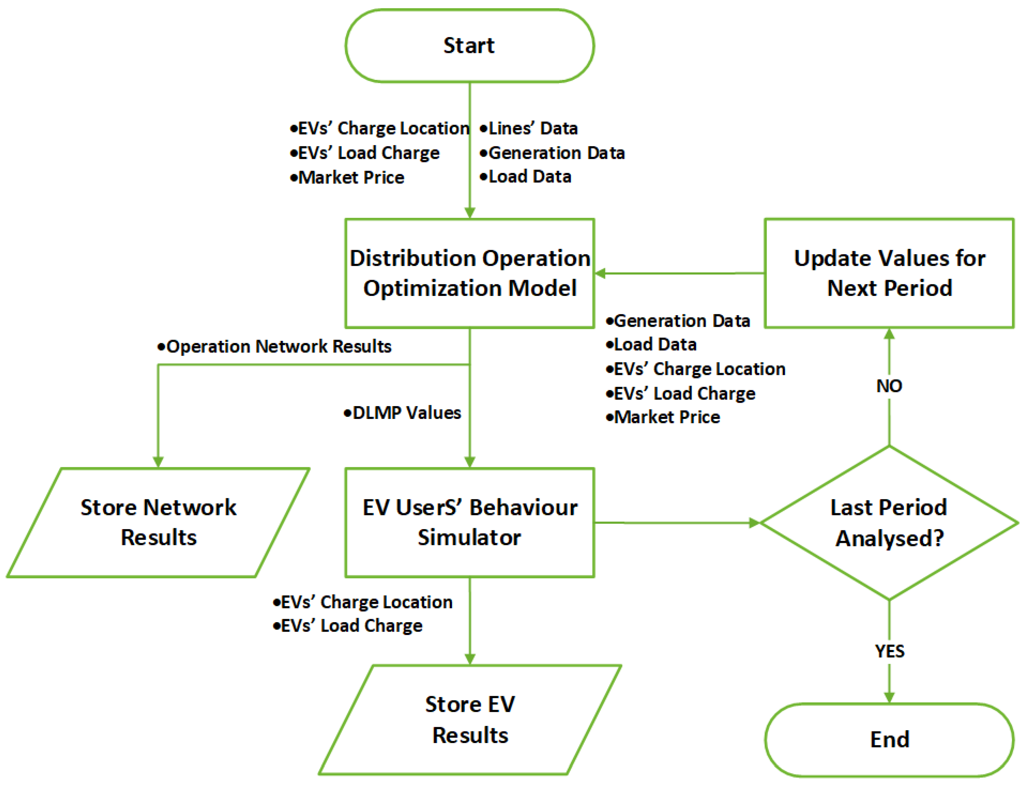
2. Proposed Methodology

This section presents a detailed description of the adopted methodology (depicted in the Figure 1). Section 2.1 provides information about the EV user behavior simulator, while Section 2.2 describes the DLMP-based network operation model using the Benders decomposition method.

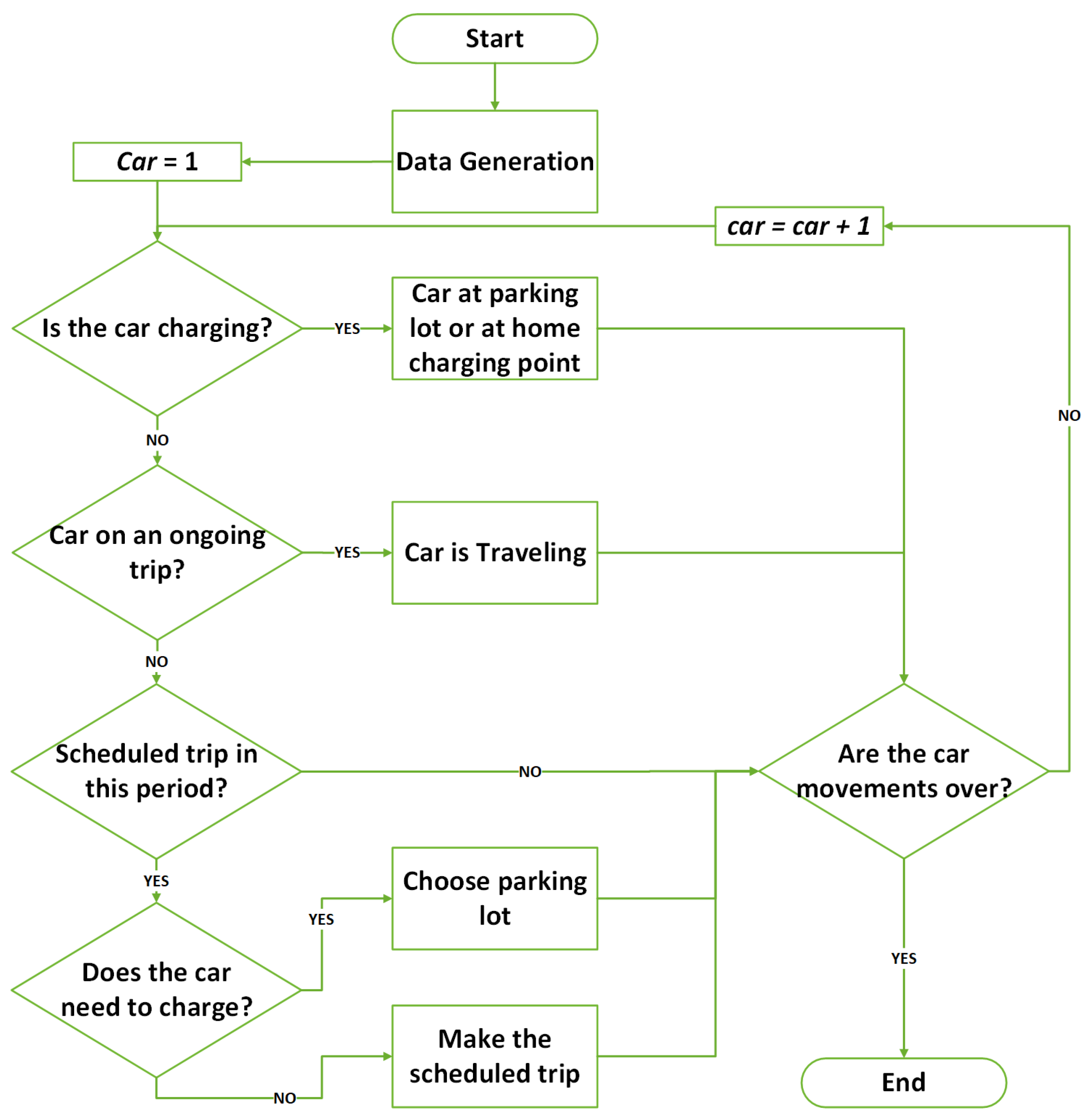
2.1. Simulator of Urban Mobility

The simulator module is able to generate a realistic population, considering the size of the network and the parking lots. It has several global and behavior-related parameters (user profiles) discussed later in this section. Figure 2 shows the flowchart of the simulator. After receiving the necessary information from the optimization model, i.e., the DLMP price in each bus of the network, the simulator loops for every individual car to perform the next period’s decision (i.e., 15 min). There are only two possible types of decisions: the decision to travel to a destination or a charging decision. Indeed, some trips take more than 15 min, so the car can just keep traveling for a certain number of periods. According to each user preference and behavior, decisions will be affected by the price and distance to the parking lot. Since, in a realistic scenario, some prefer extra comfort even if they pay more, e.g., choosing a fast charge or closer parking lot, the simulator allows defining this range of preferences for each car. These preferences will affect the efficacy of the dynamic EV charging prices, since individual behaviors may neglect lower prices. Nevertheless, our case study provides a different range of behavioral aspects to provide an accurate research outcome in this work.
To determine the dynamic EV charging price, the simulator uses the following Equation (1):
D E P = ( D L M P + T a r i f f M V + A C N R ) · P L G · V A T
where:
  • DEP: Dynamic EV charging price for each period (€/kWh)
  • DLMP: Distribution locational marginal pricing (€/kWh)
  • TariffMV: Energy tariff price for each period (in the Case Study Section, the reader can find the energy tariff price for each considered period) (€/kWh)
  • PLG: Additional profit margin of the parking owner
  • VAT: Value-added tax
  • ACNR: Additional cost related to the fixed term of network price rate to be charged to the customer (€/kWh) and given by (2):
    A C N R = 0.397 · C P 720 O P R
The contracted power cost is 0.397 €/kW/month, to be paid to the DSO monthly (www.erse.pt); the CP is the charging power of the parking lot; 720 are the hours per month; and OPR is the parking occupation rate. With the ACNR term added to Equation (1), the contracted power cost is transferred to the final consumer. Moreover, it is important to note that OPR is introduced to approximate the real occupation rate of each parking lot and thus affects the ACNR cost, which decreases for each customer as the OPR rate increases.
The global parameters of the simulator are described in Table 1. These are permanent parameters in the simulation; however, their values can be modified according to the needs of each study. Since car travel is simulated using simplified mathematics for vehicle movement, parameter cdist represents the penalty on a given distance between two points, e.g., Origin A and Destination B, that the vehicle has to travel (trips). Ideally, the minimum distance to reach Destination B (e.g., work) would be the Euclidean distance; however, in a real-world scenario, the road network is not optimal in this sense. Parameter sf can be used to easily change the scale of the map and increase or decrease distances regarding a reference scenario. This allows easily studying the effects on the travel times and charging needs when the urban distance is varied. Parameter hcpower enables setting the amount of charge power available when users decide to charge at home. Parameter chargineff is the charging efficiency considered for the energy transactions with the electrical grid.
Table 2 describes the parameters related to the user profile, namely regarding the initial location of the car when the simulation begins and its location in subsequent steps. Each car in the simulation replicates the parameters depicted in this table. Among the defined parameters, the weights of w1, w2, and ti are significant. The weights correspond to the importance attributed to distance and price, respectively, while ti is used to prioritize trips, for instance going to work cannot be postponed. The weights allow the simulator to compute the behavioral score formula and in this way to decide where to charge the vehicle if needed. For users that give more preference to price while driving long distances in the quest for parking lots with lower charging prices, these prices are dynamic in time and space depending on the DLMP status of the grid. Users with hc = 0 cannot charge at home, but can charge at parking lots (street charging).

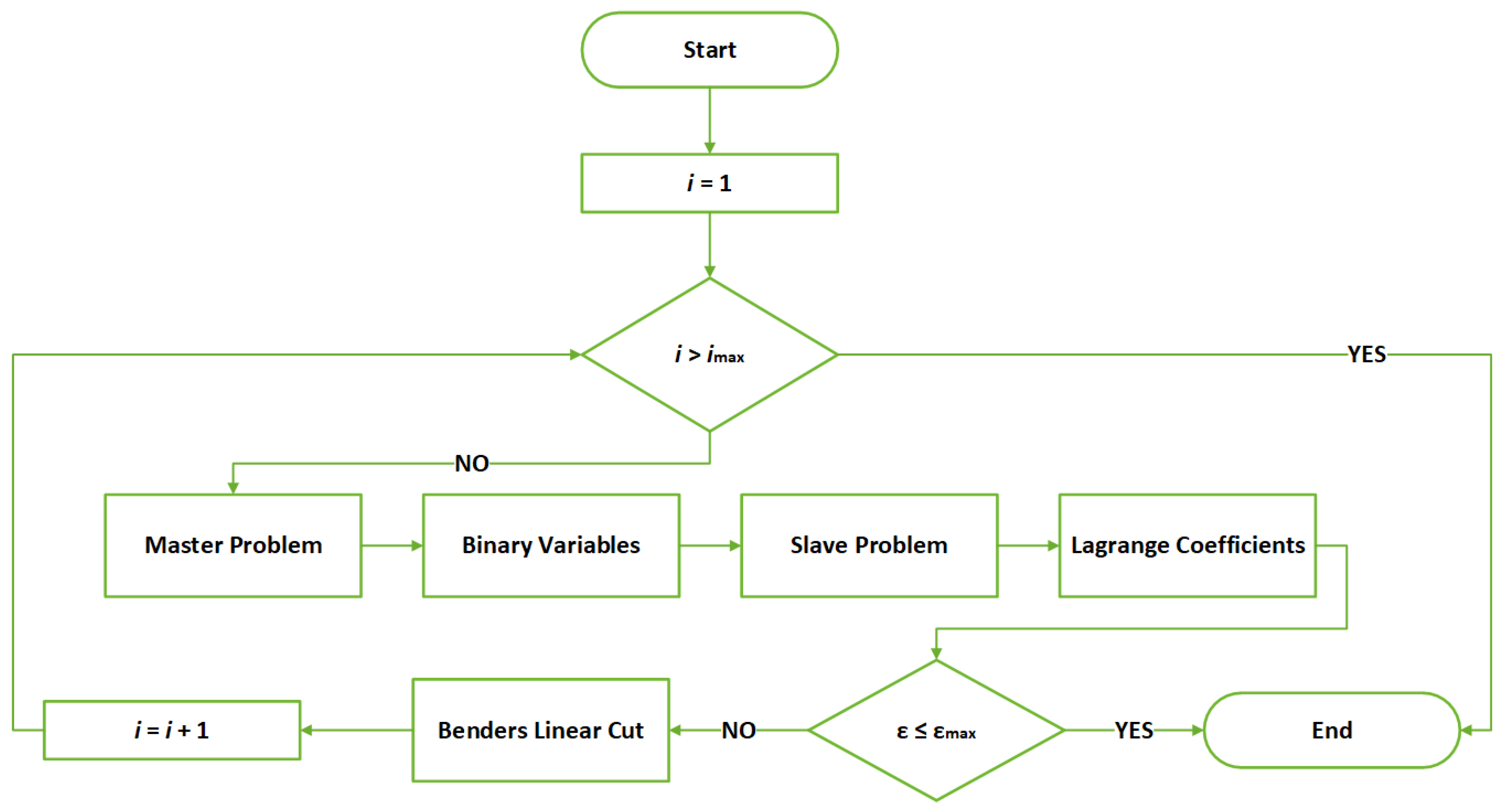
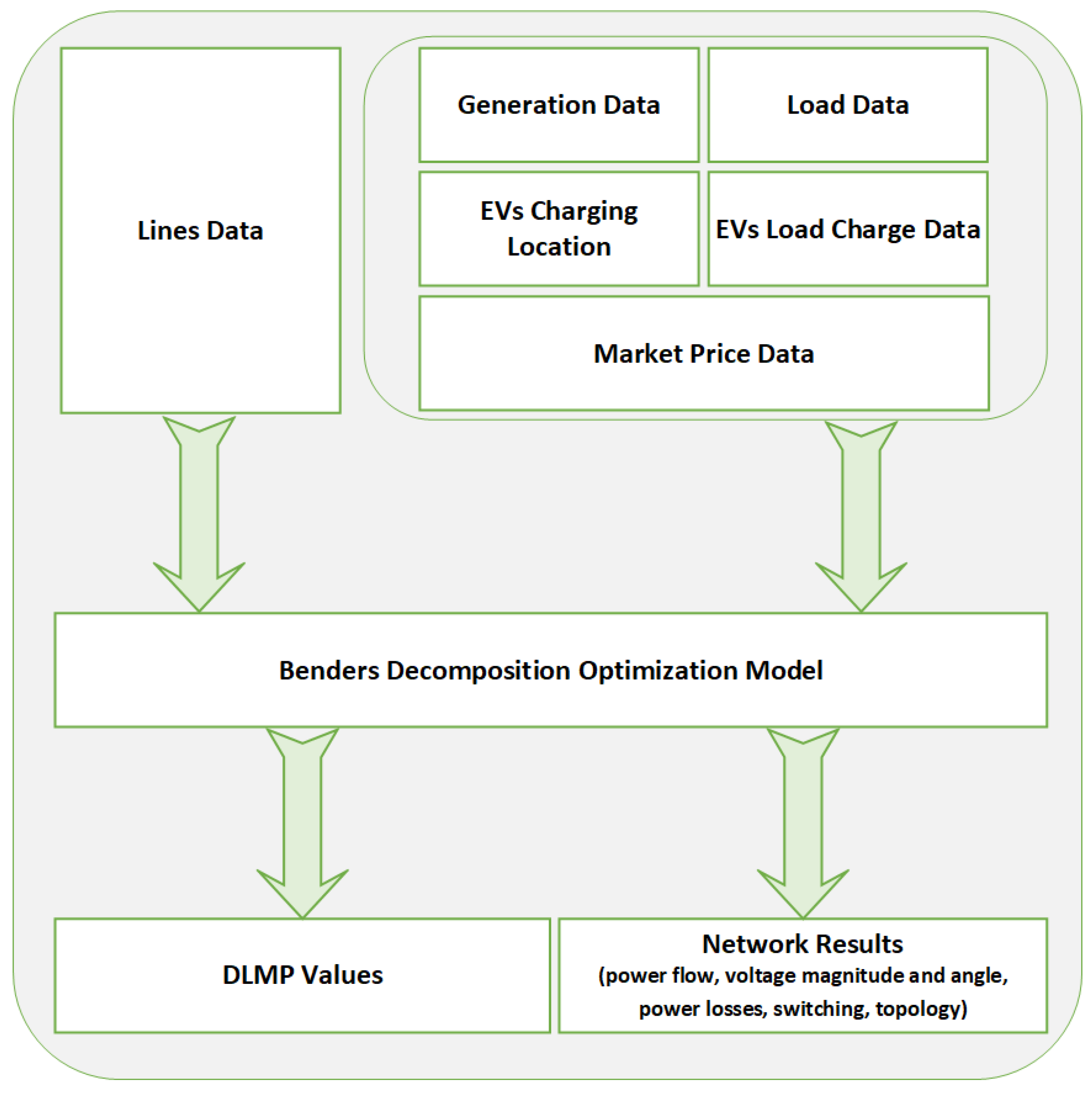
2.2. DLMP-Based Network Operation

DLMP has been studied to provide electricity players with the effective economic signals for optimizing their assets. It is known that the resistance of the distribution network lines is higher than that of transmission lines. Thus, the distribution system losses can be considered one of the main factors that affect the DLMP.
Bus voltage regulation is a critical issue, especially with DER proliferation, that is faced by the DSO. Therefore, the DLMP could reflect the voltage impact on the distribution system’s economical operation.
In the proposed methodology, DLMP is defined through Lagrangian multipliers of the corresponding constraints (power balance) of the optimization problem, whose goal is to minimize the DSO expenditures.
The distribution network operation and reconfiguration problem in an SG context with high DER penetration concerning the behavior aspects of the EV users and dynamic EV charging price considering DLMPs is classified as MINLP due to the nonlinearity features. To solve complex problems like this, the Benders decomposition is an adequate technique [80,81]. This technique was presented in 1962 by Jacobus Franciscus Benders to solve mixed integer problems [82]. This method is based on the principle that the main problem can be decomposed into sub-problems. The Benders decomposition technique uses duality theory in linear and nonlinear mathematical programming to split a problem whose resolution is difficult into sub-problems [80]. These sub-problems consider specific variables that are solved iteratively until the optimal solution is reached [83].
The problem can be divided into subproblems (a master problem and one or more slave problems). The master subproblem is usually a linear or mixed integer problem including fewer technical constraints. On the other hand, slave subproblems are linear or nonlinear and attempt to validate if the solution of the master problem is technically feasible or not. At this level, the network’s technical constraints are considered. A flowchart of the Benders decomposition technique used in this proposed research work is presented in Figure 3, and the diagram of the DLMP-based distribution network operation/reconfiguration model is presented in Figure 4. In Section 2.2.1 and Section 2.2.2, the explanation of the Benders decomposition procedure is discussed.
This work deals with a non-convex and non-linear slave subproblem (namely in the power flow equations) in which the zero-duality gap is not guaranteed. Thus, the Benders decomposition technique applied in this research work could not converge to the optimal solution. However, most of the science and engineering mathematical problems are non-convex with a very small duality gap in most of the cases [83]. Moreover, the convexity is a solid mathematical assumption, and the convexity is not necessarily restrictive from the practical viewpoint, as many science and engineering problems in the region where the solution of the interest is located are convex; in other words, where the solution is meaningful from the viewpoint of the science and engineering [83].

2.2.1. Master Problem

The master subproblem goal consists of finding the network topology configuration for each considered period by opening/closing tie-switches (using binary variables {0,1}) to:
  • Minimize the power losses’ cost;
  • Minimize the power not supplied cost;
  • Minimize the lines’ congestion cost;
  • Minimize the power generation curtailment cost;
  • Minimize the power from external suppliers’ cost.
At this level, every binary variables must be included in the optimization problem. The master subproblem objective function minimizes the operation cost (MOC) and can be formulated as (3):
M O C = i Ω B j Ω B C o n g M ( i , j ) 2 + C o n g M ( i , j ) · C o s t C o n g + i Ω B S b E x t S u p ( i ) · p r i c e M k + i Ω L b P N S M ( i ) · C o s t P N S + i Ω B j Ω B r ( i , j ) · F l o w M ( i , j ) 2 · C o s t L o s s + i Ω D G n d P P G C M ( i ) · P P G C C o s t + ω *
In the case of infeasibility, one variable is added to the master problem ( ω * ), which is called linear Benders’ cuts. In ideal circumstances, the value for this variable is zero, which means that the network topology along with its components fulfills every technical constraint. Otherwise, the value presented in this variable represents the minimal value cost change of the master solution.
The master subproblem (3) is subjected to constraints (4)–(25).
Network constraints
Power balance: First Kirchhoff law
Constraint (4) guarantees the power balance in each distribution network bus.
i Ω D G n d p D G ( i ) p P G C M ( i ) + i Ω B S b E x t S u p ( i ) i Ω L b p L o a d ( i ) P N S M ( i ) i Ω V b E V P ( i ) + i Ω E b S T d c h M ( i ) S T c h M ( i ) + i Ω B F l o w M ( i , j ) F l o w M ( j , i ) = 0 j Ω B
Maximum admissible line flow
The maximum power flowing in each line of the network is guaranteed by (5).
0 F l o w M ( i , j ) F l o w ( i , j ) max · X ( i , j ) s t a t X s t a t 0 , 1 , ( i , j ) Ω l
Unidirectionality of power flow
Constraint (6) guarantees unidirectionality between buses i and j.
X ( i , j ) s t a t + X ( j , i ) s t a t 1 X s t a t 0 , 1 , ( i , j ) Ω l
Radial topology
To ensure the radial topology, Constraint (7) is applied. This constraint imposes that only one line can enter in each bus.
j Ω j b X ( i , j ) s t a t = 1 X s t a t 0 , 1 , i Ω B
Avoid island creation
To avoid DG isolation from the substation, the constraints (8)–(11) are used. A fictitious flow ( d ( i , j ) ) is created with a fictitious load of each DG ( D ( g ) ) to be fed to the substation. If the island is permitted, the operator can omit these constraints.
i Ω B j Ω B d ( i , j ) i Ω B j Ω B d ( j , i ) D ( g ) = 0 g Ω D G
D ( g ) = 1 g Ω D G
D ( g ) = 0 g Ω D G Ω B S
d ( i , j ) n D G · X ( i , j ) s t a t ( i , j ) Ω l
Supplier constraint
Maximum and minimum limits for power supplier
The power is constrained by the maximum and minimum capacity that can be supplied (12).
E x t S u p M i n L i m i t ( b s ) E x t S u p ( b s ) E x t S u p M a x L i m i t ( b s ) b s Ω B S
Curtailment constraints
Power generation curtailment
The power generation curtailment is verified when the excess generation of the generator g occurs. This variable is lower or equal to the power generation of the g generator (13).
0 p P G C M ( g ) p D G ( g ) g Ω D G n d
Power not supplied
Constraint (14) guarantees that the power not supplied variable must be lower than or equal to the load demand.
0 P N S M ( l o ) p L o a d ( l o ) l o Ω L b
Lines’ congestion
Lines’ power congestion
The power congestion in each line is constrained by Equation (15). In this work, we assume that the congestion occurs when the power flow F l o w ( i , j ) is greater than or equal to a factor value ( C o n g M i n ) multiplied by the maximum power line capacity ( F l o w ( i , j ) m a x ). The factor value is a constant value between zero and one. In fact, this value represents the percentage of the line capacity that is being used. Equation C o n g ( i , j ) 0 is used to ensure a positive or a zero value for C o n g ( i , j ) .
C o n g M ( i , j ) F l o w M ( i , j ) C o n g M i n · F l o w ( i , j ) m a x ( i , j ) Ω l C o n g ( i , j ) 0
Energy storage systems (ESS) constraints
Discharge limit for the energy storage systems
The maximum discharge limit of each ESS is represented by the constraint (16).
S T d c h M ( e ) S T d c h R ( e ) · S T d M ( e ) s t a t e Ω E b , S T d M s t a t 0 , 1 , S T d c h M 0
Charge limit for the energy storage systems
The maximum charge limit for each ESS is represented by the constraint (17).
S T c h M ( e ) S T c h R ( e ) · S T c M ( e ) s t a t e Ω E b , S T c M s t a t 0 , 1 , S T c h M 0
Discharge level limit considering the state of the energy storage system
The maximum discharge limit considering energy storage systems’ capacity constraint for each ESS is given by (18). The Δ t is represented in units of hours.
S T d c h M ( e ) · 1 d e f ( e ) S T d M ( e ) s t a t · S T s t o M ( e ) · 1 Δ t e Ω E b , S T d M s t a t 0 , 1 , S T d c h M 0
Charge level limit considering energy storage systems’ capacity
The maximum charge limit considering energy storage systems’ capacity constraint for each ESS is given by (19). The Δ t is represented in units of hours.
S T s t o M ( e ) + S T c h M ( e ) · c e f ( e ) · Δ t S T c M ( e ) s t a t · S T c a p ( e ) e Ω E b , S T c M s t a t 0 , 1 , S T c h M 0
State of charge of the energy storage systems
The state of charge of each ESS is given by (20). The Δ t is represented in units of hours.
S T s t o M ( e ) Δ t · S T c h M ( e ) · c e f ( e ) + Δ t · S T d c h M ( e ) · 1 d e f ( e ) = S T s t o M ( e ) t 1 e Ω E b , S T c h M 0 , S T d c h M 0
Maximum ESS capacity limit
The maximum capacity limit of each ESS is represented by (21).
S T s t o M ( e ) S T c a p ( e )
Minimum ESS capacity limit
The minimum capacity limit of each ESS is represented by (22).
S T s t o M ( e ) S T s t o M ( e ) min
Charging and discharging status
The charging and discharging status of the ESSs are represented by S T c M ( e ) s t a t and S T d M ( e ) s t a t , respectively. Charging and discharging cannot occur simultaneously (23).
S T c M ( e ) s t a t + S T d M ( e ) s t a t 1
where S T c M ( e ) s t a t is a binary variable. ESS are able to charge at any moment.
S T d M ( e ) s t a t is a variable that assumes zero or one according to the study period market price value and is given by (24).
S T d M ( e ) s t a t = 1 p r i c e M k p r i c e min M k S T d M ( e ) s t a t = 0 p r i c e M k p r i c e min M k
Linear Benders’ cut
To support the decomposition technique, a linear cuts constraint (25) is used. This constraint represents feasibility cuts in the problem. These cuts are updated in each iteration applying new constraints to the problem. The linear cuts establish the link between the master subproblem and the slave subproblem. To better understand, let us imagine the existence of a cut. Thus, the master subproblem receives and considers the infeasibility data costs of the previous iteration ω * and the sensitivities λ ( i , j ) m 1 and μ ( i ) m 1 . Those sensitivities are linked to the subproblem master decision in the previous iteration X ( i , j ) s t a t m 1 and S T c M ( i ) s t a t m 1 already known. To make a new decision, the master subproblem is fed these new data.
ω * Z u p m 1 + i Ω B j Ω B j i λ ( i , j ) m 1 · X ( i , j ) s t a t m X ( i , j ) s t a t m 1 + i Ω B S b μ ( i ) m 1 · S T c M ( i ) s t a t m S T c M ( i ) s t a t m 1
where index m represents the current iteration and m-1 represents the previous iteration.

2.2.2. Slave Problem
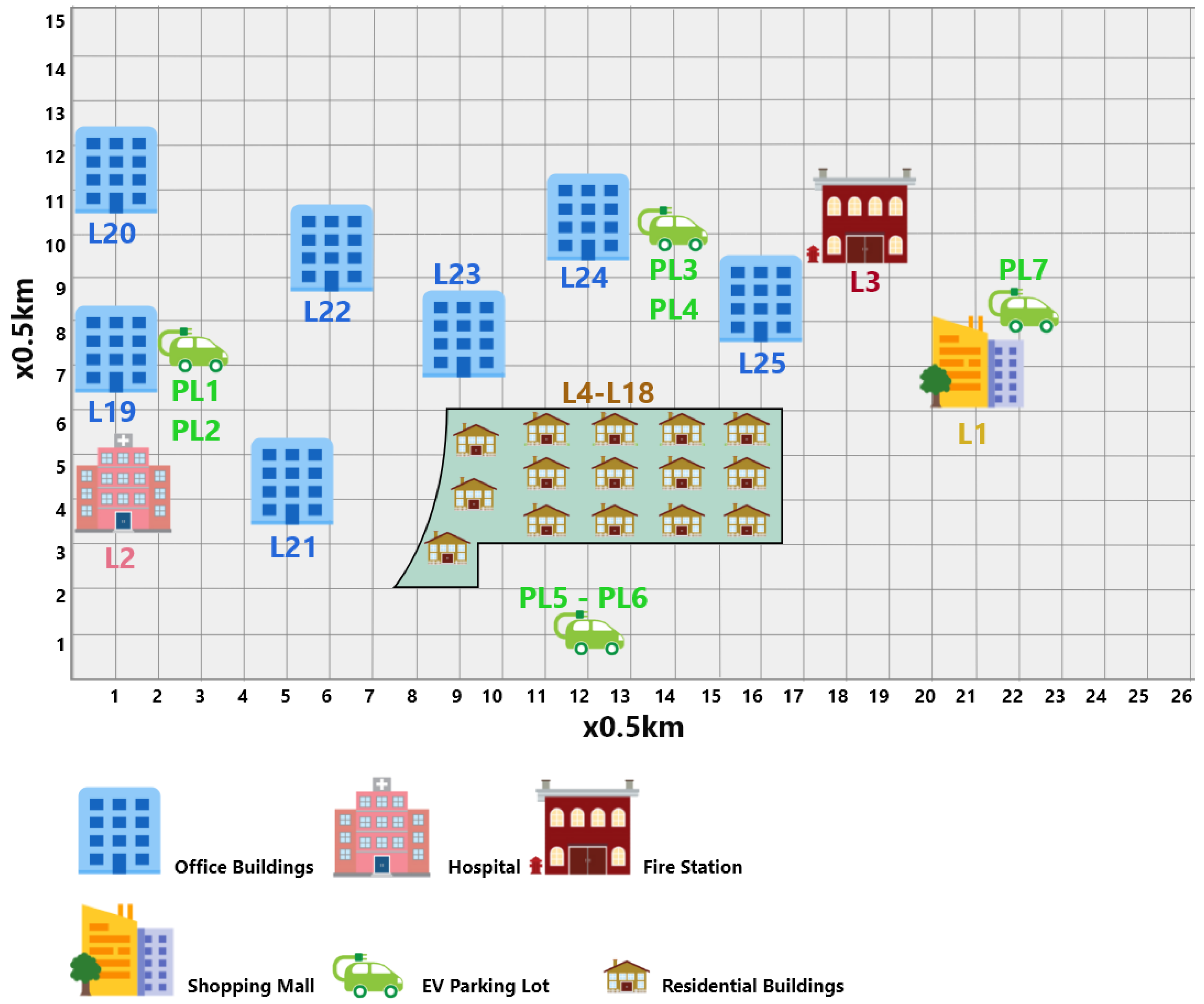
One of the goals of the slave subproblem is to verify the feasibility of the master problem. Moreover, through AC optimal power flow, the slave subproblem provides the optimal value for the operation variables. The slave subproblem objective function is represented by (26), where the operation costs and the slack variables ZA, ZQ, and ZF are minimized. Slack variables ZA and ZQ (for active and reactive power balance) and ZF (for thermal lines capacity) can take any positive value to make the optimization problem feasible. The value of these variables represents how much some constraints are being violated. The slave sub-problem cannot change the binary variables, but is free to explore the continuous variables in order to satisfy the several constraints, while minimizing the objective function and the value of the slack variables.
S O C = i Ω B j Ω B C o n g S ( i , j ) 2 + C o n g S ( i , j ) · C o s t C o n g + i Ω B S b P S u p p l i e r ( i ) · p r i c e M k + i Ω L b P N S s ( i ) · C o s t P N S + i Ω D G n d P P G C s ( i ) · P P G C C o s t + i Ω B j Ω B S L o s s ( i , j ) · C o s t L o s s + i Ω B Z A ( i ) + Z Q ( i ) · C o s t I n f + i Ω B Ω B i Z F ( i , j ) · C o s t I n f
The slave subproblem (26) is subjected to Constraints (27)–(52).
Network constraints
Voltage magnitude
The voltage magnitude of each bus is constrained by a maximum and minimum deviation (27).
V ( i ) m i n V ( i ) V ( i ) m a x i Ω B
Voltage angle
The maximum and minimum angle deviation is constrained by (28).
θ ( i ) m i n θ ( i ) θ ( i ) m a x i Ω B
Active power balance
Constraint (29) guarantees the active power balance in each distribution network bus.
i Ω D G n d P D G ( i ) P P G C s ( i ) + i Ω B S b P S u p p l i e r ( i ) i Ω L b P L o a d ( i ) P N S s ( i ) i Ω V b E V P ( i ) + i Ω B S b S T d c h S ( i ) S T c h S ( i ) i Ω B P I n j ( i ) + Z A ( i , j ) = 0
Reactive power balance
Constraint (30) guarantees the reactive power balance in each distribution network bus.
i Ω B S b Q S u p p l i e r ( i ) + i Ω C B b Q C b a n k s ( i ) i Ω L b Q L o a d ( i ) i Ω B Q I n j ( i ) + Z Q ( i , j ) = 0
Injected active power
This Equation (31) represents the injected active power in each bus of the network.
P I n j ( i ) = V ( i ) j Ω B V ( j ) G ( i , j ) · cos θ ( i , j ) + B ( i , j ) · sin θ ( i , j ) i Ω B , ( i , j ) Ω l
Injected reactive power
The injected reactive power in each bus is represented by the equation (32).
Q I n j ( i ) = V ( i ) j Ω B V ( j ) G ( i , j ) · sin θ ( i , j ) B ( i , j ) · cos θ ( i , j ) i Ω B , ( i , j ) Ω l
Active power flow
The active power flow for each network line is given by the equation (33).
P ( i , j ) = ( V ( i ) 2 V ( i ) · V ( j ) · cos θ ( i , j ) ) · G ( i , j ) ( V ( i ) · V ( j ) · sen θ ( i , j ) ) · B ( i , j ) i Ω B , j Ω B , ( i , j ) Ω l
Reactive power flow
Equation (34) gives the reactive power flow for each line.
Q ( i , j ) = ( V ( i ) 2 V ( i ) · V ( j ) · cos θ ( i , j ) ) · B ( i , j ) ( V ( i ) · V ( j ) · sen θ ( i , j ) ) · G ( i , j ) i Ω B , j Ω B , ( i , j ) Ω l
Apparent power flow
The apparent power flow equation, as can be seen in Equation (35), is given by the square root of the active power flow and reactive power flow squares.
S ( i , j ) = P ( i , j ) 2 + Q ( i , j ) 2 ( i , j ) Ω l
Active power losses
The active power loss of each line is represented by Equation (36).
P L o s s ( i , j ) = P ( i , j ) 2 + Q ( i , j ) 2 V ( i ) 2 · r ( i , j ) i Ω B , ( i , j ) Ω l
Reactive power losses
To represent the reactive power loss, the following Equation (37) is used.
Q L o s s ( i , j ) = P ( i , j ) 2 + Q ( i , j ) 2 V ( i ) 2 · x ( i , j ) i Ω B , ( i , j ) Ω l
Apparent power loss
To obtain the apparent power loss in each line, the following equation is used (38).
S L o s s ( i , j ) = P L o s s ( i , j ) 2 + Q L o s s ( i , j ) 2 ( i , j ) Ω l
Maximum admissible line flow
The maximum power flow in each line is constrained by (39).
0 F l o w S ( i , j ) F l o w ( i , j ) m a x + Z F ( i , j ) ( i , j ) Ω l
Supplier constraints
Maximum and minimum limits for active power supplier
The active power is constrained by the maximum and minimum capacity that can be supplied (40).
P S M i n L i m i t ( b s ) P S u p p l i e r ( b s ) P S M a x L i m i t ( b s ) b s Ω B S
Maximum and minimum limits for the reactive power supplier
The reactive power is constrained by the maximum and minimum capacity that can be supplied (41).
Q S M i n L i m i t ( b s ) Q S u p p l i e r ( b s ) Q S M a x L i m i t ( b s ) b s Ω B S
Maximum and minimum limits for capacitor banks
The reactive power of a capacitor bank is considered a continuous variable in this model and is constrained by the maximum and minimum (zero) capacity that can be supplied (42).
0 Q C b a n k s ( c b ) Q C b a n k s ( c b ) max c b Ω C B
Curtailment constraints
Power generation curtailment
Power generation curtailment occurs when the generator generates an excess of power g. This variable cannot be higher than the generation of the g generator (43).
0 P P G C s ( g ) P D G ( g ) g Ω D G n d
Power not supplied
Constraint (44) guarantees that the power not supplied variable must be lower or equal to the load demand.
0 P N S s ( l o ) P L o a d ( l o ) l o Ω L b
Lines’ congestion
Lines’ power congestion
The power congestion in each line is constrained by the Equation (45). The same considerations are taken into account in (15) and in (45).
C o n g ( i , j ) F l o w S ( i , j ) C o n g M i n · F l o w ( i , j ) m a x ( i , j ) Ω l C o n g ( i , j ) 0
Energy storage system constraints
Discharge limit of the energy storage systems
The maximum discharge limit determined by the constraint of each ESS (46).
S T d c h S ( e ) S T d c h R ( e ) e Ω E b , S T d c h S 0
Charge level limit for the energy storage systems
The maximum charge level limit determined by the constraint of each ESS (47).
S T c h S ( e ) S T c h R ( e ) e Ω E b , S T c h S 0
Discharge limit considering energy storage systems’ state
The maximum discharge limit considering the capacity constraint of each energy storage system (48). Δ t is represented in units of hours.
S T d c h S ( e ) · 1 d e f ( e ) S T s t o S ( e ) · 1 Δ t e Ω E b , S T d c h S 0
Charge limit considering energy storage systems’ capacity
The maximum charge level limit is determined considering the capacity constraint of each energy storage system (49). The Δ t is represented in units of hours.
S T s t o S ( e ) + S T c h S ( e ) · c e f ( e ) · 1 Δ t S T c a p ( e ) e Ω E b , S T c h S 0
State of charge of the energy storage systems
The state of charge of each ESS is given by (50). Δ t is represented in units of hours.
S T s t o S ( e ) Δ t · S T c h S ( e ) · c e f ( e ) + Δ t · S T d c h S ( e ) · 1 d e f ( e ) = S T s t o S ( e ) t 1 e Ω E b , S T c h S 0 , S T d c h S 0
Maximum energy storage systems’ capacity limit
The maximum capacity limit for each ESS is represented by (51).
S T s t o S e S T c a p ( e ) e Ω E b
Minimum energy storage systems’ capacity limit
The minimum capacity limit for each ESS is represented by (52).
S T s t o S ( e ) S T s t o S ( e ) min e Ω E b

3. Case Study

To show how the proposed methodology is applied, a medium voltage (MV) distribution network of an SC (mock-up) located at BISITE laboratory has been developed for this study (the schematic of the SC is presented in Figure 5, and the coordinates of each building can be seen in Table 3). In this case study, a high DER penetration is considered to represent a realistic scenario in the near future. The single-line diagram of the 13-bus 30-kV distribution network is presented in Figure 6.
This DN has one 30 MVA substation, 25 load points, and 3 × 35.88 km of underground cables. For the connections between the substation and the network (bus 1 to bus 2; bus 1 to bus 7), a cable of type LBHIOV 3 × 150 mm 2 (svrweb.cabelte.pt) has been used, while for the remaining connections, the cable type LBHIOV 3 × 70 mm 2 (svrweb.cabelte.pt) has been used. A total of 15 DG units (i.e., two wind farms and 13 PV parks) and four capacitor banks of 1 Mvar are included in the network, as can be seen in Figure 6.
The DG penetration corresponds to 27% (10.925 MW) of the total installed power (24% corresponds to wind generation and 3% to PV). Each wind farm has six E48 800 kW ENERCON wind turbines (www.enercon.de). The characteristics of PV parking lots are presented in Table 4. The line congestion cost was 0.02 €/kW when power flow was above 50% of the thermal line rating capacity ( C o n g M i n ).
The considered smart city presents five types of loads, namely:
  • Residential buildings (1375 homes);
  • Office buildings (seven buildings);
  • Hospital;
  • Fire Station;
  • Shopping Mall.
This study considered one week of input data for every 15-min period with the aim of showing the effectiveness of the proposed methodology (i.e., 672 periods were considered in the simulation process). The chosen week was 19 March 2017–25 March 2017. The total renewable generated power for each period is presented in Figure 7.
Figure 8 and Figure 9 present the power demand and the roof generation, respectively, of the office buildings, residential buildings, a shopping mall, a hospital, and a fire station. It is important to note that the power demand presented in these two figures corresponds to the subtraction of the initial demand for PV power generation, i.e., all the power generated by the PVs is consumed by the building. The generated power is therefore not sent to the grid in the present study.
The market price for the chosen week was obtained from the Iberian electricity market operator (OMIE) (www.datosdelmercado.omie.es/pt-pt/datos-mercado) and can be seen in Figure 10.
Moreover, the SC has seven parking lot buildings for EV charging, four (two in bus 7 and two in bus 11) slow charging lots (7.2 kW for each connection point) and three (two in bus 2 and one in bus 5) fast charging lots (50 kW for each connection point). Each slow charging parking lot has 250 spaces for EVs, while each fast charging parking lot has 80 spaces. In this case study, we assumed that each parking lot had a 30% occupation rate (OPR). Thus, in the following Equation (2), the additional cost related to the fixed term of network price rate to be charged to the customer (ACNR) for a slow charging parking space is 0.0132 €/kWh, while for a fast charging parking space, it is 0.0919 €/kWh. Furthermore, the parking owner charges an additional 5% fee and 23% of value-added tax (VAT). Moreover, consider that 50% of the EV users can charge their EV at home (3.7 kW charge point) with a fixed cost of 0.2094 €/kWh. A total of 5000 EVs were considered in this study, and the initial battery level was randomly generated between 40% and 65% of the battery capacity. The considered EV models and their characteristics are listed in Table 5. The weights (w1 and w2) attributed to the distance and price preference are presented in Table 6 and Table 7, respectively. Two possible scenarios are considered: in one, the user’s priority is to charge his/her EV at a charging station located as close as possible to them (Table 6); in the second scenario, the users prefer to find charging stations where they can charge their EV at a low price (Table 7).
Furthermore, two energy storage systems managed by the DSO were considered in the present case study, each one with 1 MWh of capacity and 0.5 MW of charge/discharge rate. Moreover, in this case, the ESS are able to charge at any moment and discharge when the energy market price is greater than or equal to 45 €/MWh. Is assumed that the ESS had a minimum of 5% of power stored, i.e., the power stored in the ESS cannot be less than 5%. The input data used in the case study can be found by the readers in [84].
In this research work, thirty different case studies were performed. Table 8 summarizes the characteristics of those studies. They have been divided into two types of EV user preference scenarios, namely the price preference scenario and distance preference scenario. For each of those scenarios, we considered DG, EV, ESS, dynamic EV charging price, and fixed prices (with three different price levels) and combined them in the case study. The purpose of these case studies was to determine in which situations dynamic charging prices were advantageous for DSO and EV users.

4. Results and Discussion

The proposed methodology has been applied to the case study presented in Section 3 to show its applicability. The proposed research work has been developed on a computer with one Intel Xeon E5-2620 v2 processor and 16 GB of RAM running Windows 10 Pro using the MATLAB R2016a and TOMLAB 8.1 64 bits with CPLEX and SNOPT solvers. As can be seen in Table 9, in each period, the optimization model dealt with the master problem, which had 566 constraints and 744 variables, where 171 were integer variables, and with the slave problem, which had 199 constraints (116 non-linear constraints) and 286 variables.
The average execution time was compatible with operation/reconfiguration time-frame, presenting an average value of 1.2 s (considering all case studies). The analysis of computer system resource impact was also evaluated with a memory test for which the MATLAB memory profiler tool was used. This tool shows the peak memory for each function in the code. The highest computer resource value is 4656 kB, which is perfectly compatible with today’s computers.
This section looks at the results of the analysis from two perspectives: that of the operator (Section 4.1) and that of the EV user (Section 4.2).

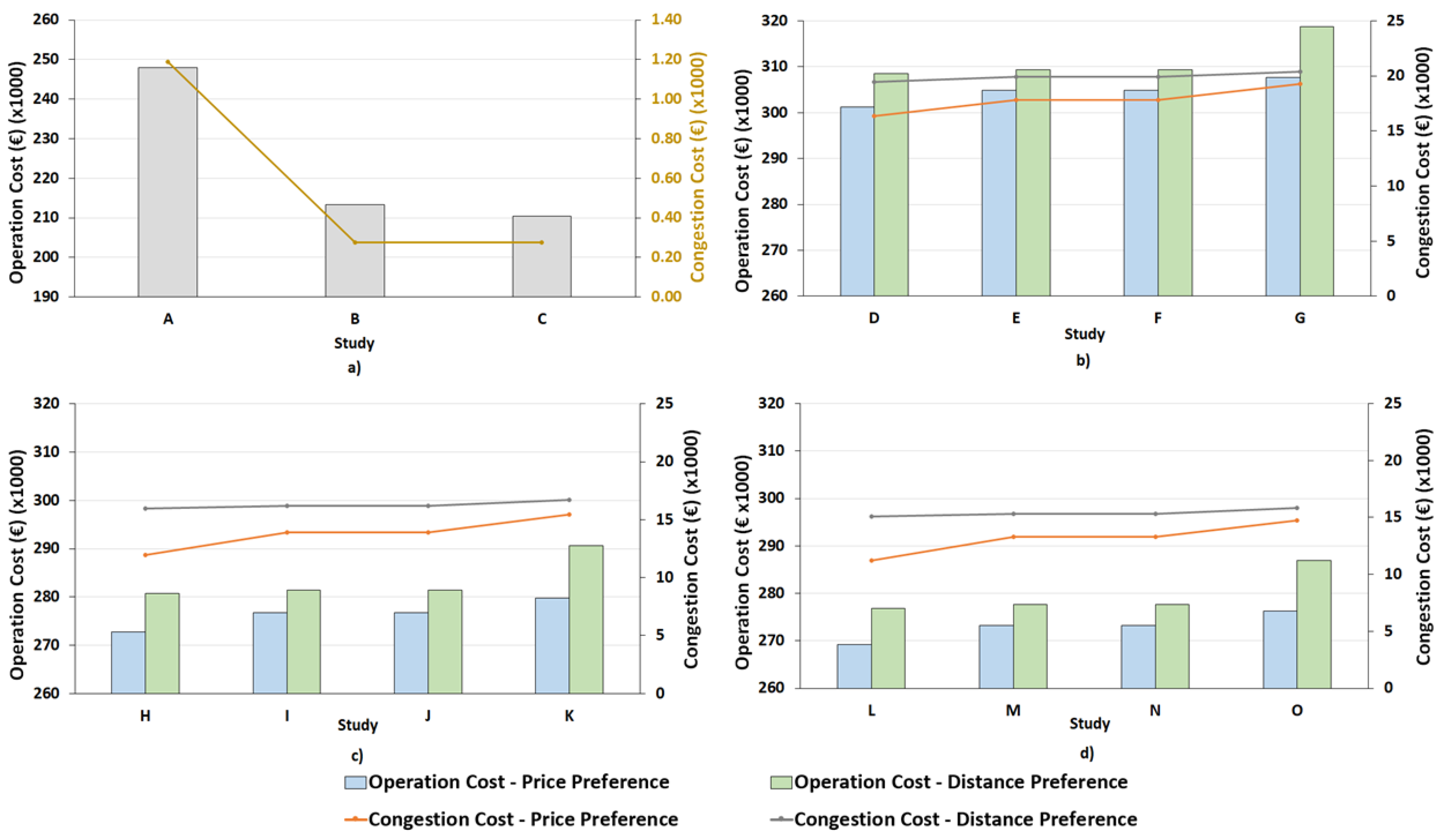
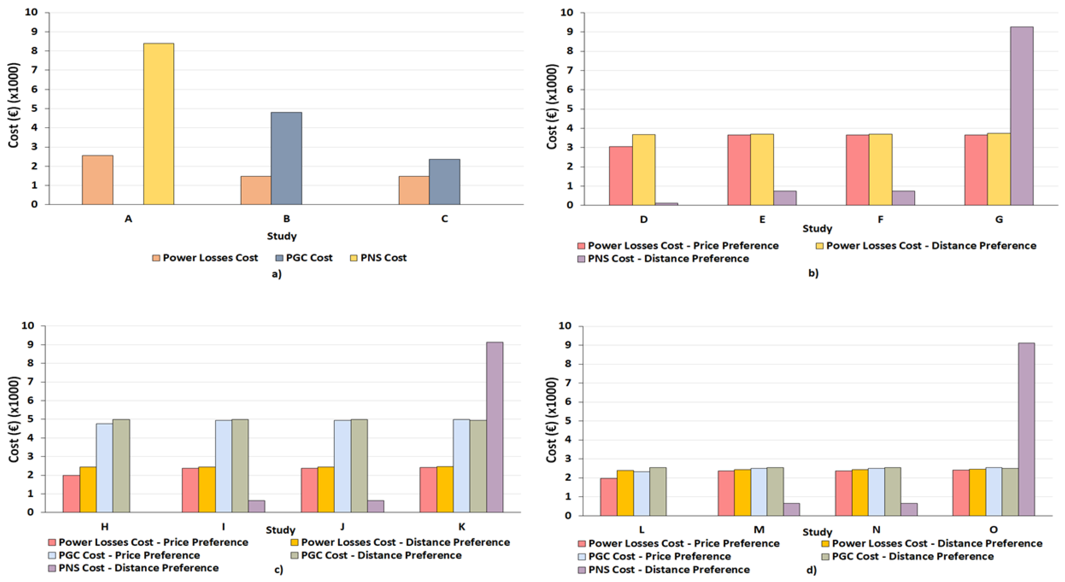
4.1. The Operator’s Perspective

In this subsection, the results are discussed from the perspective of the operator. Figure 11 presents the total operation and congestion cost (672 periods, one week) for all case studies. This figure makes evident the advantages in terms of cost when the DG and ESS systems are used in the network. (a) gives the total operation cost and the total congestion cost for the reference case, i.e., without EVs. Operation costs and congestion costs are reduced significantly when combined with distributed resources, namely with RES and ESS.
(b) (RES and ESS are not considered) verifies that with dynamic EV charging price, operation costs were reduced by 1.20%, 1.20%, and 2.10% when compared to the E, F, and G cases, respectively, for the user price preference scenario. In the user distance preference scenario, costs were reduced by 0.28%, 0.28%, and 3.20%. Moreover, congestion costs were reduced by 8.35%, 8.35%, and 15.20% thanks to dynamic EV charging prices in the user price preference scenario and by 2.29%, 2.29%, and 4.59% in the user distance preference scenario. From the analysis of (c) in Figure 11, compared to fixed prices (Cases I, J, and K), the dynamic EV charging prices presented a cost reduction in the user preference scenario by 1.43%, 1.43%, and 2.52% and in the user distance preference scenario by 0.24%, 0.24%, and 3.43%. Congestion costs were reduced by 13.87%, 13.87%, and 22.62% in the user price preference scenario and by 1.53%, 1.53%, and 4.60% in the user distance preference scenario. In (d), operation costs with fixed EV charging prices (Cases M, N, and O) were reduced by 1.47%, 1.47%, and 2.53% with dynamic EV charging prices. In the user distance preference scenario, cost was reduced by 0.29%, 0.29%, and 3.49%. Congestion costs were reduced by 5.25%, 15.25%, and 23.64% in the user price preference scenario and by 1.41%, 1.41%, and 4.48% in the user distance preference scenario. It is noted that there was no difference in operation costs between slow charging of 0.15 €/kWh or 0.20 €/kWh and fast charging of 0.25 €/kWh or 0.30 €/kWh. Thus, the operator was indifferent to the charging price for the EV user.
The use of dynamic prices for EV charging is beneficial in terms of reduced operation and congestion costs when compared to fixed price options. The reductions are more evident when the fixed prices are higher. Thanks to dynamic EV charging, different charging prices were offered to the users in the parking lots, and this helped alleviate certain power lines, contributing in this way to the operational cost reduction.
Total power loss, power generation curtailment, and power not supplied costs in each user preference scenario are presented in Figure 12a, i.e., with no electric vehicles. It has been verified that the costs associated with those three terms reduced once the distributed energy resources were included (RES and ESS). In fact, the power not supplied (PNS) cost was reduced to zero when the RES were considered alone or together with ESS. However, with RES and ESS, power generation curtailment (PGC) was present, but the costs were lower than with the PNS.
Through the analysis of (b) (RES and ESS were not considered) in Figure 12, it can be observed that the total power loss (PL) cost was equivalent to the three fixed-price cases with a cost of around 3662 € in the user price preference scenario. Through the use of the dynamic EV charging price method, the PL cost reduced by around 17%. Considering the user distance preference scenario, the dynamic EV charging prices presented a reduction of only 1.03% in Cases E and F and of 1.91% in Case G. The PNS occurred only in the user distance preference scenario. When the dynamic EV charging prices were included, the PNS cost was small compared to the fixed price (83.54% smaller than in Cases E and F and 98.67% smaller than in Case G). Considering the user price preference scenario in (c) of Figure 12, the observed PL cost reduction with dynamic energy pricing was of 16.75% in Cases I and J and 18.08% in Case K. Cost reductions were lower in the distance user preference scenario, reducing by 0.21% in Cases I and J and 1.52% in Case K. The PNS occurred only for the fixed price cases in the user distance preference scenario, being zero when the dynamic EV charging prices was used. The presence of RES will create the necessity of PGC in some periods. The dynamic EV charging prices can mitigate the costs associated with the PGC in the user price preference scenario, by 3.46% in Cases I and J and 4.32% in Case K. If the user distance preference scenario were considered, it would not be possible to benefit from dynamic EV charging prices. In (d), the presence of ESS was also considered, and its advantages in reducing PGC cost were evident. Through the use of dynamic EV charging prices, PL was reduced by 16.24% in Cases M and N and 18.03% in Case O in the user price preference scenario and by 2.19% in Cases M and N and 2.29% in Case O in the user distance preference scenario. With dynamic EV charging prices in the user price preference scenario, the PGC costs were reduced by 6.86% in Cases M and N and by 8.48% in Case O. In the user distance preference scenario, the cost of PGC did not reduce with dynamic EV charging prices. As can be seen, the use of dynamic EV charging prices is of great advantage in the PGC, leading to a zero value.
Once again, the conclusion drawn from the above analysis is that using dynamic energy pricing for EVs’ charging contributed greatly to a reduction in costs associated with power loss, power generation curtailment, and power not supplied. The reductions were more evident for PNS, where they reached 100% in Cases H and L.
Table 10 presents the maximum and the minimum voltage reached in each study. It also presents the buses where those values are verified. As can be seen in this table, the worst voltage values for the user price preference scenario and for the user distance preference scenario were verified in Case G at bus 6 and bus 5, respectively, mainly because these cases did not consider DG and ESS. When adopting dynamic pricing combined with the use of EVs (Cases D, H, and L in the user price preference scenario), it is possible to verify that this leads to better voltage levels (i.e., min. voltage), demonstrating the advantage of dynamic charging prices when EVs react to charging price.
Case L (which is a dynamic EV charging price case) and the case with 0.20 €/kWh for slow charge and 0.30 €/kWh for fast charge (fixed energy charging price) were chosen as an example to present the total energy charge consumption, the average charge power, and the preference percentages of the EV users for each bus that had parking lots. Figure 13 illustrates Case L, and Figure 14 presents the fixed price case.
The preference for a bus with an EV parking lot was counted from the moment the EV began to charge until the time it left the parking lot (one charging session).
In (a), it is possible to see that when the user price preference scenario was considered, the total energy consumed when charging an EV in bus 7 (slow charging parking lot) was 88,037 kWh, which in comparison to the other three buses was 69%, 88%, and 91% more, meaning that the energy price to charge at this bus was better than at the others. Thus, the average charging power followed the same trend as energy consumption. In the user distance preference scenario, energy consumption during charging was spread more evenly over the other parking lot buses. In this case, the highest consumption was the one in bus 2 (fast charging parking lot) with around 45,500 kWh. This bus consumed 19%, 35%, and 14% more energy than the remaining parking lot buses. Once again, the average charge power followed the energy charge consumption trend.
Figure 13b,c shows the preference percentages of the EV users for each bus with a parking lot, considering the user price and distance preferences scenarios, respectively. Figure 13b shows that the parking lot located at bus 7 was the one preferred by EV users, with 69.04% of charged EVs. The parking lot located in bus 11 was the second most chosen, while the fast charging parking lots were the ones least used, with a total of 4.85%. The slow charging parking lots were those that had the lowest energy charging price when compared to the fast charging parking lots. Then, since the user price preference scenario is being considered here, the choice of the less expensive parking lot was logical.
In Figure 13c, the user distance preference scenario is considered. In this scenario, the user preference was to find a parking lot that was as close as possible to the total route that the user would have to travel, i.e., the lowest summation distance between the current EV location and the parking lot and the distance between the parking lot and the next destination. In this user preference scenario, the fast charging parking lots obtained a higher preference when compared to the case where the user preference was defined by the price. This indicates that when the price was not the most important factor, fast charging parking lots could attract users who were located close to them. Nevertheless, we arrived at the conclusion that the location of those parking lots was not optimal, because even when considering the user distance preference scenario, the majority of the users chose the slow charging parking lots: the lease expensive ones.
It is also important to note in the user distance preference scenario that even the parking lots located at bus 11 presented higher user charging preference when compared to the parking lots located at bus 7; the energy consumption and the average charging power at the parking lots of bus 11 were not higher than those at bus 7. This means that the energy price in bus 11 presented higher variations, and it was worse in general when compared to the energy price in bus 7 (it is possible to observe this in Section 4.2, second box plot figure), which contributed to higher energy charge consumption in bus 7 and a considerable charging preference (37.35%) even though there was only a 30% probability in the user price preference scenario (see Table 6). Moreover, due to the higher charge preference at bus 11, it is possible to conclude that the location of the parking lots at this bus was better (advantageous because EV users were at a shorter distance from them) when compared to the parking lots at bus 7.
The total energy charge consumption, the average charge power, and the preference percentages of the EV users for the fixed energy prices (0.20 €/kWh for slow charge and 0.30 €/kWh for fast charge) are presented in Figure 14.
In Figure 14a, it can be observed that in the user price preference scenario, the bus with the highest total energy consumption for EV charging was bus 11 with 40,733 kWh, that is 9%, 28%, and 13% more than buses 7, 2, and 5, respectively. Thus, the average charging power followed the same trend of the energy consumed during charging. In comparison, (a) in Figure 13 shows that the energy consumed by the charging EVs was spread more evenly among all the parking lot buses, while in the dynamic EV charging price case, energy consumption due to charging was more concentrated in bus 7 than the others. This means that bus 7 with respect to dynamic EV charging price presented a better charging price. In the user distance preference scenario, the energy charge consumption followed the same trend as in the dynamic EV charging price case, indicating energy consumption of 50,815 kWh at bus 2; the consumption was higher by 42%, 38%, and 21% in relation to the remaining buses. Regarding the average charging power, the trend was the same as for energy consumption.
Analyzing Figure 14b, which presents the preference percentages of the EV users for each bus with parking lots, considering the user price preference scenario, it can be seen that the parking lot in 11 was preferred among users with 49.34% of EV users choosing this lot. The parking lots located at bus 7 were in second place, while the fast charging parking lots had a total of around 19% preference among users, quite higher when compared with (b) of Figure 13. This means that in the dynamic EV charging price case, the most attractive prices were on the buses that had slow charging parking lots, leading to a great number of users choosing them over the fast charging parking lots. The majority of the users preferred slow charging due to the lower charging price (0.20 €/kWh).
Once again, in the user distance preference scenario, the fast charging parking lots were a more popular choice among users than in the user price preference scenario ((c) of Figure 14)). This also indicates that those parking lots could attract users who find themselves closer to the fast charging parking lots, if the price is not the most important factor. However, we arrived at the conclusion that those parking lost cannot be located optimally because the slow charging parking lots were highly preferred among users due to more attractive EV charging prices (even in the user distance preference scenario).

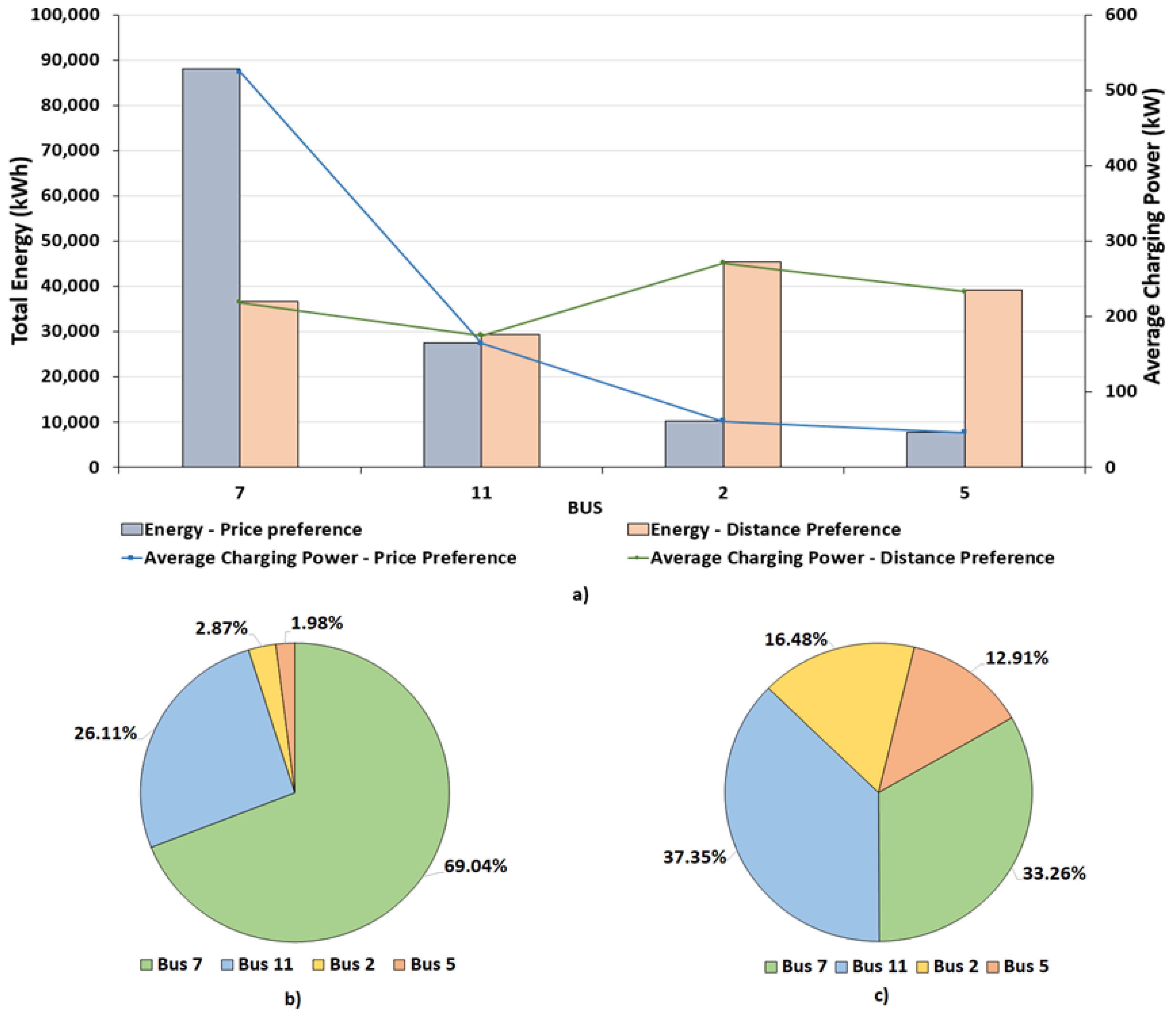
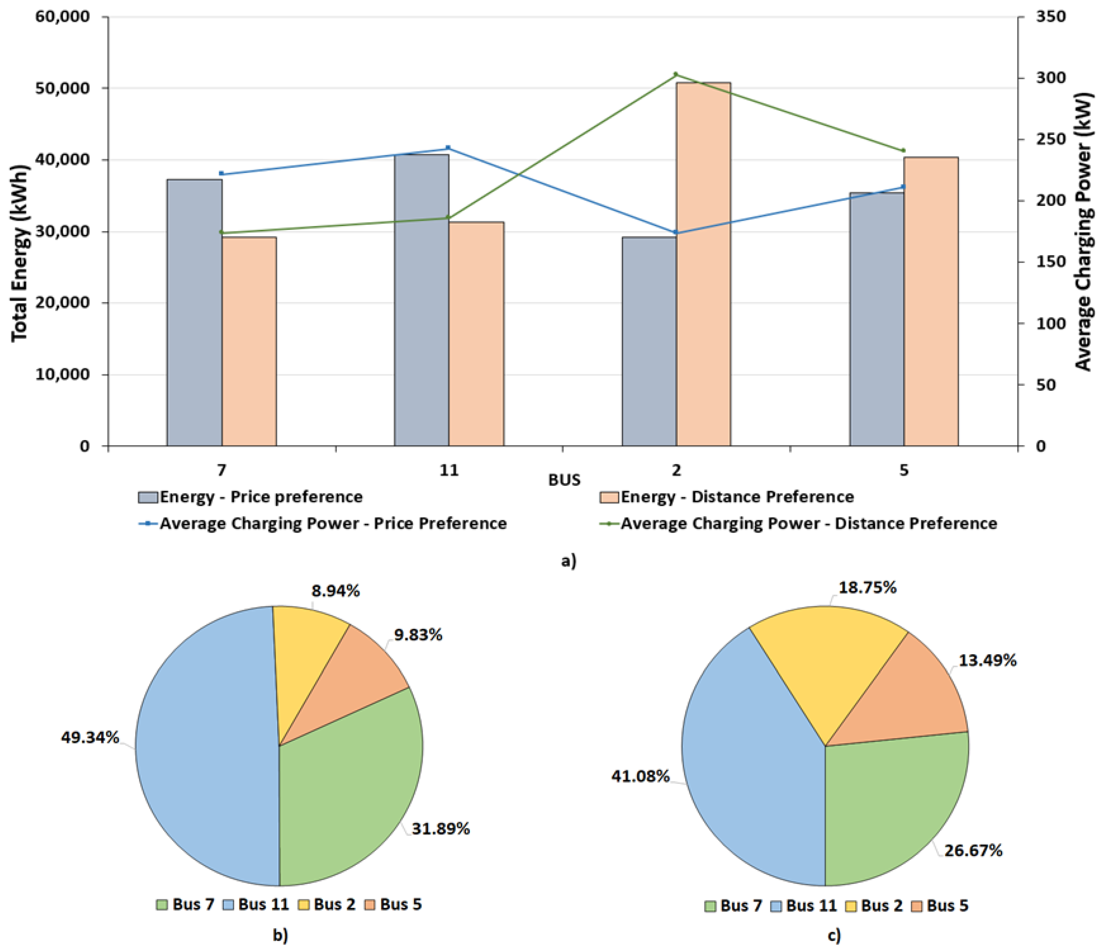
4.2. User Perspective

This subsection looks at the results of the case studies from the perspective of the EV users. Figure 15 and Figure 16 present the box plots for the dynamic EV charging price cases considering the user price and distance preference scenarios, respectively. By comparing these two figures, it is possible to see that the differences between the same cases in each figure were small. The verified variations were mainly in Quartile 3 (Q3) and were higher in the user price preference scenario, in which the users gave priority to price.
Let us take bus 11 in Case L as an example: it can be seen that the charge price variation in the user price preference scenario was between 0.0990 €/kWh and 0.2150 €/kWh, while in the user distance preference scenario, it was between 0.0990 €/kWh and 0.2000 €/kWh, corresponding to a 0.0150 €/kWh of difference. Fifty percent of the charge price values (interquartile range) were located between 0.1210 €/kWh and 0.1600 €/kWh for the user price preference scenario and between 0.1210 €/kWh and 0.1510 €/kWh for the user distance preference scenario (0.0090 €/kWh of difference). Twenty-five percent of the values varying between 0.0990 €/kWh and 0.1210 €/kWh for both user preference scenarios were located in the first quartile (Q1). Seventy five percent of the EV charging price values were represented by the third quartile (Q3) and varied between 0.0990 €/kWh and 0.1600 €/kWh in the user price preference scenario and between 0.0990 €/kWh and 0.1510 €/kWh in the user distance preference scenario. These two figures show that the highest variation in the charge prices among the dynamic EV charging price cases occurred specifically in slow charge buses in Case D. This is mainly due to the wind farms (one of them at bus 7 and the other one at bus 11, corresponding to 24% of the total installed power), which were not considered in Case D (it did not consider RES nor ESS).
Table 11 presents the results collected over a one-week period during which the case study was conducted; the average prices paid by EV users in the case of both dynamic EV charging prices and fixed charging prices. In these average prices values, the home charging price is included (0.2094 €/kWh). All dynamic EV charging price cases in the user price preference scenario show that the prices paid by EV users for EV charging were on average lower than what EV users normally would pay if the charging prices were fixed. However, this was not the case in the user distance preference scenario. To better understand the values presented in this table, let us analyze Table 12, Table 13 and Table 14, which stress the dynamic EV charging price cases with their homologous fixed price cases, presenting the gains in terms of the percentage of the EV users.
In Table 12, it is possible to see that the dynamic EV charging price Case D for the user price preference scenario presented gains of 4.03%, 16.63%, and 33.79% over all the homologous fixed price cases (E, F, and G), respectively. Even comparing a dynamic EV charging price case that did not consider distributed resources with the lowest fixed prices case (0.15 €/kWh for slow charge and 0.25 €/kWh for fast charge) verified the charge prices’ advantages. Regarding the user distance preference scenario, the dynamic EV charging price case did not present advantages in terms of charge price for the EV users when compared with fixed Cases E and F, which had 0.15 €/kWh for slow charge and 0.25 €/kWh for fast charge and 0.20 €/kWh for slow charge and 0.30 €/kWh for fast charge, respectively. Comparing with these two fixed prices cases, if the dynamic EV charging price were applied, the EV users would have had a loss of 15.66% and 1.88%, respectively, but obtained a gain of 18.30% when compared with the fixed charge price Case G.
Case H also presented charge price gains when compared with the homologous fixed charge prices, as can be seen in Table 13. In this case, the gains were 6.42%, 17.73%, and 35.45%, respectively, and when compared with Case D, it is possible to see a growth in those gains. For the user distance preference scenario, it can be seen that the dynamic EV charging prices were not also advantageous for the EV users when compared with the lowest considered fixed energy charge prices, but with a strong reduction when compared with the case that did not consider RES. Furthermore, a gain of 8% can be seen with Case H (a growth of 9.88%) over the charge fixed energy price considered for Case J (0.20 €/kWh for slow charge and 0.30 €/kWh for fast charge), as well as a growth of 7.92% over the 0.30 €/kWh (slow charge) and 0.40 €/kWh (fast charge) fixed charge prices.
With the RES and ESS presented in the distribution network, the results’ tendency was similar to Case H. Comparing the differences, it is possible to see through Table 14 that the gains of Case L were higher than the gains of Case H, namely due to the ESS consideration.

5. Conclusions

In this research work, the authors investigated if the dynamic EV charging prices have a positive impact on the smart distribution network operation and on the EV user behavior. To this end, the authors combined an EV behavior simulator with a proposed innovative smart DLMP-based distribution network operation/reconfiguration. The main contributions of the conducted study can be summarized as follows: (a) an EV user behavior simulator has been adopted to generate a realistic population, considering the network size and parking lots; (b) a distribution network operation/reconfiguration optimization model has been created in an SG context with high DER penetration concerning the behavior of the EV users and the dynamic EV charging price considering DLMPs using the Benders decomposition method; (c) the positive impact of the dynamic EV charging prices on the smart distribution network operation and on the electric vehicles users has been assessed.
The proposed methodology was tested in a case study, which has been conducted on a mock-up model of an SC located at the BISITE laboratory with a 13-bus distribution network. Furthermore, the distribution network operation/reconfiguration optimization model considering two user preference scenarios (price and distance preference) and using the dynamic EV charging prices were compared with the model using the EV fixed charging prices to demonstrate the advantage of the former.
It was verified that the use of dynamic pricing for EV charging is advantageous for the network operator in all of the considered cases due to reduced cost of operation and the user preference scenarios. These benefits are even more evident when considering high fixed charging prices (0.30 €/kWh for slow charging and 0.40 €/kWh for fast charging, −35.79% in the user price preference scenario, Case L). The lowest cost reduction was 0.24% in Case H of the distance preference scenario. Moreover, when the distance preference scenario and dynamic price were considered, it was verified that the PNS was zero, with exception of Case D, which presented an insignificant value (123.35 €).
For the EV users, the dynamic pricing also presented considerable cost advantages, namely when the price preference was considered. In this scenario, the lowest advantage (4.03% better) was verified in Case D compared with the lowest considered fixed charging prices (0.15 €/kWh for slow charge and 0.25 €/kWh for fast charge). Furthermore, for this scenario, the advantages can reach 35.75% (Case L), i.e., around 0.10 €/kWh of savings if the fixed charging prices are 0.30 €/kWh for slow charge and 0.40 €/kWh for fast charge. If the distance preference was considered, the dynamic EV charging price cases did not present savings in comparison with the lowest fixed charging price cases, namely when the fixed charging prices were 0.15 €/kWh for slow charge and 0.25 €/kWh for fast charge. Here, the user lost up to 15.66% for the dynamic EV charging price Case D. Nevertheless, the dynamic price still presented considerable savings when fixed prices were higher, reaching up to 26.30%.
The results suggest that the dynamic energy pricing for EVs’ charge can be used as an efficient approach in smart cities that allows important monetary savings for both the distribution system operator and EV users.
The main drawbacks of the proposed work are: (a) the EV users’ profiles were not adapted to the different weekdays; (b) the decision charge method was only based on the battery charge level; (c) vehicle-to-grid was not considered; (d) the ESS charge/discharge decision was limited and based on rules.
As future work, the authors suggest this research work include more EV user profiles, an additional charging decision method that depends on the energy price, an optimized ESS charge/discharge decision, an optimization model for EV users’ costs minimization, solar-powered charging infrastructures in the parking lots, and also the possibility of vehicle-to-grid.

Author Contributions

Conceptualization, B.C. and J.S.; Data curation, B.C.; Formal analysis, B.C. and J.S.; Investigation, B.C.; Methodology, B.C. and J.S.; Project administration, Z.V.; Resources, Z.V. and J.M.C.; Software, B.C.; Supervision, Z.V. and J.M.C.; Validation, B.C.; Visualization, B.C. and J.S.; Writing—original draft, B.C.; Writing—review and editing, B.C., J.S., Z.V. and J.M.C.

Funding

This research has received funding from FEDER funds through the Operational Programme for Competitiveness and Internationalization (COMPETE 2020), under Project POCI-01-0145-FEDER-028983; and by National Funds through the FCT—Portuguese Foundation for Science and Technology, under Projects PTDC/EEI-EEE/28983/2017 (CENERGETIC), UID/EEA/00760/2019, and SFRH/BD/110678/2015 PhD scholarship.

Acknowledgments

This work has received funding from FEDER Funds through the COMPETE program, from National Funds through FCT under the project UID/EEA/00760/2019 and from the project PTDC/EEI-EEE/28983/2017-CENERGETIC. Bruno Canizes is supported by FCT Funds through the SFRH/BD/110678/2015 PhD scholarship.

Conflicts of Interest

The authors declare no conflict of interest.

Abbreviations

The following abbreviations are used in this manuscript:
DERDistributed energy resources
DGDistributed generators
DLMPLocational marginal pricing
DNDistribution network
DNRDistribution network reconfiguration
DSODistribution system operator
ESSEnergy storage systems
EUEuropean Union
EVElectric vehicle
FChFast charge
LMPLocational marginal pricing
MINLPMixed-integer nonlinear programming
MOCMaster subproblem objective function
MVMedium voltage
OMIEIberian electricity market operator
PGCPower generation curtailment
PLPower losses
PNSPower not supplied
PVPhotovoltaic
RESRenewable energy sources
SCSmart city
SChSlow charge
SGSmart grid
VATValue-added tax
Indices
cLine options
iElectrical buses
jElectrical buses
l o Loads
b s External supplier
c b Capacitor bank
gDistributed generator unit
eEnergy storage systems
vElectric vehicles parking lot
mBender’s cuts iteration
Parameters
P P G C C o s t Power generation curtailment cost [€/MW]
p r i c e M K Market price [€/MWh]
C o s t P N S Power not supplied cost [€/MW]
C o s t L o s s Power losses cost [€/MW]
c e f Charge efficiency of energy storage systems
d e f Discharge efficiency of energy storage systems
C o s t C o n g Lines congestion cost [€/MW]
p r i c e M k Market price [€/MW]
C o s t P N S Power not supplied cost [€/MW]
r ( i , j ) Resistance for i,j line[ Ω ]
C o s t L o s s Power losses cost [€/MW]
P P G C C o s t Power generation curtailment [€/MW]
p D G ( g ) Power generation for g DG unit [MW]
E V P ( i ) Power charge for EV parking lot in the bus i [MW]
F l o w m a x ( i , j ) Maximum admissible line flow between bus i and bus j [MW]
n D G Number of DG units
E x t S u p M i n L i m i t ( b s ) Minimum limit of power supplied by substation/supplier bs [MW]
E x t S u p M a x L i m i t ( b s ) Maximum limit of power supplied by substation/supplier bs [MW]
p D G ( g ) Generated power of distributed generation g [MW]
p L o a d ( l o ) Active power demand for load lo [MW]
C o n g M i n Power congestion factor
S T d c h R ( e ) ESS discharge rate [MW]
S T c h R ( e ) ESS charge rate [MW]
S T d M ( e ) s t a t Decision for ESS e discharge {0,1}
S T c a p ( e ) ESS e capacity [MWh]
S T d M ( e ) s t a t Decision for ESS e discharge {0,1}
Δ t Duration of the period [hours]
S T s t o M ( e ) t 1 Energy stored in e ESS in previous period for master subproblem [MWh]
S T s t o S ( e ) t 1 Energy stored in e ESS in previous period for slave subproblem [MWh]
S T s t o ( e ) min Minimum capacity limit of the ESS e
p r i c e min M k Minimum market price value that will permit the ESS discharge
λ ( i , j ) m 1 Sensitivities associated to the radiality decision taken by the master problem in the previous iteration
μ ( i ) m 1 Sensitivities associated to the ESS charge decision taken by the master problem in the previous iteration
C o s t I n f Slave problem infeasibilities cost [€]
V ( i ) m i n Minimum voltage magnitude limit in the bus i [V]
V ( i ) m a x Maximum voltage magnitude limit in the bus i [V]
θ ( i ) m i n Minimum voltage angle limit in the bus i [rad]
θ ( i ) m a x Maximum voltage angle limit in the bus i [rad]
Q L o a d ( l o ) Reactive power demand for load lo [Mvar]
Q C b a n k s ( c b ) max Maximum limit of the capacitor bank cb [Mvar]
G ( i , j ) Real term of the element i,j in the bus admittance matrix
B ( i , j ) Imaginary term of the element i,j in the bus admittance matrix
x ( i , j ) Reactance for i,j line [ Ω ]
P s M i n L i m i t ( b s ) Minimum limit of active power supplied by substation/supplier bs [MW]
P s M a x L i m i t ( b s ) Maximum limit of active power supplied by substation/supplier bs [MW]
Q s M i n L i m i t ( b s ) Minimum limit of reactive power supplied by substation/supplier bs [Mvar]
Q s M a x L i m i t ( b s ) Maximum limit of reactive power supplied by substation/supplier bs [Mvar]
Variables
D g Fictitious load for each distributed generator g
E x t S u p ( b s ) Power supplied by substation bs [MW]
P N S M ( l o ) Power not supplied for load lo in the master subproblem [MW]
F l o w M ( i , j ) Power flow in the line i,j for the master subproblem [MW]
P P G C M ( g ) Power generation curtailment for master subproblem in the g DG unit [MW]
ω * Linear Benders’ cut variable
S T d c h M ( e ) Power discharge of ESS e for master subproblem [MW]
S T c h M ( e ) Power charge of ESS e for master subproblem[MW]
X ( i , j ) s t a t Binary decision variable {0,1} for the line usage between bus i and bus j
d i , j Fictitious flow associated with branch i,j
C o n g M i , j Power congestion for line i,j in the master subproblem [MW]
S T c M ( e ) s t a t Binary decision variable {0,1} for ESS e charge
S T d M ( e ) s t a t Binary decision variable {0,1} for ESS e discharge
S T s t o M ( e ) Energy stored in e ESS for master subproblem [MWh]
Z u p m 1 Sum of the infeasibilities of the slave problem
Z A Slack variable for active power balance
Z Q Slack variable for reactive power balance
Z F Slack variable for thermal lines capacity
C o n g S ( i , j ) Power congestion for line i,j in the salve subproblem [MW]
P S u p p l i e r ( b s ) Active power supplied by substation bs[MW]
Q S u p p l i e r ( b s ) Reactive power supplied by substation bs[Mvar]
P P G C s ( g ) Power generation curtailment for slave subproblem in the g DG unit [MW]
P N S s ( l o ) Power not supplied for slave subproblem in the load lo [MW]
S L o s s ( i , j ) Apparent power loss in the line i,j [MVA]
V ( i ) Voltage magnitude in the bus i [V]
θ ( i ) Voltage angle in the bus i [rad]
P I n j ( i ) Active injected power in the bus i [MW]
Q I n j ( i ) Reactive injected power in the bus i [Mvar]
Q C b a n k s ( c b ) Reactive power from capacitor bank cb [Mvar]
P ( i , j ) Active power flow in the i,j line [MW]
Q ( i , j ) Reactive power flow in the i,j line [Mvar]
S ( i , j ) Apparent power flow in the i,j line [MVA]
P L o s s ( i , j ) Active power loss in the i,j line [MW]
Q L o s s ( i , j ) Reactive power loss in the i,j line [Mvar]
F l o w S ( i , j ) Power flow in the i,j line for slave subproblem [MW]
S T d c h S ( e ) Power discharge of ESS e for slave subproblem [MW]
S T c h S ( e ) Power charge of ESS e for slave subproblem[MW]
S T s t o S ( e ) Energy stored in e ESS for slave subproblem [MWh]
D E P Dynamic EV charging price for each period [€/kWh]
T a r i f f M V Energy tariff price for each period [€/kWh]
P L G Additional profit margin of the parking owner
A C N R Additional cost related to the fixed term of network price rate to be charged to the customer [€/kWh]
Sets
Ω B Set of buses
Ω b B S Set of substation buses
Ω b C B Set of capacitor banks buses
Ω b L Set of load buses
Ω b E Set of ESS buses
Ω b V Set of EV parking lot buses
Ω B S Set of substations
Ω C B Set of capacitor banks
Ω l Set of lines
Ω n d D G Set of non-dispatchable DG buses

References

  1. Mokryani, G.; Hu, Y.F.; Papadopoulos, P.; Niknam, T.; Aghaei, J. Deterministic approach for active distribution networks planning with high penetration of wind and solar power. Renew. Energy 2017. [Google Scholar] [CrossRef]
  2. The European Union Leading in Renewables. Available online: https://ec.europa.eu/energy/sites/ener/files/documents/cop21-brochure-web.pdf (accessed on 8 February 2019).
  3. Paaso, A.; Kushner, D.; Bahramirad, S.; Khodaei, A. Grid Modernization Is Paving the Way for Building Smarter Cities [Technology Leaders]. IEEE Electr. Mag. 2018, 6, 6–108. [Google Scholar] [CrossRef]
  4. Curiale, M. From smart grids to smart city. In Proceedings of the IEEE 2014 Saudi Arabia Smart Grid Conference (SASG), Jeddah, Saudi Arabia, 14–17 December 2014; pp. 1–9. [Google Scholar] [CrossRef]
  5. Tuballa, M.L.; Abundo, M.L. A review of the development of Smart Grid technologies. Renew. Sustain. Energy Rev. 2016, 59, 710–725. [Google Scholar] [CrossRef]
  6. Kazmi, S.A.A.; Shahzad, M.K.; Khan, A.Z.; Shin, D.R. Smart Distribution Networks: A Review of Modern Distribution Concepts from a Planning Perspective. Energies 2017, 10, 501. [Google Scholar] [CrossRef]
  7. Blesl, M.; Das, A.; Fahl, U.; Remme, U. Role of energy efficiency standards in reducing CO2 emissions in Germany: An assessment with TIMES. Energy Policy 2007. [Google Scholar] [CrossRef]
  8. Erickson, L.E.; Robinson, J.; Brase, G.; Cutsor, J. Solar Powered Charging Infrastructure for Electric Vehicles: A Sustainable Development; CRC Press: Boca Raton, FL, USA, 2016. [Google Scholar]
  9. Alam, M.M.; Mekhilef, S.; Seyedmahmoudian, M.; Horan, B. Dynamic Charging of Electric Vehicle with Negligible Power Transfer Fluctuation. Energies 2017, 10, 701. [Google Scholar] [CrossRef]
  10. Foley, A.M.; Winning, I.; O Gallachoir, B.; Ieee, M. State-of-the-art in electric vehicle charging infrastructure. In Proceedings of the IEEE Vehicle Power and Propulsion Conference, Lille, France, 1–3 September 2010. [Google Scholar] [CrossRef]
  11. Heydt, G.T. The Impact of Electric Vehicle Deployment on Load Management Strategies. IEEE Power Eng. Rev. 1983. [Google Scholar] [CrossRef]
  12. Rahman, S.; Shrestha, G.B. An investigation into the impact of electric vehicle load on the electric utility distribution system. IEEE Trans. Power Deliv. 1993. [Google Scholar] [CrossRef]
  13. Salihi, J.T. Energy Requirements for Electric Cars and Their Impact on Electric Power Generation and Distribution Systems. IEEE Trans. Ind. Appl. 1973, IA-9, 516–532. [Google Scholar] [CrossRef]
  14. Geske, M.; Komarnicki, P.; Stötzer, M.; Styczynski, Z.A. Modeling and simulation of electric car penetration in the distribution power system—Case study. In Proceedings of the 2010 Modern Electric Power Systems, Wroclaw, Poland, 20–22 September 2010; pp. 1–6. [Google Scholar]
  15. Juanuwattanakul, P.; Masoum, M.A. Identification of the weakest buses in unbalanced multiphase smart grids with plug-in electric vehicle charging stations. In Proceedings of the 2011 IEEE PES Innovative Smart Grid Technologies, ISGT Asia 2011 Conference: Smarter Grid for Sustainable and Affordable Energy Future, Perth, WA, Australia, 13–16 November 2011. [Google Scholar] [CrossRef]
  16. Zhang, C.; Chen, C.; Sun, J.; Zheng, P.; Lin, X.; Bo, Z. Impacts of Electric Vehicles on the Transient Voltage Stability of Distribution Network and the Study of Improvement Measures. In Proceedings of the IEEE PES Asia-Pacific Power and Energy Engineering Conference, Hong Kong, China, 7–10 December 2014. [Google Scholar] [CrossRef]
  17. Dharmakeerthi, C.H.; Mithulananthan, N.; Saha, T.K. Impact of electric vehicle fast charging on power system voltage stability. Int. J. Electr. Power Energy Syst. 2014. [Google Scholar] [CrossRef]
  18. Ul-Haq, A.; Cecati, C.; Strunz, K.; Abbasi, E. Impact of Electric Vehicle Charging on Voltage Unbalance in an Urban Distribution Network. Intell. Ind. Syst. 2015, 1, 51–60. [Google Scholar] [CrossRef]
  19. De Hoog, J.; Muenzel, V.; Jayasuriya, D.C.; Alpcan, T.; Brazil, M.; Thomas, D.A.; Mareels, I.; Dahlenburg, G.; Jegatheesan, R. The importance of spatial distribution when analysing the impact of electric vehicles on voltage stability in distribution networks. Energy Syst. 2014. [Google Scholar] [CrossRef]
  20. Zhang, Y.; Song, X.; Gao, F.; Li, J. Research of voltage stability analysis method in distribution power system with plug-in electric vehicle. In Proceedings of the 2016 IEEE PES Asia-Pacific Power and Energy Engineering Conference (APPEEC), Xi’an, China, 25–28 October 2016; pp. 1501–1507. [Google Scholar] [CrossRef]
  21. Staats, P.T.; Grady, W.M.; Arapostathis, A.; Thallam, R.S. A statistical analysis of the effect of electric vehicle battery charging on distribution system harmonic voltages. IEEE Trans. Power Deliv. 1998. [Google Scholar] [CrossRef]
  22. Gómez, J.C.; Morcos, M.M. Impact of EV battery chargers on the power quality of distribution systems. IEEE Trans. Power Deliv. 2003. [Google Scholar] [CrossRef]
  23. Basu, M.; Gaughan, K.; Coyle, E. Harmonic distortion caused by EV battery chargers in the distribution systems network and its remedy. In Proceedings of the 39th International Universities Power Engineering Conferences, Bristol, UK, 6–8 September 2004. [Google Scholar]
  24. Jiang, C.; Torquato, R.; Salles, D.; Xu, W. Method to assess the power-quality impact of plug-in electric vehicles. IEEE Trans. Power Deliv. 2014. [Google Scholar] [CrossRef]
  25. McCarthy, D.; Wolfs, P. The HV system impacts of large scale electric vehicle deployments in a metropolitan area. In Proceedings of the 2010 20th Australasian Universities Power Engineering Conference, Christchurch, New Zealand, 5–8 December 2010. [Google Scholar]
  26. Putrus, G.; Suwanapingkarl, P.; Johnston, D.; Bentley, E.; Narayana, M. Impact of electric vehicles on power distribution networks. In Proceedings of the 2009 IEEE Vehicle Power and Propulsion Conference, Dearborn, MI, USA, 7–10 September 2009. [Google Scholar] [CrossRef]
  27. Fan, Y.; Guo, C.; Hou, P.; Tang, Z. Impact of Electric Vehicle Charging on Power Load Based on TOU Price. Energy Power Eng. 2013, 05, 1347–1351. [Google Scholar] [CrossRef]
  28. Di Silvestre, M.L.; Riva Sanseverino, E.; Zizzo, G.; Graditi, G. An optimization approach for efficient management of EV parking lots with batteries recharging facilities. J. Ambient Intell. Hum. Comput. 2013. [Google Scholar] [CrossRef]
  29. Sehar, F.; Pipattanasomporn, M.; Rahman, S. Demand management to mitigate impacts of plug-in electric vehicle fast charge in buildings with renewables. Energy 2017. [Google Scholar] [CrossRef]
  30. Hüls, J.; Remke, A. Coordinated charging strategies for plug-in electric vehicles to ensure a robust charging process. In Proceedings of the ACM 10th EAI International Conference on Performance Evaluation Methodologies and Tools, Taormina, Italy, 25–28 October 2017. [Google Scholar] [CrossRef]
  31. Biegel, B.; Andersen, P.; Stoustrup, J.; Bendtsen, J. Congestion Management in a Smart Grid via Shadow Prices. IFAC Proc. Volumes 2012. [Google Scholar] [CrossRef]
  32. Bohn, R.E.; Caramanis, M.C.; Schweppe, F.C. Optimal Pricing in Electrical Networks over Space and Time. RAND J. Econ. 1984. [Google Scholar] [CrossRef]
  33. Sotkiewicz, P.M.; Vignolo, J.M. Nodal pricing for distribution networks: Efficient pricing for efficiency enhancing DG. IEEE Trans. Power Syst. 2006. [Google Scholar] [CrossRef]
  34. Singh, R.K.; Goswami, S.K. Optimum allocation of distributed generations based on nodal pricing for profit, loss reduction, and voltage improvement including voltage rise issue. Int. J. Electr. Power Energy Syst. 2010. [Google Scholar] [CrossRef]
  35. Meng, F.; Chowdhury, B.H. Distribution LMP-based economic operation for future Smart Grid. In Proceedings of the 2011 IEEE Power and Energy Conference at Illinois, PECI 2011, Champaign, IL, USA, 25–26 February 2011. [Google Scholar] [CrossRef]
  36. Heydt, G.T.; Chowdhury, B.H.; Crow, M.L.; Haughton, D.; Kiefer, B.D.; Meng, F.; Sathyanarayana, B.R. Pricing and control in the next generation power distribution system. IEEE Trans. Smart Grid 2012. [Google Scholar] [CrossRef]
  37. Shaloudegi, K.; Madinehi, N.; Hosseinian, S.H.; Abyaneh, H.A. A novel policy for locational marginal price calculation in distribution systems based on loss reduction allocation using game theory. IEEE Trans. Power Syst. 2012. [Google Scholar] [CrossRef]
  38. O’Connell, N.; Wu, Q.; Østergaard, J.; Nielsen, A.H.; Cha, S.T.; Ding, Y. Day-ahead tariffs for the alleviation of distribution grid congestion from electric vehicles. Electric Power Syst. Res. 2012. [Google Scholar] [CrossRef]
  39. Li, R.; Wu, Q.; Oren, S.S. Distribution Locational Marginal Pricing for Optimal Electric Vehicle Charging Management. IEEE Trans. Power Syst. 2014, 29, 203–211. [Google Scholar] [CrossRef] [Green Version]
  40. Liu, W.; Wu, Q.; Wen, F.; Ostergaard, J. Day-ahead congestion management in distribution systems through household demand response and distribution congestion prices. IEEE Trans. Smart Grid 2014. [Google Scholar] [CrossRef]
  41. Huang, S.; Wu, Q.; Oren, S.S.; Li, R.; Liu, Z. Distribution Locational Marginal Pricing Through Quadratic Programming for Congestion Management in Distribution Networks. IEEE Trans. Power Syst. 2015. [Google Scholar] [CrossRef]
  42. Clement-Nyns, K.; Haesen, E.; Driesen, J. The impact of Charging plug-in hybrid electric vehicles on a residential distribution grid. IEEE Trans. Power Syst. 2010. [Google Scholar] [CrossRef]
  43. Leemput, N.; Geth, F.; Van Roy, J.; Delnooz, A.; Buscher, J.; Driesen, J. Impact of electric vehicle on-board single-phase charging strategies on a flemish residential grid. IEEE Trans. Smart Grid 2014. [Google Scholar] [CrossRef]
  44. Rezaee, S.; Farjah, E.; Khorramdel, B. Probabilistic analysis of plug-in electric vehicles impact on electrical grid through homes and parking lots. IEEE Trans. Sustain. Energy 2013. [Google Scholar] [CrossRef]
  45. Bin Humayd, A.S.; Bhattacharya, K. Assessment of distribution system margins to accommodate the penetration of plug-in electric vehicles. In Proceedings of the 2015 IEEE Transportation Electrification Conference and Expo, ITEC 2015, Dearborn, MI, USA, 14–17 June 2015. [Google Scholar] [CrossRef]
  46. Möller, F.; Meyer, J.; Schegner, P. Load model of electric vehicles chargers for load flow and unbalance studies. In Proceedings of the 9th International: 2014 Electric Power Quality and Supply Reliability Conference, PQ 2014—Proceedings, Rakvere, Estonia, 11–13 June 2014. [Google Scholar] [CrossRef]
  47. Min, Z.; Qiuyu, C.; Jiajia, X.; Weiwei, Y.; Shu, N. Study on influence of large-scale electric vehicle charging and discharging load on distribution system. In Proceedings of the IEEE 2016 China International Conference on Electricity Distribution (CICED), Xi’an, China, 10–13 August 2016; pp. 1–4. [Google Scholar] [CrossRef]
  48. Sarker, M.R.; Ortega-Vazquez, M.A.; Kirschen, D.S. Optimal Coordination and Scheduling of Demand Response via Monetary Incentives. IEEE Trans. Smart Grid 2015. [Google Scholar] [CrossRef]
  49. Mou, Y.; Xing, H.; Lin, Z.; Fu, M. Decentralized optimal demand-side management for PHEV charging in a smart grid. IEEE Trans. Smart Grid 2015. [Google Scholar] [CrossRef]
  50. Zou, S.; Ma, Z.; Liu, X.; Hiskens, I. An Efficient Game for Coordinating Electric Vehicle Charging. IEEE Trans. Autom. Control 2017. [Google Scholar] [CrossRef]
  51. Veldman, E.; Verzijlbergh, R.A. Distribution grid impacts of smart electric vehicle charging from different perspectives. IEEE Trans. Smart Grid 2015. [Google Scholar] [CrossRef]
  52. Li, C.; Schaltz, E.; Vasquez, J.C.; Guerrero, J.M. Distributed coordination of electric vehicle charging in a community microgrid considering real-time price. In Proceedings of the 2016 18th European Conference on Power Electronics and Applications, EPE 2016 ECCE Europe, Karlsruhe, Germany, 5–9 September 2016. [Google Scholar] [CrossRef]
  53. Akbari, H.; Fernando, X. Futuristic model of Electric Vehicle charging queues. In Proceedings of the IEEE 2016 3rd International Conference on Signal Processing and Integrated Networks (SPIN), Noida, India, 11–12 February 2016; pp. 789–794. [Google Scholar] [CrossRef]
  54. Wang, R.; Wang, P.; Xiao, G. Two-Stage Mechanism for Massive Electric Vehicle Charging Involving Renewable Energy. IEEE Trans. Veh. Technol. 2016. [Google Scholar] [CrossRef]
  55. Nguyen, H.N.T.; Zhang, C.; Zhang, J. Dynamic Demand Control of Electric Vehicles to Support Power Grid With High Penetration Level of Renewable Energy. IEEE Trans. Transp. Electr. 2016, 2, 66–75. [Google Scholar] [CrossRef]
  56. Jin, C.; Sheng, X.; Ghosh, P. Optimized Electric Vehicle Charging With Intermittent Renewable Energy Sources. IEEE J. Sel. Top. Signal Process. 2014, 8, 1063–1072. [Google Scholar] [CrossRef]
  57. Schuelke, A.; Erickson, K. The potential for compensating wind fluctuations with residential load shifting of electric vehicles. In Proceedings of the 2011 IEEE International Conference on Smart Grid Communications, SmartGridComm 2011, Brussels, Belgium, 17–20 October 2011. [Google Scholar] [CrossRef]
  58. Sourkounis, C.; Einwachter, F. Smart charge management of electric vehicles in decentralized power supply systems. In Proceedings of the IEEE 11th International Conference on Electrical Power Quality and Utilisation, Lisbon, Portugal, 17–19 October 2011; pp. 1–6. [Google Scholar] [CrossRef]
  59. Xiong, Y.; Chu, C.C.; Gadh, R.; Wang, B. Distributed optimal vehicle grid integration strategy with user behavior prediction. In Proceedings of the 2017 IEEE Power & Energy Society General Meeting, Chicago, IL, USA, 16–20 July 2017; pp. 1–5. [Google Scholar] [CrossRef]
  60. Gan, L.; Topcu, U.; Low, S.H. Optimal decentralized protocol for electric vehicle charging. IEEE Trans. Power Syst. 2013. [Google Scholar] [CrossRef]
  61. Wang, B.; Wang, Y.; Qiu, C.; Chu, C.C.; Gadh, R. Event-based electric vehicle scheduling considering random user behaviors. In Proceedings of the 2015 IEEE International Conference on Smart Grid Communications, SmartGridComm 2015, Miami, FL, USA, 2–5 November 2016. [Google Scholar] [CrossRef]
  62. Cao, Y.; Tang, S.; Li, C.; Zhang, P.; Tan, Y.; Zhang, Z.; Li, J. An optimized EV charging model considering TOU price and SOC curve. IEEE Trans. Smart Grid 2012. [Google Scholar] [CrossRef]
  63. Franke, T.; Krems, J.F. Interacting with limited mobility resources: Psychological range levels in electric vehicle use. Transp. Res. Part A Policy Pract. 2013, 48, 109–122. [Google Scholar] [CrossRef]
  64. Franke, T.; Bühler, F.; Cocron, P.; Neumann, I.; Krems, J.F. Enhancing Sustainability of Electric Vehicles: A Field Study Approach to Understanding User Acceptance and Behavior. Available online: https://www.tu-chemnitz.de/hsw/psychologie/professuren/allpsy1/pdf/Franke_et_al._2012_SustainEV.pdf (accessed on 8 February 2019).
  65. Franke, T.; Neumann, I.; Bühler, F.; Cocron, P.; Krems, J.F. Experiencing Range in an Electric Vehicle: Understanding Psychological Barriers. Appl. Psychol. 2012, 61, 368–391. [Google Scholar] [CrossRef]
  66. Franke, T.; Krems, J.F. Understanding charging behavior of electric vehicle users. Transp. Res. Part F Traffic Psychol. Behav. 2013, 21, 75–89. [Google Scholar] [CrossRef]
  67. Lu, X.; Chen, B.; Chen, C.; Wang, J. Coupled Cyber and Physical Systems: Embracing Smart Cities with Multistream Data Flow. IEEE Electr. Mag. 2018, 6, 73–83. [Google Scholar] [CrossRef]
  68. Hung, D.Q.; Mithulananthan, N. Loss reduction and loadability enhancement with DG: A dual-index analytical approach. Appl. Energy 2014, 115, 233–241. [Google Scholar] [CrossRef]
  69. Santos, S.F.; Fitiwi, D.Z.; Cruz, M.R.; Cabrita, C.M.; Catalão, J.P. Impacts of optimal energy storage deployment and network reconfiguration on renewable integration level in distribution systems. Appl. Energy 2017, 185, 44–55. [Google Scholar] [CrossRef]
  70. Song, I.K.; Jung, W.W.; Kim, J.Y.; Yun, S.Y.; Choi, J.H.; Ahn, S.J. Operation Schemes of Smart Distribution Networks With Distributed Energy Resources for Loss Reduction and Service Restoration. IEEE Trans. Smart Grid 2013, 4, 367–374. [Google Scholar] [CrossRef]
  71. Hung, D.Q.; Mithulananthan, N.; Bansal, R. A combined practical approach for distribution system loss reduction. Int. J. Ambient Energy 2015, 36, 123–131. [Google Scholar] [CrossRef]
  72. Dorostkar-Ghamsari, M.R.; Fotuhi-Firuzabad, M.; Lehtonen, M.; Safdarian, A. Value of Distribution Network Reconfiguration in Presence of Renewable Energy Resources. IEEE Trans. Power Syst. 2016, 31, 1879–1888. [Google Scholar] [CrossRef]
  73. Hung, D.Q.; Mithulananthan, N.; Bansal, R. An optimal investment planning framework for multiple distributed generation units in industrial distribution systems. Appl. Energy 2014, 124, 62–72. [Google Scholar] [CrossRef] [Green Version]
  74. Munoz-Delgado, G.; Contreras, J.; Arroyo, J.M. Joint Expansion Planning of Distributed Generation and Distribution Networks. IEEE Trans. Power Syst. 2015, 30, 2579–2590. [Google Scholar] [CrossRef]
  75. Capitanescu, F.; Ochoa, L.F.; Margossian, H.; Hatziargyriou, N.D. Assessing the Potential of Network Reconfiguration to Improve Distributed Generation Hosting Capacity in Active Distribution Systems. IEEE Trans. Power Syst. 2015, 30, 346–356. [Google Scholar] [CrossRef] [Green Version]
  76. Wu, Y.K.; Lee, C.Y.; Liu, L.C.; Tsai, S.H. Study of Reconfiguration for the Distribution System With Distributed Generators. IEEE Trans. Power Deliv. 2010, 25, 1678–1685. [Google Scholar] [CrossRef]
  77. Abu-Mouti, F.S.; El-Hawary, M.E. Optimal Distributed Generation Allocation and Sizing in Distribution Systems via Artificial Bee Colony Algorithm. IEEE Trans. Power Deliv. 2011, 26, 2090–2101. [Google Scholar] [CrossRef]
  78. Lueken, C.; Carvalho, P.M.; Apt, J. Distribution grid reconfiguration reduces power losses and helps integrate renewables. Energy Policy 2012, 48, 260–273. [Google Scholar] [CrossRef]
  79. Esmaeilian, H.R.; Fadaeinedjad, R. Energy Loss Minimization in Distribution Systems Utilizing an Enhanced Reconfiguration Method Integrating Distributed Generation. IEEE Syst. J. 2015, 9, 1430–1439. [Google Scholar] [CrossRef]
  80. Conejo, A.J.; Carrión, M.; Morales, J.M. Decision Making Under Uncertainty in Electricity Markets; International Series in Operations Research & Management Science; Springer: Boston, MA, USA, 2010; Volume 153. [Google Scholar] [CrossRef]
  81. Soares, J.; Canizes, B.; Ghazvini, M.A.F.; Vale, Z.; Venayagamoorthy, G.K. Two-Stage Stochastic Model Using Benders’ Decomposition for Large-Scale Energy Resource Management in Smart Grids. IEEE Trans. Ind. Appl. 2017, 53, 5905–5914. [Google Scholar] [CrossRef] [Green Version]
  82. Benders, J.F. Partitioning procedures for solving mixed-variables programming problems. Numerische Mathematik 1962, 4, 238–252. [Google Scholar] [CrossRef]
  83. Conejo, A.; Castillo, E.; Minguez, R.; Garcia-Bertrand, R. Decomposition Techniques in Mathematical Programming; Springer: Berlin/Heidelberg, Germany, 2006. [Google Scholar] [CrossRef]
  84. Canizes, B.; Soares, J. Data 13 bus Distribution Network. 2019. Available online: https://doi.org/10.5281/zenodo.2556871 (accessed on 8 February 2019).
Figure 1. The proposed methodology’s flowchart.
Energies 12 00686 g001
Figure 2. Flowchart for the EV users’ behavior simulator.
Energies 12 00686 g002
Figure 3. The Benders decomposition flowchart.
Energies 12 00686 g003
Figure 4. Diagram of the distribution operation optimization model.
Energies 12 00686 g004
Figure 5. Smart city schematic.
Energies 12 00686 g005
Figure 6. Single-line diagram of the 13-bus distribution network.
Energies 12 00686 g006
Figure 7. Renewable power generation.
Energies 12 00686 g007
Figure 8. Power demand from office, residential, hospital, fire station, and shopping mall buildings.
Energies 12 00686 g008
Figure 9. Roof PV generation from office, residential, hospital, fire station, and shopping mall buildings.
Energies 12 00686 g009
Figure 10. Market price.
Energies 12 00686 g010
Figure 11. Total operation and congestion costs. (a) For cases without EVs. (b) For cases with EVs, but without DER. (c) For cases with RES, but without ESS. (d) For cases with DER (RES and ESS).
Energies 12 00686 g011
Figure 12. Total power loss, power generation curtailment, and power not supplied costs in each user preference scenario. (a) For cases with no EVs. (b) For cases with EVs, but without DER. (c) For cases with RES, but without ESS. (d) For cases with DER (RES and ESS).
Energies 12 00686 g012
Figure 13. Energy and preference results in each bus that had parking lots for EV charging, considering the dynamic EV charging price in Case L. (a) Energy and average charge power at each EV parking lot bus. (b) Preference percentage for each parking lot bus considering the user price preference scenario. (c) Preference percentage for each parking lot bus considering the user distance preference scenario.
Energies 12 00686 g013
Figure 14. Energy and preference results at each bus that had parking lots at a fixed price for EV charging, with 0.20 €/kWh for slow charging and 0.30 €/kWh for fast charging. (a) Energy and average charging power in each EV parking lot bus. (b) Preference percentage for each parking lot bus considering the user price preference scenario. (c) Preference percentage for each parking lot bus considering the user distance preference scenario.
Energies 12 00686 g014
Figure 15. Electric vehicle charge price variation for the user price preference scenario.
Energies 12 00686 g015
Figure 16. Electric vehicle charging price variation in the user distance preference scenario.
Energies 12 00686 g016
Table 1. Global simulator parameters.
ParameterDescription
ncarsNumber of EVs
cdistDistance increase between two Euclidean points
sfScale factor of the map
hcpowerHome charging power
chargineffCharging mode efficiency
Table 2. User profile parameters.
ParameterDescription
IlocationInitial location of the car (usually home)
ClocationCurrent location at period j
ISoCInitial state of charge
CSoCCurrent state of charge
aeCar average economy
aeppkmCar average economy percentage per kilometer
arpAvailable range preference
timesTable with the times in which the scheduled trips will be made
asAverage speed
ndNumber of destinations each car has
dest1Table with the coordinates of the places of the trips to be carried out
iBoolean variable that determines whether the car will have more than one destination
w1, w2Weights used in the calculation of the score to determine the best place for charging
tiTable with the importance of each trip (1 being the least important and 3 the most)
hcBoolean variable that determines whether the car has a home charger or not
Table 3. Building coordinates on the xy plane.
BuildingL1L2L3L4 to L18L19L20L21L22L23L24L25PL1 to PL2PL3 to PL4PL5 to PL6PL7
Coordinates (km)X Axis10.500.509.003.75 to 8.250.500.502.503.004.506.008.001.007.006.0011.00
Y Axis3.502.005.001.00 to 3.003.505.502.004.503.505.004.003.505.000.504.00
Table 4. PV characteristics.
Nominal Power (W)85.00
Short Circuit Current (A)1.62
Nominal Operating Temperature of the Cell ( C)45.00
Open Circuit Voltage (V)56.70
Current at the Maximum Power Point (A)1.41
Voltage at the Maximum Power Point (V)45.50
Voltage High Temperature Coefficient (>25 C) (V/ C)−0.1531
Voltage Low Temperature Coefficient (−40 C to 25 C) (V/ C)−0.1134
Current Temperature Coefficient (A/ C) 6.4800 × 10 4
PV park at bus 12
Number of Modules104
Number of Panels120
Total Number of Modules12,480
PV parks at Buses 2–8, 10, and 11
Number of Modules104
Number of Panels30
Total Number of Modules3120
Table 5. EV types.
Table 5. EV types.
ModelBattery
(kWh)
Slow Charge Power
(kW)
Fast Charge Power
(kW)
Consumption
(kWh/km)
Nissan Leaf40.006.6050.000.1553
Tesla Model S 70D75.007.4050.000.2100
BMW i333.207.4050.000.1584
Renault Zoe41.007.40-0.1460
Renault Kangoo33.007.40-0.1926
VW e-Golf24.207.2040.000.1584
Ford Focus33.506.6050.000.1926
Hyundai IONIQ30.506.6050.000.1429
Table 6. Weights for the user distance preference scenario.
PreferenceWeight (%)Probability (%)
w1w2
Price406030
Distance851570
Table 7. Weights for the user price preference scenario.
PreferenceWeight (%)Probability (%)
w1w2
Price158570
Distance604030
Table 8. Case study sets.
User Price Preference ScenarioUser Distance Preference Scenario
DGEVESSDynamic EV Charging PriceFixed Price (€/kWh)DGEVESSDynamic EV Charging PriceFixed Price (€/kWh)
SCh= 0.15
FCh= 0.25
SCh = 0.2
FCh = 0.3
SCh = 0.3
FCh = 0.4
SCh = 0.15
FCh = 0.25
SCh = 0.2
FCh = 0.3
SCh = 0.3
FCh = 0.4
Case ANoNoNoYesNoNoNoNoNoNoYesNoNoNo
Case BYesNoNoYesNoNoNoYesNoNoYesNoNoNo
Case CYesNoYesYesNoNoNoYesNoYesYesNoNoNo
Case DNoYesNoYesNoNoNoNoYesNoYesNoNoNo
Case ENoYesNoNoYesNoNoNoYesNoNoYesNoNo
Case FNoYesNoNoNoYesNoNoYesNoNoNoYesNo
Case GNoYesNoNoNoNoYesNoYesNoNoNoNoYes
Case HYesYesNoYesNoNoNoYesYesNoYesNoNoNo
Case IYesYesNoNoYesNoNoYesYesNoNoYesNoNo
Case JYesYesNoNoNoYesNoYesYesNoNoNoYesNo
Case KYesYesNoNoNoNoYesYesYesNoNoNoNoYes
Case LYesYesYesYesNoNoNoYesYesYesYesNoNoNo
Case MYesYesYesNoYesNoNoYesYesYesNoYesNoNo
Case NYesYesYesNoNoYesNoYesYesYesNoNoYesNo
Case OYesYesYesNoNoNoYesYesYesYesNoNoNoYes
Table 9. Computational execution results.
Problem LevelConstraintsNumber of Variables Per PeriodAverage Execution Time Per Period (s)Peak Memory (kB)
LinearNon-LinearTotalContinuousIntegerTotal
Master problem566-5665731717441.24656
Slave problem83116199286-286
Table 10. Maximum and minimum voltage magnitude for each case study.
CaseUser Price Preference ScenarioUser Distance Preference Scenario
Max VoltageMin VoltageMax VoltageMin Voltage
busValue (p.u.)busValue (p.u.)busValue (p.u.)busValue (p.u.)
A20.999690.981920.999690.9819
B70.999890.984470.999890.9844
C70.999890.984470.999890.9844
D20.999690.981420.999660.9690
E20.9996130.976120.999660.9688
F20.9996130.976120.999660.9688
G20.999660.968520.999650.9623
H70.9999130.982670.999860.9692
I70.9998130.976370.999960.9690
J70.9999130.976370.999960.9690
K70.999960.968770.999950.9624
L70.9999120.983270.999960.9710
M70.9998130.976370.999960.9690
N70.9999130.976370.999960.9690
O70.999960.968770.999950.9624
Table 11. Spent average charge price of the EV users for dynamic and fixed prices.
Average Price (€/kWh)
User Preference ScenarioCases
DHLSCh = 0.15 €/kWh
FCh = 0.25 €/kWh
SCh = 0.20 €/kWh
FCh = 0.30 €/kWh
SCh = 0.30 €/kWh
FCh = 0.40 €/kWh
Price0.19250.18770.18670.20050.22810.2907
Distance0.24140.21800.21780.20870.23700.2955
Table 12. Average charge price differences between dynamic Case D and the homologous fixed cases. The average prices paid by the EV users when Case D was used were 0.1925 €/kWh and 0.2414 €/kWh for the user price preference scenario and the user distance preference scenario, respectively. Blue color means that Case D is advantageous for the EV user, whereas the red color means that Case D is not advantageous for the EV user.
Dynamic PriceFixed Prices
Case ECase FCase G
Case DPrice preference
4.03%15.63%33.79%
Distance preference
−15.66%−1.88%18.30%
Table 13. Average charge price differences between dynamic Case H and the homologous fixed cases. The average prices paid by the EV users when Case H was used were 0.1877 €/kWh and 0.2180 €/kWh for the user price preference scenario and the user distance preference scenario, respectively. Blue color means that Case H was advantageous for the EV user, whereas the red color means that Case H was not advantageous for the EV user.
Dynamic PriceFixed Prices
Case ICase JCase K
Case HPrice preference
6.42%17.73%35.45%
Distance preference
−4.45%8.00%26.22%
Table 14. Average charge price differences between dynamic Case L and the homologous fixed cases. The average prices paid by the EV users when Case L was used were 0.1867 €/kWh and 0.2178 €/kWh for the user price preference scenario and the user distance preference scenario, respectively. Blue color means that Case L was advantageous for the EV user, whereas the red color means that Case L is not advantageous for the EV user.
Dynamic PriceFixed Prices
Case MCase NCase O
Case LPrice preference
6.92%18.17%35.79%
Distance preference
−4.33%8.10%26.30%

