Wide Bandwidth Control for Multi-Parallel Grid-Connected Inverters with Harmonic Compensation

Abstract

This paper proposes a virtual impedance-based bandwidth control method for multi-parallel harmonic-compensation grid-connected inverters (HCGIs). Firstly, the influence of the resonance points caused by the interaction of multiple HCGIs on the control bandwidth is analyzed, and the analysis result shows that the control bandwidth becomes narrow due to the appearance of a new resonance point. Then, to increase the control bandwidth of multi-parallel HCGIs, six different types of virtual impedance circuits are constructed and compared, and the bandwidth control method based on virtual impedance by capacitor voltage feedback is proposed. Following that, the relationship between feedback coefficient and bandwidth is established, the design approach of parameters for the proposed method is presented. Finally, the proposed method is confirmed by the simulation and experimental tests. The simulation and experimental results show that the proposed control method can effectively shift resonance frequencies right to solve the issue of control bandwidth reduction in multi-parallel HCGIs systems, while without affecting the low-frequency harmonic current compensation.

1. Introduction

Over the past decades, with the rapid development of renewable energy generation technology, inverters have been widely used as grid-connected interfaces in renewable energy or energy storage systems [1,2,3,4,5,6,7,8,9]. Recently, the widespread applications of power electronic elements and non-linear loads make voltage and current distortion in distributed generation systems ever more serious [10,11]. Different from the traditional grid, which is equipped with active power filters to compensate the harmonic current, harmonic-compensation grid-connected inverters (HCGIs) having the function of harmonic-compensation while ensuring the power output are employed in distributed generation systems. The HCGIs cut the cost of harmonic compensation, reduce the device size, and greatly improve the equipment utilization rate of grid-connected inverters [12,13,14,15,16,17,18].

As the basic component of the HCGIs, the LCL filter is used to ensure the qualities of the output current and voltage of inverters. In the distributed generation system, there are a large number of inverters operating in parallel, leading to the parallel connection of multiple LCL filters [19,20]. However, multiple LCL filters operated in parallel will bring about the resonance issue [20]. In order to solve the resonance problem, [21] provides the necessary resistance damping for distribution network to suppress the resonance peaks. Reference [22] discusses the optimal range of the feedback coefficient of active damping method in multi-parallel grid-connected inverters system. In reference [23], an active damping method based on the double second-order filter is used to adjust the unstable poles to be in the unit circle in Z domain, which ensures the stability of the system. The active damping methods described in the previous studies can suppress the resonance peaks, but they obviously decrease the amplitude of the system transfer function in the high frequency section. Thus, the active damping methods with lower amplitude in the high-frequency section will affect the harmonics compensation performance of HCGIs.

To improve the harmonics compensation performance for multiple HCGIs, the interaction between the multi-parallel LCL-type inverters needs to be firstly analyzed. For this purpose, it is necessary to model the multi-parallel grid-connected inverter system, and analyze the influence of the number of the parallel inverters on the system characteristics. In references [21,22,23,24,25], the relation between the system resonance characteristics and influencing factors is established, showing that the interaction of multiple LCL-type inverters will generate a new resonance point on the left side of the original resonance point, and the frequency of the new resonance point will shift to the lower-frequency band with the increase of the number of parallel inverters.

The maximum frequency of the compensated harmonics is defined as the bandwidth of HCCIs. For a single HCGI, when the controller is properly designed, the system bandwidth is limited by the resonant peak frequency of the LCL filter. For multiple HCGIs in parallel operation, a new resonant point is caused by the interaction of multiple HCGIs, and the frequency of the new resonant point is low than the resonant frequency of the LCL filter. However, to track the reference current in the high frequency section, it is required that the frequency of the new resonant point caused by multiple HCGIs is higher than the bandwidth of one single HCGI. Thus, there is a contradiction, that is, the multiple HCGIs in parallel operation will noticeably reduce the system bandwidth, while fulfilling the high-frequency harmonics compensation requires a wide bandwidth. This contradiction is the bandwidth issue that should be addressed in the multi-parallel HCGI systems.

Some efforts have been made towards the bandwidth control of grid-connected inverters [26,27,28,29,30]. In reference [26], the bandwidth issue of LCL grid-connected inverters in discrete-time system is described, and the stability and bandwidth limitations for parallel grid-connected inverters is analyzed, but the uncovered stability and bandwidth limitations are not apparent if the system is studied in continuous time, and there is no method proposed to solve the bandwidth issue. The effect of stability-based LCL-filter design on bandwidth is discussed in [27,28], in which the stability of LCL-filter grid-connected converters with inverter-current-feedback (ICF) control is analyzed, and it is determined that the resonant frequency of the LCL-filter must be less than 1/6th of the switching frequency to ensure the stability. Thus, this frequency limitation would reduce the control bandwidth. To handle this limitation, a suitable controller with gain calculations that allows the greatest system bandwidth is proposed in [27], and a linear predictor-based time delay reduction method to maintain ICF inverter system stability is presented in [28]. Also, to solve the bandwidth issue about phase lags in LC-filter inverter caused by using the resonant controller and the time delay of digital control system, a bandwidth control method aimed at the proportional-resonant (PR) controller phase compensation is proposed in [29]. Further [30] analyzes that a contradiction between high bandwidth and high robustness exists in the typical grid current active damping control, and proposes a phase shaping compensator to assure a high robustness with a desired bandwidth. However, the bandwidth issue of multi-parallel inverters has not been taken into account in the above literatures.

Motivated by the above discussions, this paper presents a novel bandwidth control method based on virtual impedance for multi-parallel HCGIs systems. In order to do that, this paper begins by analyzing the appearance and the influence of new resonant point caused by the interaction of LCL-type grid-connected inverters on the system bandwidth. After that, the inadequacy of active damping method based on virtual resistance in multi-parallel HCGIs system is analyzed, and the virtual inductance using capacitor voltage feedback is selected as the candidate from six different equivalent circuits of virtual inductance after comparing the six circuits. Moreover, the relationship between feedback coefficient and resonance frequency is established, and the objectives and reference method of parameter selection are discussed. Finally, the proposed method is verified by the simulation and experiment tests.

The rest of this paper is organized as follows: in Section 2, the bandwidth reduction caused by the interaction of multiple HCGIs is analyzed. In Section 3, the bandwidth control method based on virtual impedance by capacitor voltage feedback is proposed, and the objectives and reference method of parameter selection are discussed. The simulation and experiment results are provided in Section 4. Finally, conclusions are drawn in Section 5.

2. Analysis on Control Bandwidth of Multi-Parallel HCGIs System

As the generic grid-connected inverter, the HCGI outputs the fundamental power. Meanwhile, it provides the function of harmonic-compensation when detecting the harmonic current of load current. Like the operation mode used in [31], multi-parallel HCGIs rely on communication to adjust the output power of each HCGI in this paper.

Figure 1 shows a schematic diagram of multi-parallel HCGIs, in which n renewable energy distributed generators are connected to a common bus. The common bus is connected with different loads, including the harmonic normal load and normal load, and the grid U_g with line impedance of Z_g comprising L_g and R_g. The LCL filter of each HCGI consists of the inverter-side filter inductance L₁, the grid-side filter inductance L₂ and the filter capacitance C_f.

In Figure 1, the grid-side inductance current i₂ is the output current of the HCGI, and the reference of output current i_2ref of each HCGI is calculated by the central controller and transmitted to the local controller of each HCGI through the communication bus. The reference current i_2ref consists of the fundamental reference current i_{2ref_f} and the compensating reference current i_{2ref_h}, in which the compensating reference current i_{2ref_h} is the negative value of the harmonic component in the load current i_{_load}.

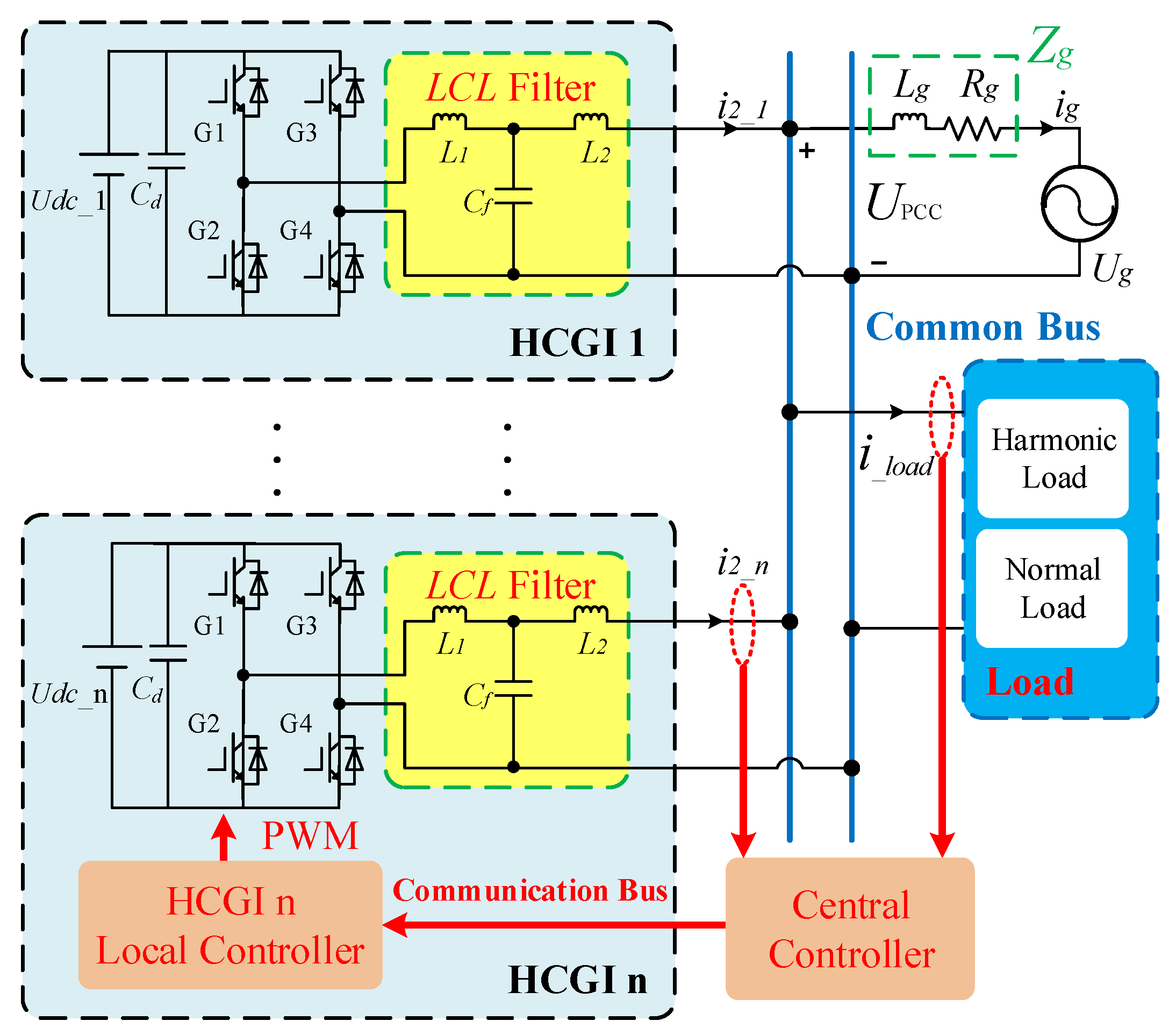
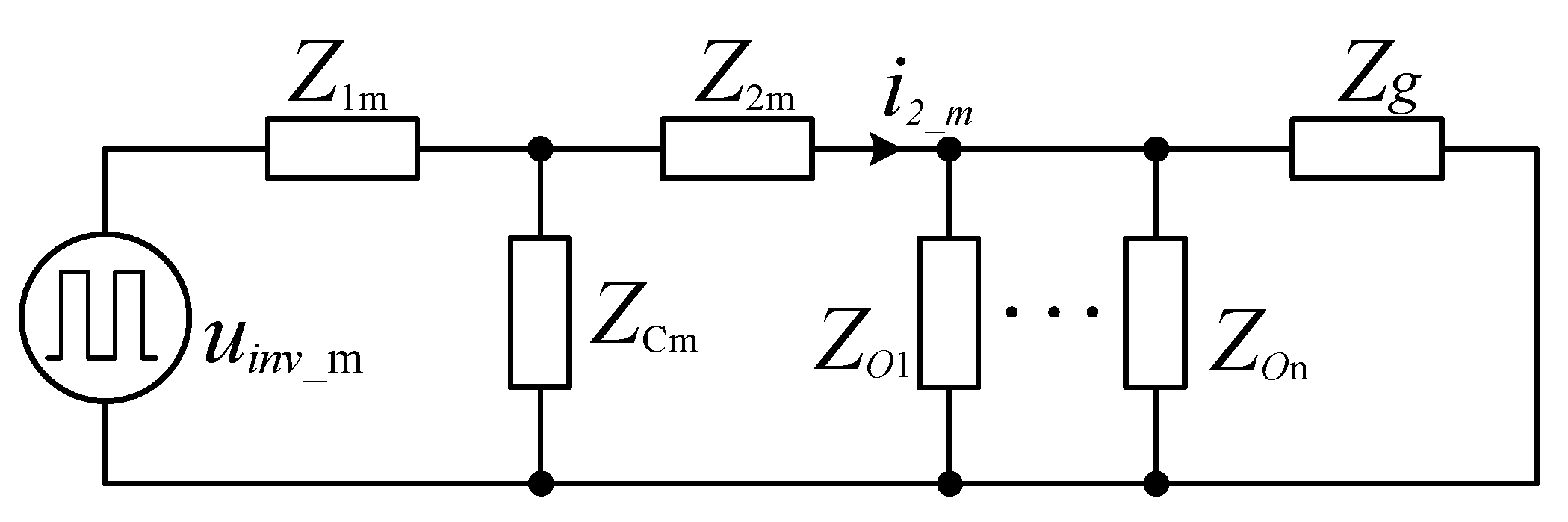
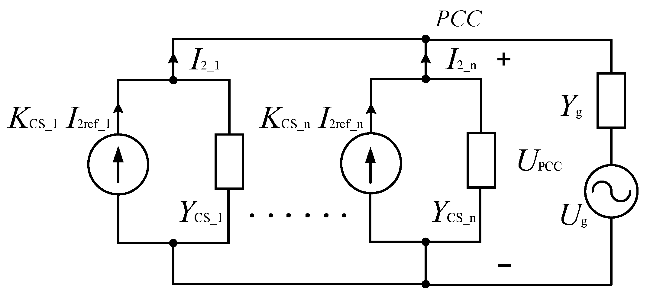
2.1. Analysis of Multi-Parallel HCGIs System

According to [23], the equivalent circuit of Figure 1 can be obtained and drawn in Figure 2, where $Z_{1\mathrm{m}}=s{L}_1$, $Z_{\mathrm{Cm}}=1/s{C}_f$, $Z_{2m}=s{L}_2$, $Z_g=s{L}_g+R_g$, and the Z_O1 and Z_On are calculated by:

$$\begin{array}{cc}{Z}_{oi}=Z_{1i}//Z_{Ci}+Z_{2i},& i=1,2,\cdots ,n\end{array}.$$

(1)

G_{o_m} is the system transfer function, which describes the relation between the inverter voltage u_{inv_m} and the output current i_{2_m} of the mth grid-connected inverter, and it can be expressed by:

$$G_{o\_m}=\frac{i_{2\_m}}{u_{inv\_m}}=\frac{Z_{Cm}}{Z_{eq3}(Z_{Cm}+Z_{eq2})},$$

(2)

where:

$$\{\begin{array}{l}{Z}_{eq1}=Z_{O1}//\cdots //Z_{Oi}//\cdots //Z_{On}(i\ne m)\\ Z_{eq2}=Z_{eq1}//Z_g+Z_{2m}\\ Z_{eq3}=Z_{eq1}//Z_{Ci}+Z_{1m}\end{array}.$$

(3)

In order to intuitively analyze the interaction of multi-parallel HCGIs, all parameters of HCGIs are selected to be the same in this paper. The parameters can be found in

Table 1. Parameters of the HCGIs system.

Symbol	Value	Symbol	Value
L1/mH	3	Ug/V	220
Cf/μF	10	Udc/V	400
L2/mH	2	Rg/Ω	0.2
Lg/mH	1.2	fs/kHz	20

, and Bode diagram of G_{o_m} with n grid-connected inverters is shown in Figure 3. It is obviously that there are additional resonance and anti-resonance peaks in the diagram. Specifically, with the increase of n, the position of the higher frequency resonance point remains unchanged, while the lower frequency resonance point shifts to the lower frequency band.

In order to improve the harmonic current compensation of HCGI in the multi-parallel situation, quasi-PR controllers are introduced into the current control loop, and the block diagram of the output current control loop for HCGI is shown in Figure 4.

According to Figure 4, the transfer function from the reference current i_{_ref} and the grid side voltage U_pcc to the output current i₂ for the mth HCGI is:

$$I_2{}_{\_m}(s)=K_{CS\_m}(s)I_{2\mathrm{ref}\_\mathrm{m}}(s)-Y_{CS\_m}(s)U_{\mathrm{pcc}}(s).$$

(4)

Based on the Norton equivalent circuit, the equivalent controlled source coefficient K_{CS_m} and the equivalent parallel admittance Y_{CS_m} are derived as:

$$K_{CS\_m}(s)=\frac{I_{2\_m}(s)}{I_{2\mathrm{ref}\_\mathrm{m}}(s)}=\frac{K_{\mathrm{PWM}}{G}_{\mathrm{PR}}{G}_{L1}{G}_C{G}_{L2}}{1+G_{L1}{G}_{L2}+G_C{G}_{L2}+K_{\mathrm{PWM}}{G}_{\mathrm{PR}}{G}_{L1}{G}_C{G}_{L2}},$$

(5)

$$Y_{CS\_m}(s)=\frac{I_{2\_m}(s)}{U_{pcc}(s)}=\frac{G_{L2}(1+G_{L1}{G}_C)}{1+G_{L1}{G}_{L2}+G_C{G}_{L2}+K_{\mathrm{PWM}}{G}_{\mathrm{PR}}{G}_{L1}{G}_C{G}_{L2}}.$$

(6)

where the K_PWM is pulse width modulation (PWM) gain of HCGI, $G_{L1}=1/s{L}_1$, $G_{\mathrm{c}}=1/s{C}_f$, $G_{L2}=1/s{L}_2$, and G_PR is the quasi PR controller represented as:

$$k\mathrm{p}+{\displaystyle \sum _{h=1,3,5\dots h\max }\frac{2k_{i,h}{\omega }_{c}s}{s^2+2{\omega }_{c}s+{(h{\omega }_n)}^2}}.$$

(7)

Equation (7) is the superposition of multiple PR controllers, so that the PR controller can track multiple harmonics at the same time. k_p is the proportional coefficient, ${\omega }_c$ is the cut-off frequency, ${\omega }_{\mathrm{n}}$ is the fundamental frequency, h is the order of harmonics, and k_i,h is the hth harmonic resonance gain.

The Norton equivalent circuit of multi-parallel HCGIs is shown in Figure 5. According to [24], the influence of the grid-side reference current I_{2ref_m} on the grid-side current I_{2_m} of the mth HCGI in multiple situation is:

$${\mathsf{\Phi }}_{O\_m}=K_{CS\_m}-\frac{Y_{CS\_m}{K}_{CS\_m}}{{\displaystyle \sum _{i=1}^n{Y}_{CS\_i}+Y_g}}.$$

(8)

In order to clearly observe the effect of multi-parallel connection on the resonance points, the maximum order h_max of (7) for PR controller is set to 1 in Figure 6. Figure 6 shows Bode diagram of the Φ_{O_m} with different n. Same as the analysis results of system transfer function G_{o_m}, when the number of resonance points for HCGIs system changes from 1 to 2, one resonance point is fixed, and the new resonance point is unfixed. As the number of HCGIs n increases, the frequency of new resonance point shifts to the lower frequency and the peak value of the new resonance point decreases.

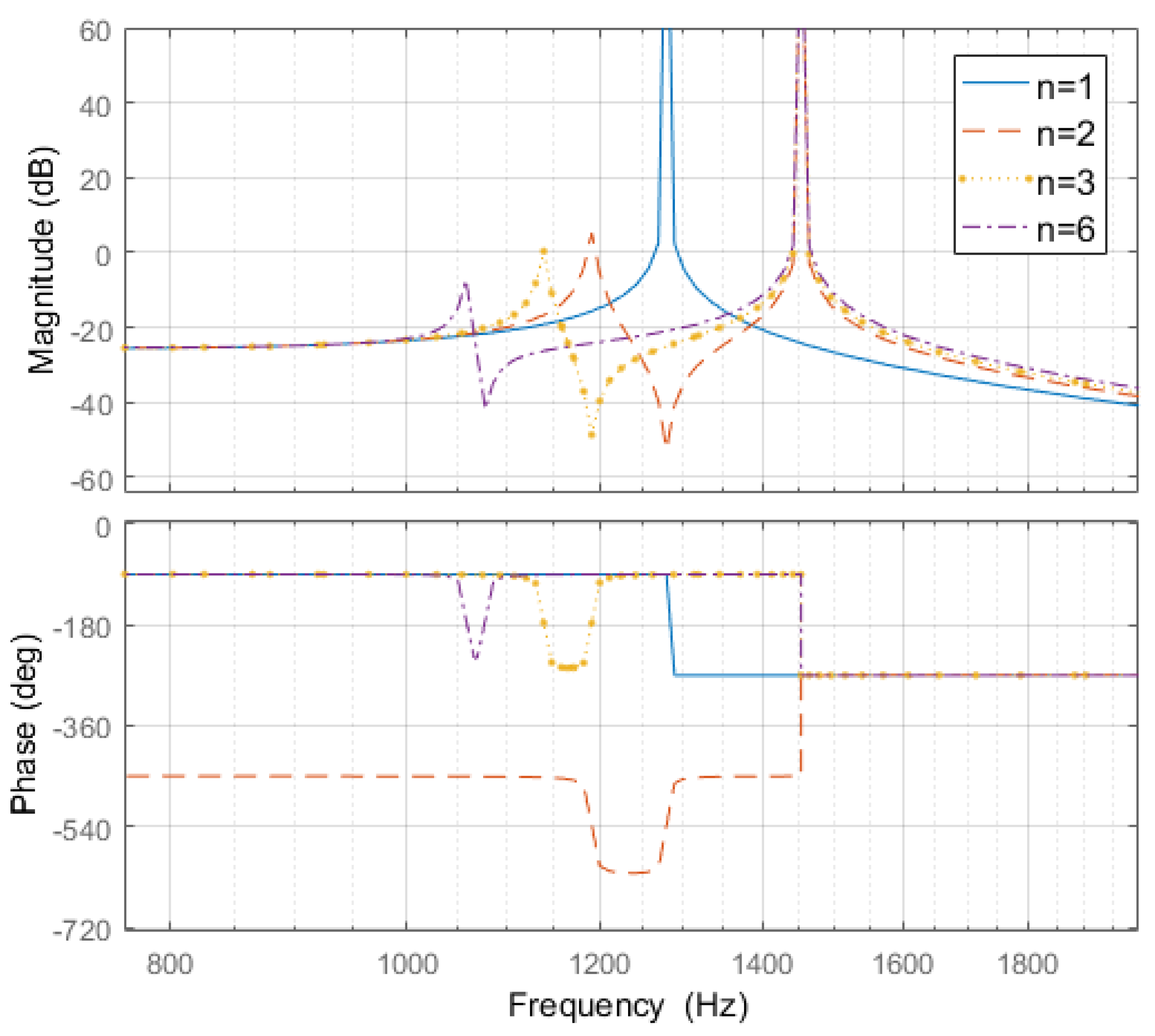
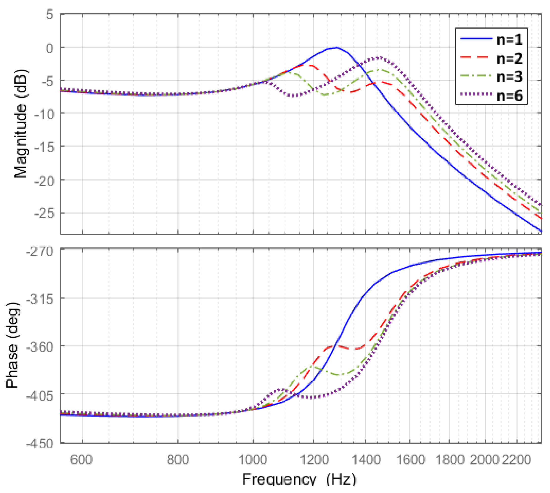
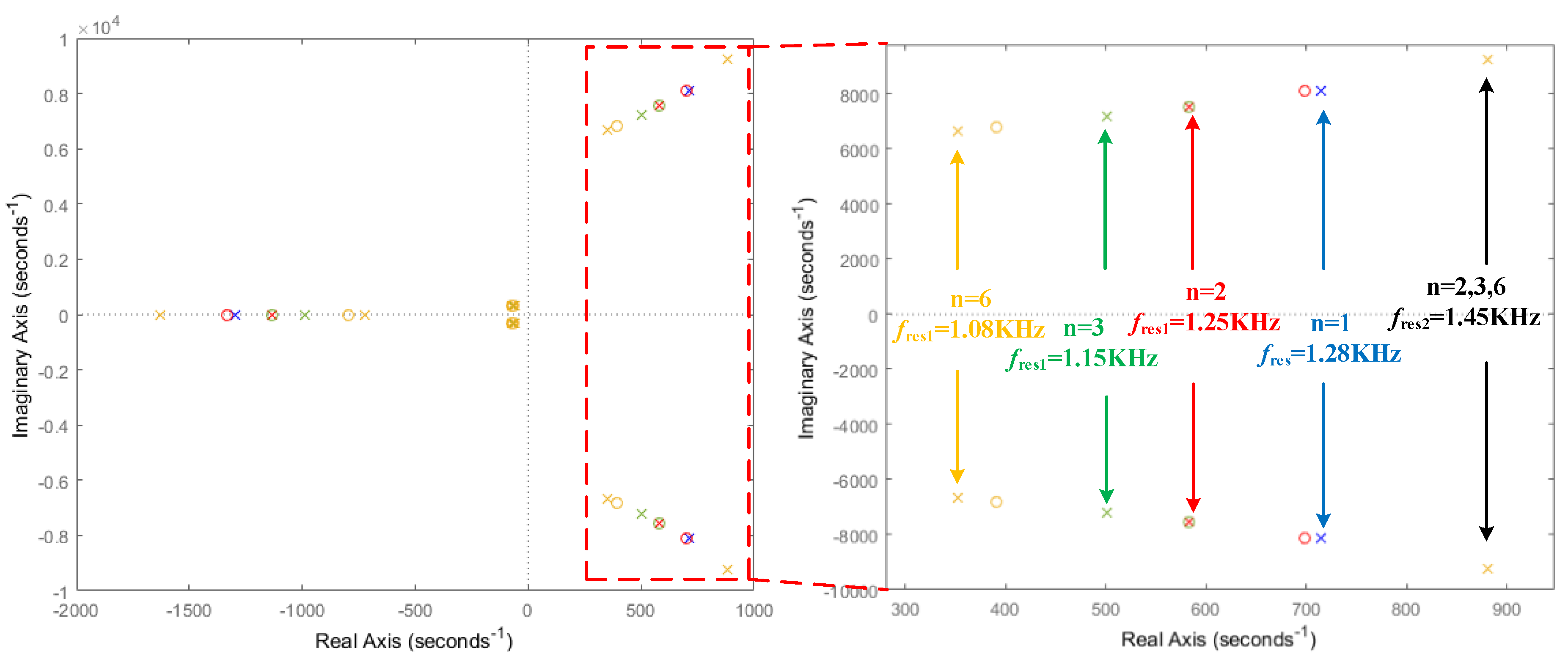
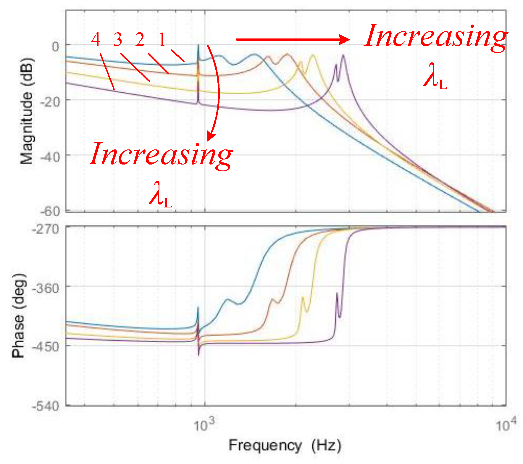
2.2. Influence of Multi-Parallel Inverters on Control Bandwidth

Furthermore, to analyze the influence of the new resonance points on bandwidth, the zero-pole diagrams of single HCGI and multi-parallel HCGIs system are shown in Figure 7. Table 1 shows the relationship between the number of HCGIs n and the resonant frequencies. There is one pair of poles on the right side of the imaginary axis in the single HCGI system, which means the system would be unstable at this frequency. A new pair of poles appears on the right side of the imaginary axis, which corresponds to the new resonant point of multi-parallel HCGIs system.

The common harmonic frequencies of single phase are 3rd, 5th, 7th, 9th and 11th order, and higher harmonic frequencies can be 17th, 19th, even 23th, 25th order [29]. As shown in Figure 7 and

Table 2. The relationship between n and the resonant frequencies.

n	1	2	3	6
fres1 (Hz)	/	1251	1149	1082
fres2 (Hz)	1279	1453	1453	1453

, the frequency of the new resonance point would be less than 1250 Hz (25th order harmonic), which may affect system stability and decrease the control bandwidth. In this context, it is necessary to propose a method to solve the bandwidth issue in multi-parallel HCGIs systems.

3. Bandwidth Control of Multi-parallel HCGIs System

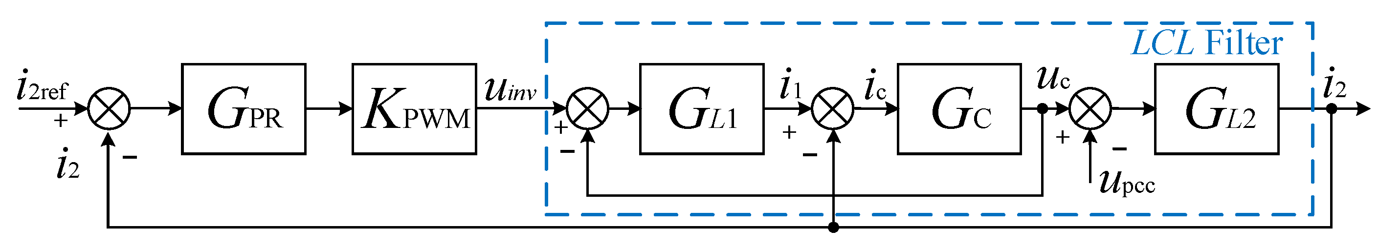
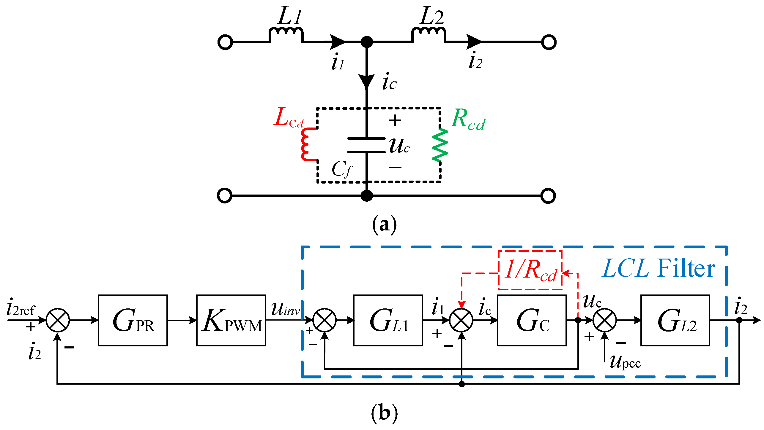
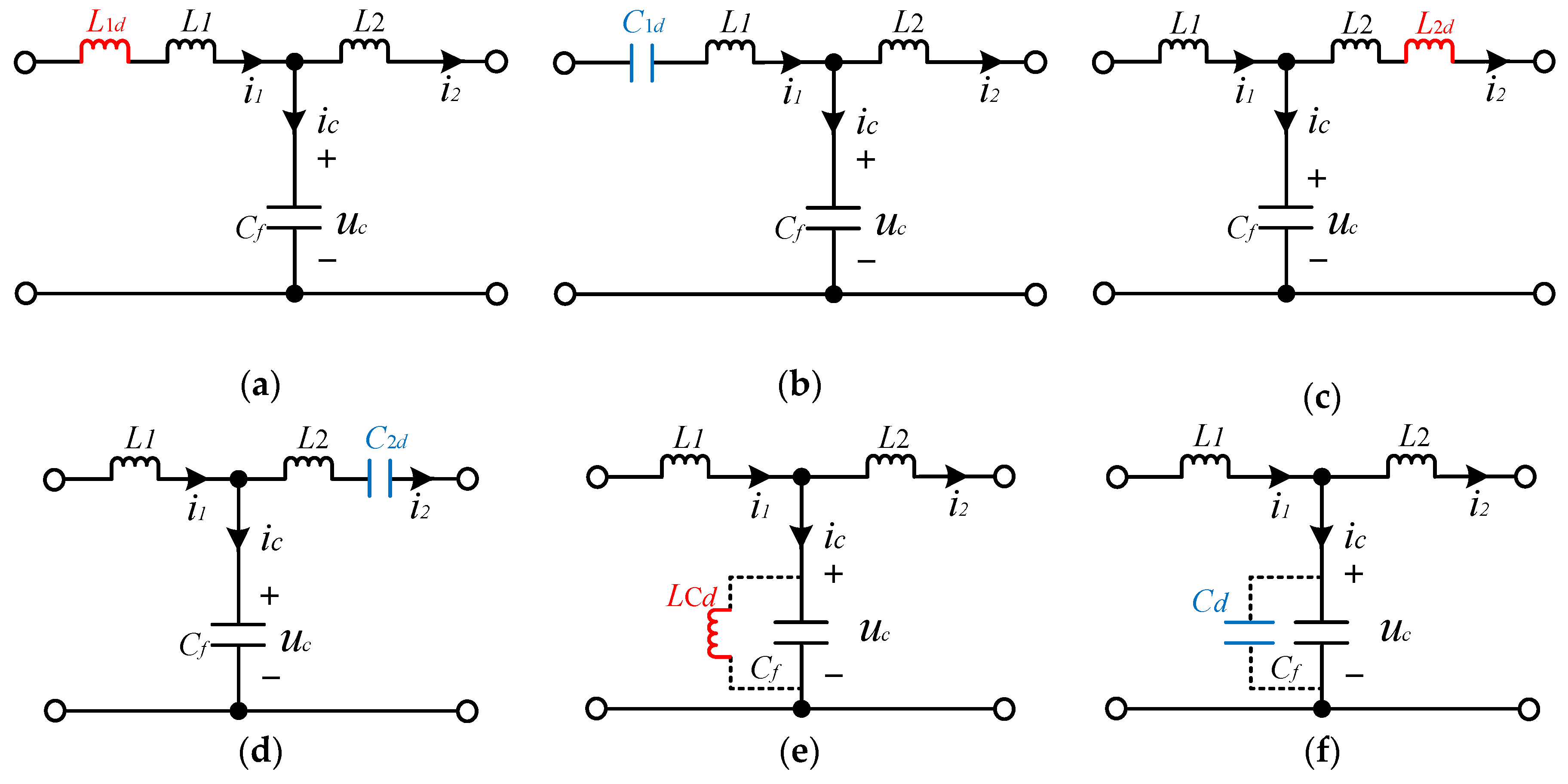
3.1. Active Damping Method in Multi-Parallel HCGIs System

As previously analyzed in Section 2, the new resonant point is the cause of the bandwidth issue in multi-parallel HCGIs system. In a general situation, the active damping method is used to suppress the resonance peak of grid-connected inverters. According to [32], active damping methods can be classified into two kinds: one is the notch-filter-based active damping, and the other is the state-variable-feedback active damping.

In view of the notch-filter-based active damping method, the notch filter may not match the resonance frequencies exactly, as there are uncertainties of resonant frequencies in multi-parallel HCGIs system. Thus, the performance of notch-filter-based active damping may worsen or even be ineffective.

As for the state-variable-feedback active damping method, it uses the feedback of proper state variable to mimic a virtual resistor in place of the physical one, and it has been widely used in the practical application. According to [32], the resistor in parallel with the capacitor shows the best damping performance, and the function-equivalent active-damping solution can be derived as follows. The LCL filter equivalent circuit and control block diagram of HCGI using a virtual resistor R_cd in parallel with capacitor are shown in Figure 8.

Bode diagrams of the system with different R_cd are shown in Figure 9a, and the ones with harmonic current compensation are presented in Figure 9b.

As shown in Figure 9a, two resonance peaks can be effectively suppressed by virtual resistance. Furthermore, with the decreasing resistance of R_cd (from 1 to 4), the Bode diagram of the system will steepen continuously in the high-frequency band. Figure 9b shows that suppressing resonance peak will affect the high-frequency harmonic current compensation, and the effect becomes noticeable as the harmonic frequency approaches the resonance frequency. In this context, the bandwidth issue appears, which is addressed by the method proposed in the next section.

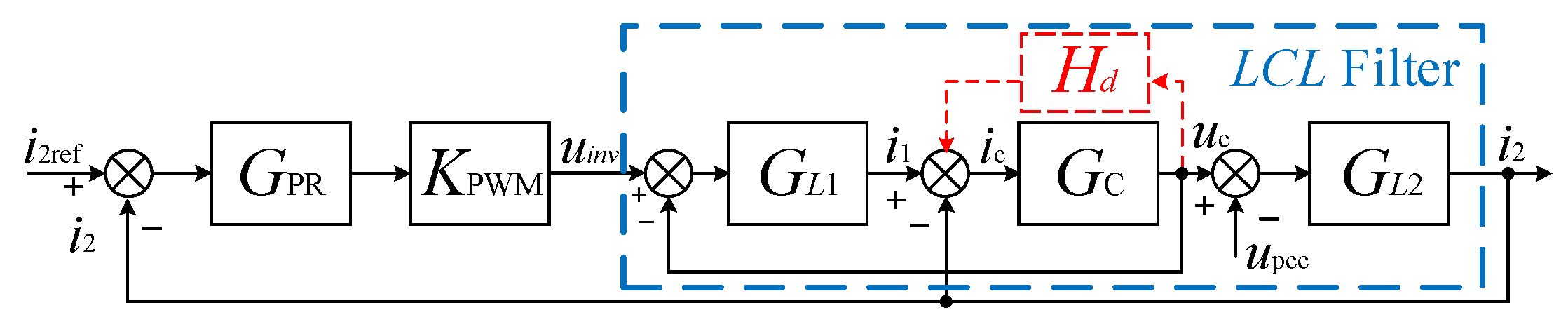
3.2. Virtual Impedance Method for the Bandwidth Control

By observing Equations (1)–(3), the Z_1m, Z_2m and Z_Cm would affect the resonant frequencies of the system. Motivated by this observation, the virtual impedance method is proposed in this study.

Based on reference [33], there are six kinds of virtual impedance equivalent circuits which can provide damping on L₁, L₂ and C_f using voltage and current feedback signals on L₁, L₂ and C_f. Considering the concerned bandwidth issue, these six equivalent circuits shown in Figure 10 need to be analyzed and the most effective method for increasing the control bandwidth identified. To do that, the influences of different virtual impedance circuits on the resonant frequency of LCL filter are analyzed and compared. According to the analysis results of Section 2, the analysis of the model without considering control can reflect resonance points characteristics in multi-parallel situation, so the influence of six kinds of virtual impedance on the system transfer function G_{o_m} of mth HCGI is compared for simplicity.

Based on Figure 10a,b, the Z_1m with virtual inductance L_1d and virtual capacitors C_1d can be rewritten as:

$$\begin{array}{l}{Z}_{1\mathrm{m}\_\mathrm{L}1\mathrm{d}}=s(L_1+L_{1d})\\ Z_{1\mathrm{m}\_\mathrm{C}1\mathrm{d}}=s{L}_1+\frac{1}{s{C}_{1d}}\end{array}$$

(9)

Based on Figure 10c,d, the Z_2m with virtual inductance L_2d and virtual capacitors C_2d can be rewritten as:

$$\begin{array}{l}{Z}_{2\mathrm{m}\_\mathrm{L}2\mathrm{d}}=s(L_2+L_{2d})\\ Z_{2\mathrm{m}\_\mathrm{C}2\mathrm{d}}=s{L}_2+\frac{1}{s{C}_{2d}}\end{array}$$

(10)

Based on Figure 10e,f, the Z_Cm with virtual inductance L_Cd and virtual capacitors C_d can be rewritten as:

$$\begin{array}{l}{Z}_{\mathrm{Cm}\_\mathrm{Lcd}}=\frac{s{L}_{Cd}}{s^2{L}_{Cd}{C}_f+1}\\ Z_{\mathrm{Cm}\_\mathrm{Cd}}=\frac{1}{s(C_d+C_f)}\end{array}$$

(11)

By substituting Equations (9)–(11) into Equations (1)–(3), and the values of the six kinds of virtual impedance are shown in

Table 3. Parameters of virtual impedance.

Symbol	Value	Symbol	Value
L1d/mH	1.5	C1d/μF	10
L2d/mH	1	C2d/μF	10
Lcd/mH	1.5	Cd/μF	10

, the bode diagrams for system transfer function G_{o_m} of mth HCGI with 6 kinds of virtual impedance are shown in Figure 11.

As observed from Figure 11a,c,f, the resonance frequencies of G_{o_m} decrease with the equivalent inductances L_1d, L_2d connected in series and virtual capacitors C_d connected in parallel, while from Figure 11b,d, there are two new resonance pecks with virtual capacitors C_1d and C_2d. By comparison, Figure 11e shows that the resonance frequencies increase with the virtual inductance L_cd. Therefore, the virtual inductance L_cd can shift right the resonant frequencies, which may effectively solve the bandwidth issue of HCGIs systems.

3.3. Analysis of Bandwidth Control

In order to check the effectiveness of virtual inductance L_cd in multi-parallel HCGIs system, its representation of HCGI output current loop is given in Figure 12, where virtual feedback channel H_d = 1/sL_cd represents the virtual inductance L_cd paralleled on capacitance C_f, and the LCL filter equivalent circuit is shown in Figure 10e.

According to Figure 12, the equivalent controlled source coefficient and equivalent shunt admittance of HCGI with virtual inductance are obtained as:

$$K_{CS\_d}(s)=\frac{K_{\mathrm{PWM}}{G}_{\mathrm{PR}}{G}_{L1}{G}_C{G}_{L2}}{1+H_d{G}_C+G_{L1}{G}_{L2}+G_C{G}_{L2}+K_{\mathrm{PWM}}{G}_{\mathrm{PR}}{G}_{L1}{G}_C{G}_{L2}},$$

(12)

$$Y_{CS\_d}(s)=\frac{G_2(1+H_d{G}_c+G_{L1}{G}_C)}{1+H_d{G}_C+G_{L1}{G}_{L2}+G_C{G}_{L2}+K_{\mathrm{PWM}}{G}_{\mathrm{PR}}{G}_{L1}{G}_C{G}_{L2}}.$$

(13)

where H_d = 1/sL_cd, according to Equations (8), (12) and (13), the Φ_{O_d} of the multi-parallel HCGIs system with the virtual inductance is rewritten as:

$${\mathsf{\Phi }}_{O\_d}=K_{CS\_d}-\frac{Y_{CS\_d}{K}_{CS\_d}}{{\displaystyle \sum _{i=1}^n{Y}_{CS\_d}+Y_g}}.$$

(14)

To illustrate that the virtual inductance method could shift right resonance frequencies of multi-parallel HCGIs, Bode diagrams of Φ_{O_d} with $L_{cd}=L_1/2$ in 3-parallel and 5-parallel HCGIs are shown in Figure 13. It is clearly seen that the virtual parallel-inductance L_cd can solve the issue of bandwidth reduction in the multi-parallel HCGIs system by shifting the resonance frequency.

Thus, the bandwidth control method with virtual resistance and virtual inductance is proposed, and the equivalent circuit is shown in Figure 14.

Based on Figure 14, virtual feedback channel H_d shown in Figure 10 can represent the virtual impedance and can be rewritten as:

$$H_d=H_{Rd}+H_{Lcd},$$

(15)

where $H_{Lcd}=1/s{L}_{cd}$ represents virtual inductance L_cd, and $H_{Rd}=1/R_{cd}$ represents virtual resistance R_cd.

3.4. Design of Feedback Channel G_d

3.4.1. Feedback channel comparison

According to [34], the virtual resistance paralleled on capacitance C_f can be realized by feedback of capacitor current and capacitor voltage. Accordingly, the virtual feedback channel H_d can be realized by feeding-back of the capacitor current and capacitor voltage. As shown in Figure 15a,b, the real feedback channel is expressed as G_d.

According to Figure 15, the comparison between the feedback signals for virtual impedance is summarized in

Table 4. The feedback signal comparison for virtual impedance.

Feedback Signal	uc	ic
$G_d$	$\frac{s{L}_1}{K_{\mathrm{PWM}}{R}_{cd}}+\frac{L_1}{K_{\mathrm{PWM}}{L}_{cd}}$	$\frac{L_1}{K_{PWM}{C}_f{R}_{cd}}+\frac{L_1}{s{K}_{\mathrm{PWM}}{C}_f{L}_{cd}}$

. Where, the capacitor voltage feedback consists of a constant and a differential link, and the capacitor current feedback consists of a constant and an integral link. In engineering implementation, integral feedback is more difficult than differential feedback, and it is difficult to detect capacitor current because of many high-frequency disturbances to detect. Consequently, the virtual impedance feeding-back by capacitor voltage u_c is used in this paper.

In Table 4, the feedback channel G_d with capacitor voltage u_c feedback can be written as:

$$G_d=\frac{s{L}_1}{K_{\mathrm{PWM}}{R}_{cd}}+\frac{L_1}{K_{\mathrm{PWM}}{L}_{cd}}=s{\lambda }_R+{\lambda }_L$$

(16)

where ${\lambda }_R$ is the feedback factor of virtual resistance, and ${\lambda }_L$ is the feedback factor of virtual inductance.

3.4.2. Design of the Feedback Constant

For the proposed method, the two feedback constants ${\lambda }_R$ and ${\lambda }_L$ need to be designed by the three expectations including increasing system bandwidth, suppressing resonance peaks, and ensuring the performance of high-frequency harmonic current compensation. The design steps of feedback factors ${\lambda }_R$ and ${\lambda }_L$ are as follows:

Identify the expected values according to the expectation of bandwidth, resonance peak suppression and harmonics compensation for multiple HCGIs;

Determine the relationship between the expected values and the parameters of the proposed method, and obtain the range of the parameters by considering each expected value synthetically.

In this paper, the expected value of the bandwidth can be defined as the improved bandwidth frequency f_B. Meanwhile, the expected values of suppressing resonance peaks and ensuring high-frequency harmonic current compensation are described by system magnitude ${\left|{\mathsf{\Phi }}_{O\_d}\right|}_C$ and ${\left|{\mathsf{\Phi }}_{O\_d}\right|}_S$. Specifically, the magnitude of the system at harmonics frequency should be greater than ${\left|{\mathsf{\Phi }}_{O\_d}\right|}_C$ to ensure the performance of harmonic compensation, and the magnitude of the system at resonance frequencies should be smaller than ${\left|{\mathsf{\Phi }}_{O\_d}\right|}_S$ to ensure resonant peaks effectively suppressed.

According to Equation (16), the relationship between feedback constant ${\lambda }_R$ and virtual resistance is obtained as:

$${\lambda }_R=\frac{L_1}{K_{\mathrm{PWM}}{R}_{cd}}$$

(17)

For a given HCGI, the values of L₁ and K_PWM are fixed, so ${\lambda }_R$ is inversely proportional to R_cd. Therefore, the conclusion in Section 3.1 can be rewritten as follows: the introduction of ${\lambda }_R$ can effectively suppress the resonance peaks, and the suppression effect is gradually enhanced with the increase of ${\lambda }_R$. However, the effect of current compensation decreases while enhancing the suppression effect gradually.

As for the feedback constant ${\lambda }_L$, the feedback channel is $G_d={\lambda }_L$ only with virtual inductance, and H_d can be formulated by:

$$H_d=\frac{K_{PWM}}{s{L}_1}{\lambda }_L$$

(18)

By substituting Equation (18) into Equations (12)–(14), Bode diagram of Φ_{O_d} with virtual inductance L_cd is drawn in Figure 16.

For an intuitive description, this paper takes the amplitude of 19th order harmonic current as an example. As shown in Figure 16, with the increase of ${\lambda }_L$ (from 1 to 4), the resonance peaks can be shifted to the right continuously. In addition, the right shift of the resonant peaks will also be accompanied by the overall decline of the high-frequency band. For an intuitive description, the relationships between ${\lambda }_R$, ${\lambda }_L$ and the three expected directions are listed in

Table 5. The relationships between ${\lambda }_R$, ${\lambda }_L$ and the three expected directions.

Expected Direction	$\mathbf{Increasing} {\mathit{\lambda }}_{\mathit{L}}$	$\mathbf{Increasing} {\mathit{\lambda }}_{\mathit{R}}$
Bandwidth improvement (Resonance peaks shift right)	↑	-
Resonance peaks suppression	-	↑
High-frequency harmonics compensation effect	↓	↓

.

In this paper, the expected improved bandwidth frequency f_B is 1250 Hz (25th order harmonic) which is the highest harmonic current frequency of a single HCGI system. According to references [10,11,12,13,14,15,16], if K_{O_d} is greater than 0.5 at high frequency section, the performance of harmonic compensation is acceptable. Besides, according to references [17,18,19,20,21], if the system gain K_{O_d} smaller than 0.2, the resonant peak can be effectively suppressed.

The gain of system K_{O_d} can be obtained as:

$$K_{O\_d}=20\lg \left|{\mathsf{\Phi }}_{O\_d}\right|$$

(19)

By substituting K_{O_dc} = 0.5 and K_{O_dc} = 0.2 into Equation (19), ${\left|{\mathsf{\Phi }}_{O\_d}\right|}_C$ is −6.02 and ${\left|{\mathsf{\Phi }}_{O\_d}\right|}_S$ is −13.98. With virtual resistance and virtual inductance, H_d is rewritten as (20):

$$H_d=\frac{K_{PWM}}{L_1}{\lambda }_R+\frac{K_{PWM}}{s{L}_1}{\lambda }_L$$

(20)

By substituting Equation (20) into Equations (12)–(14), the critical values of ${\lambda }_L$ and ${\lambda }_R$ are calculated and shown in

Table 6. The range of λ_L and λ_R.

Expectation	${\mathit{\lambda }}_{\mathit{R}}$	${\mathit{\lambda }}_{\mathit{L}}$	$1+{\mathit{\lambda }}_{\mathit{R}}$
Bandwidth improvement (fres > fB)	-	>0.48	-
Resonance peaks suppression ($\left|{\mathsf{\Phi }}_{O\_d\_res1}\right|$ < ${\left|{\mathsf{\Phi }}_{O\_d}\right|}_S$, $\left|{\mathsf{\Phi }}_{O\_d\_res2}\right|$ < ${\left|{\mathsf{\Phi }}_{O\_d}\right|}_S$)	>2.2 × 10−4	-	>1 + 0.83 × 10−4
The 19th and 25th order harmonics compensation effect ($\left|{\mathsf{\Phi }}_{O\_d\_19th}\right|$ > ${\left|{\mathsf{\Phi }}_{O\_d}\right|}_C$, $\left|{\mathsf{\Phi }}_{O\_d\_25th}\right|$ > ${\left|{\mathsf{\Phi }}_{O\_d}\right|}_C$)	<1.4 × 10−4	<1.63	<1 + 1.12 × 10−4

. ${\lambda }_R$ should be larger than 2.2 × 10⁻⁴ to maintain the suppression effect while smaller than 1.4 × 10⁻⁴ to ensure harmonics compensation. Thus, it is difficult to use virtual resistance alone to ensure high-frequency harmonics current compensation and suppression effect together.

Because ${\lambda }_R$ does not affect bandwidth improvement by ${\lambda }_L$, it is better to design ${\lambda }_L$ first. Considering the expectations of high-frequency harmonics compensation effect and the bandwidth improvement, ${\lambda }_L$ is set as 1. Moreover, when ${\lambda }_L$ = 1, the critical values of ${\lambda }_R$ considering the expectations of high-frequency harmonics compensation effect and resonance peak suppression effect are also calculated and shown in Table 6.

Considering a tradeoff between high-frequency harmonics compensation and resonant peaks suppression, ${\lambda }_L$ is 1 and ${\lambda }_R$ is 10⁻⁴ for 3-parallel HCGIs system in this paper. Accordingly, the feedback channel G_d is written as:

$$G_d={10}^{-4}s+1.$$

(21)

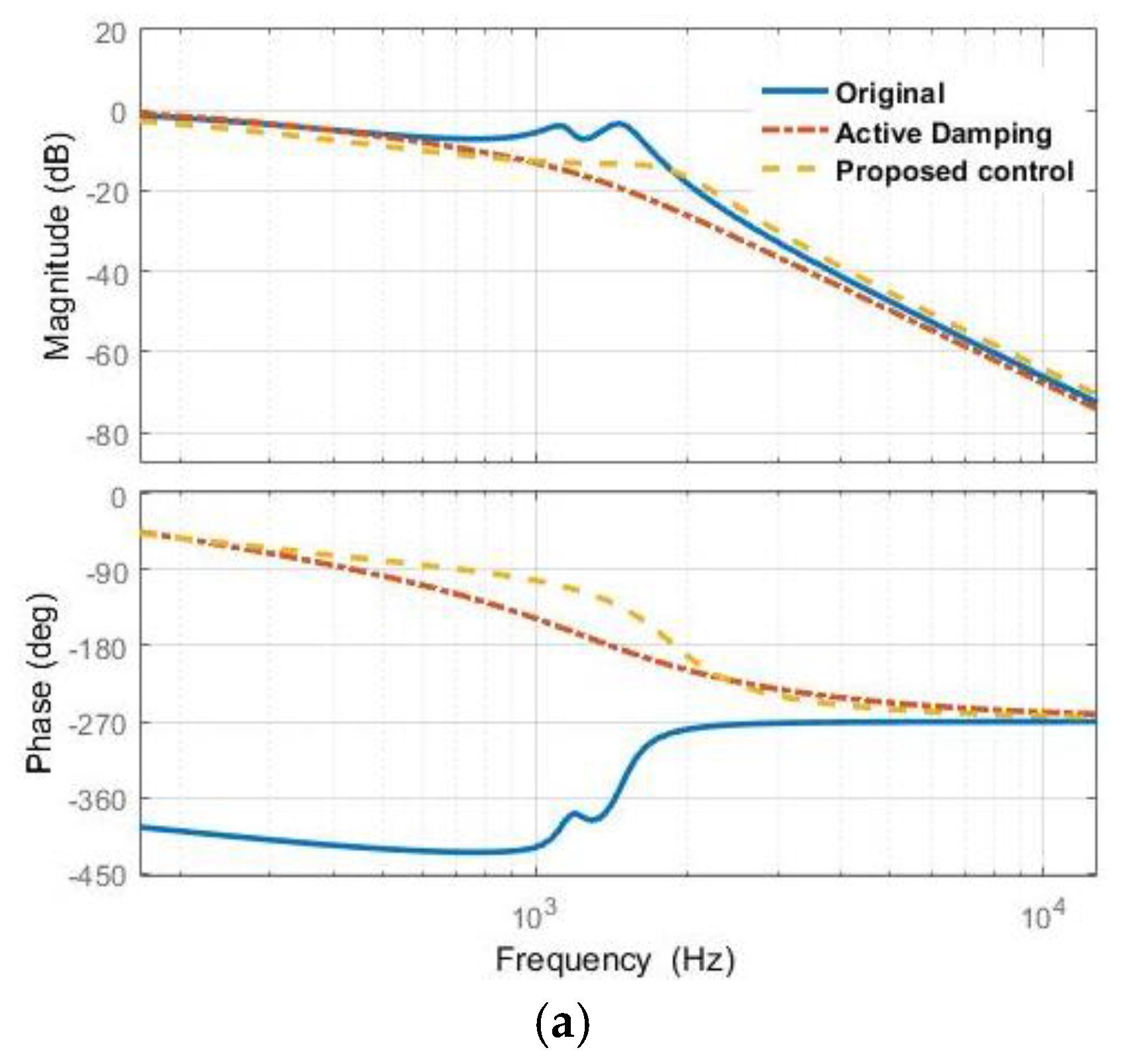
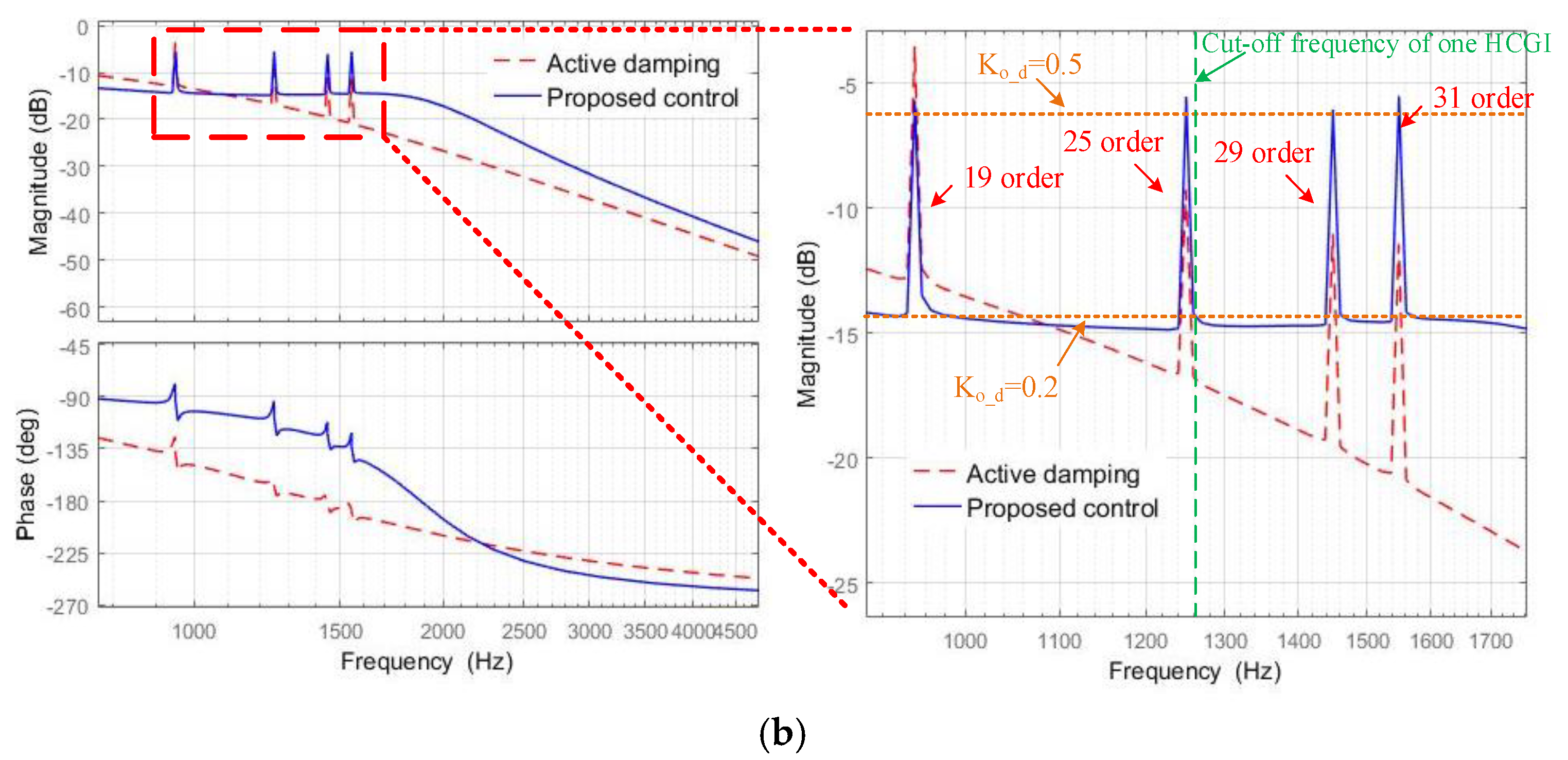
3.4.3. Comparison of Performance between the Proposed Control and Active Damping

Figure 17 shows Bode diagram of 3-parallel HCGIs system with two methods. The proposed control method use the parameters designed in Section 3.4.2, and active damping method uses the parameters which provide the same expectation of resonance peaks suppression.

Figure 17a shows the system Bode diagram of HCGI with controller only for fundamental current tracking, which intuitively illustrates the effect of proposed control and the active damping methods. Under the same suppression effect at the original new resonance frequency, the value of ${\lambda }_R$ in the proposed method is smaller than that in the active damping method, which means that it has a less influence on high-frequency harmonics compensation.

Figure 17b shows the high-frequency harmonic current compensation and bandwidth improvement of HCGI, where the 19th, 25th, 29th and 31th order harmonics are presented. It is clearly shown that the compensation effect is further ensured by shifting the resonant peak away from the compensated harmonic frequency. By comparison with the active damping method, the proposed control has a much better compensation effect on the 25th order harmonics and it can compensate some harmonics with even higher frequency than the bandwidth of a single HCGI. Thus, it is concluded that the proposed control can improve the bandwidth of HCGI system with effective resonant peaks suppression and good harmonic compensation.

4. Result Validation

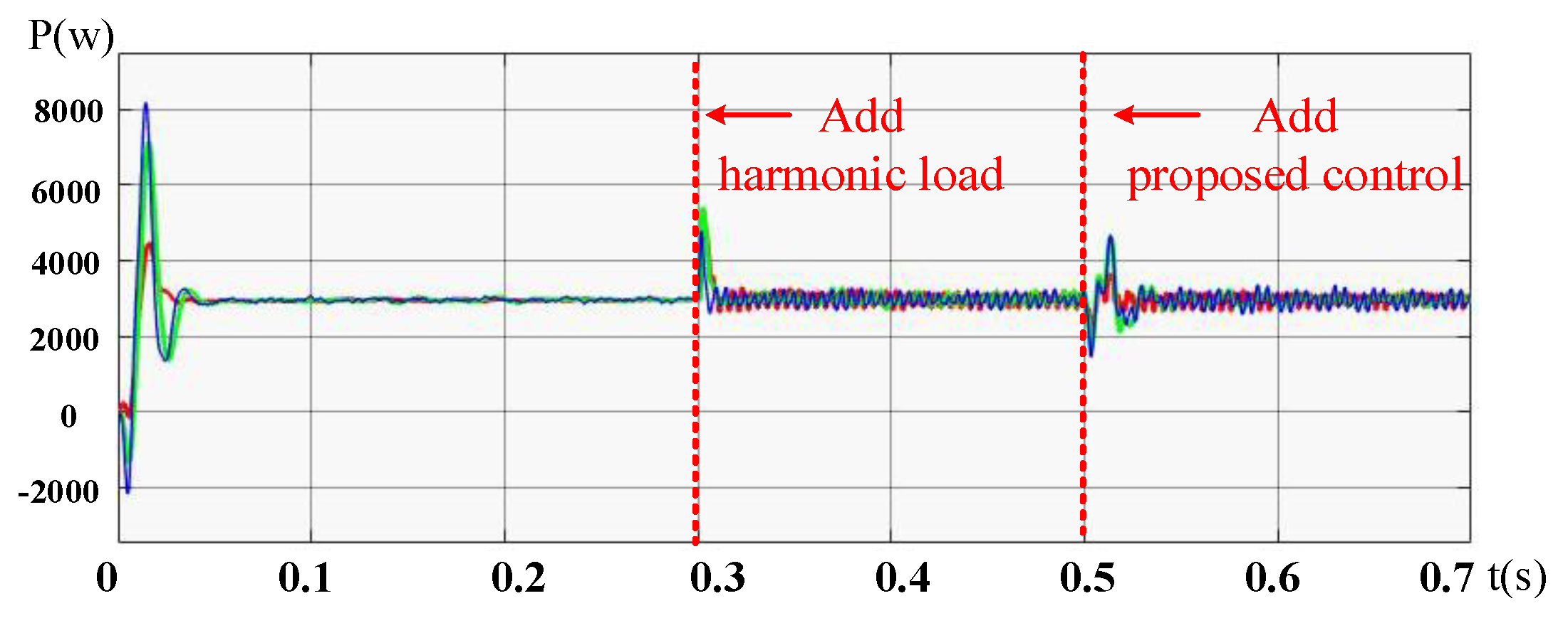
4.1. Simulation Validation

In order to verify the correctness of the proposed bandwidth control method, a 3-parallell- HCGI-based system is established in the MATLAB/Simulink platform (MATLAB2016a), and the parameters of this system are listed in Table 1. Two simulations are presented: one case gives the influence of the proposed bandwidth control method for low-frequency harmonic compensation, and the other shows results of high-frequency harmonic compensation and control bandwidth.

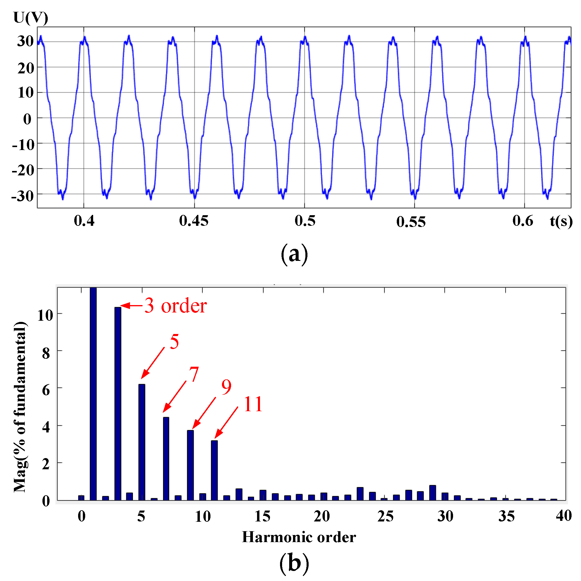
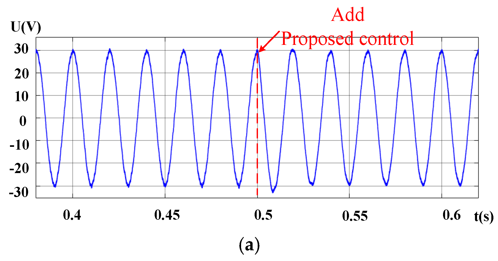
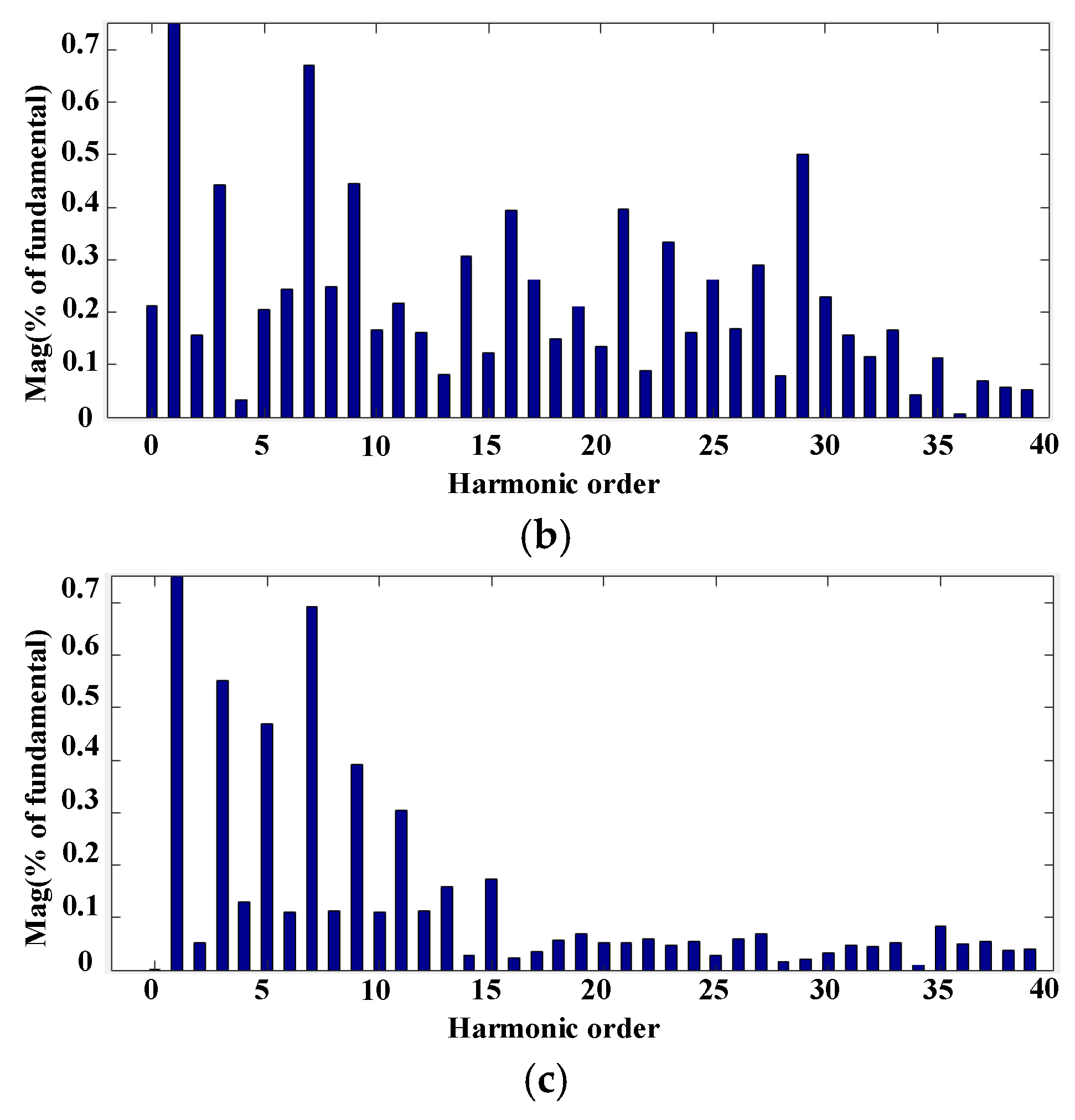
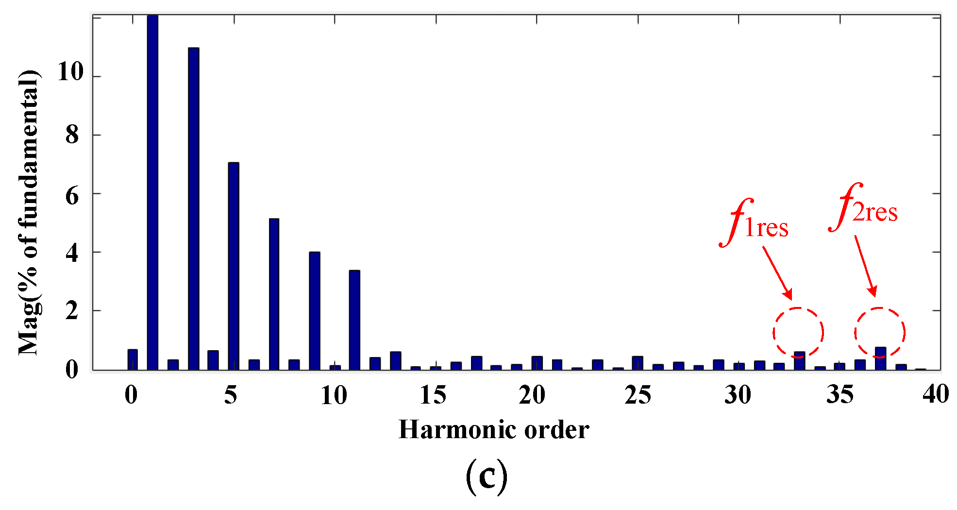
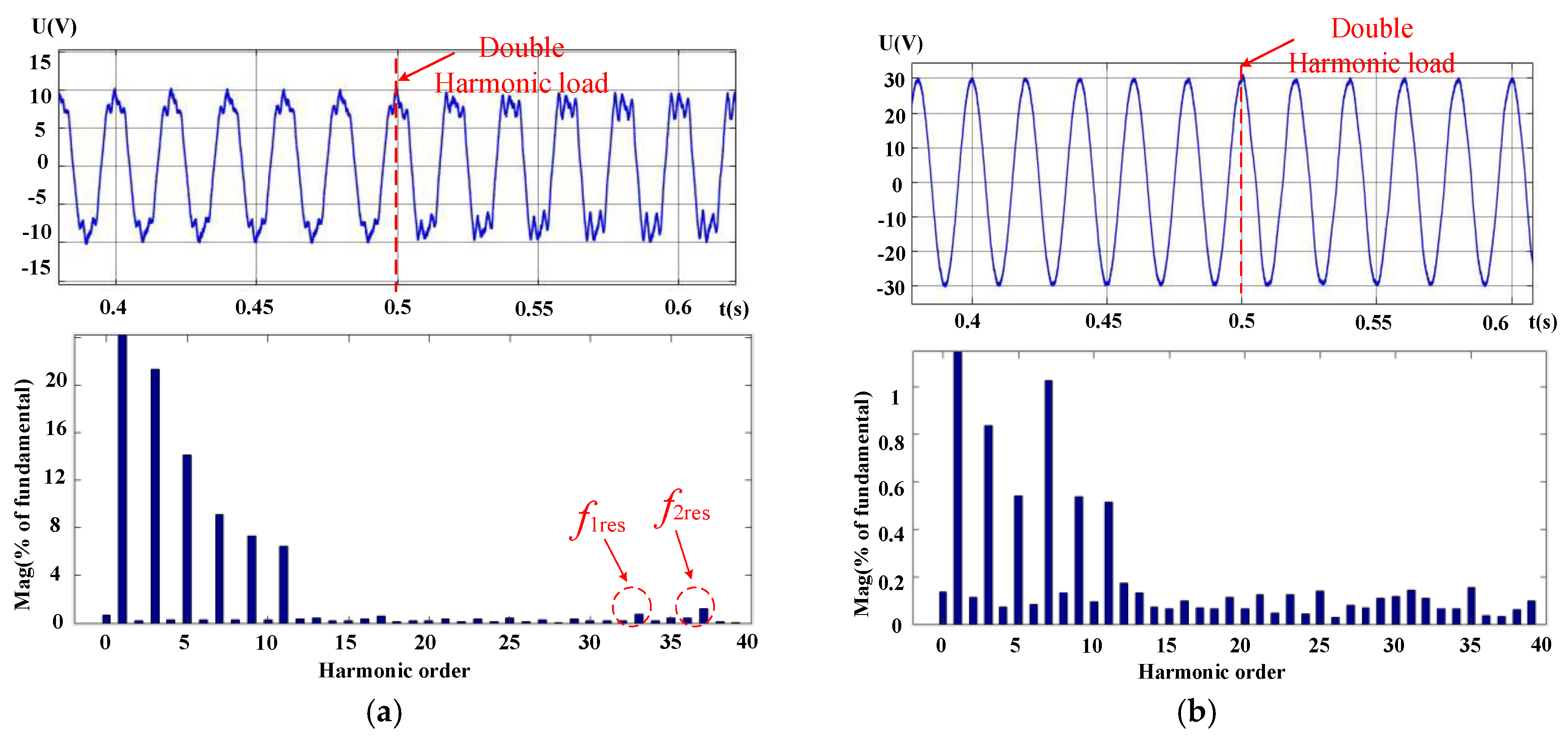
4.1.1. Low-order Harmonic Results

In this case, there are three HCGIs paralleled with a harmonic source, while each HCGI output the Root Mean Square (RMS) of the fundamental current is 7.07 A. The performance of power output in the three HCGIs system is shown in the Figure 18. Before t = 0.3 s, the three HCGIs work as generic inverters, the harmonic load is added at 0.3 s and the proposed control method is added at 0.5 s.

Figure 19 shows the grid current and its Total Harmonic Distortion (THD) analysis in the three HCGIs system without harmonic compensation, from which it is seen that the grid current contains harmonic current of 3rd, 5th, 7th, 9th, 11th order and its THD is 13.91%.

The grid current and its THD analysis with harmonic compensation are shown in Figure 20, respectively. The THD of grid current is 2.15%, which means that the harmonic current in grid current has been effectively compensated. After t = 0.5 s, when the proposed control is added, the THD of grid current is 2.01%, which illustrates that the low frequency harmonic compensation is not affected by the proposed control method.

Figure 21 shows the output current and its THD analysis of one HCGI with harmonic compensation. Before t = 0.5 s, the system works without the proposed control method, while after t = 0.5 s, it works with the proposed method. As shown in Figure 21b, there are two resonant peaks of HCGI output current near 23th fundamental wave (1150 Hz) and 29th fundamental wave (1453 Hz). In Figure 21c, with the proposed method activated, the frequency of two resonance points shifts right and the harmonic contents of the resonant frequencies are reduced.

The output current of HCGI and grid current with variable harmonic load are shown in Figure 22. Before t = 0.5 s, the HCGIs work with the proposed bandwidth control method, after t = 0.5 s, the harmonic load is doubled. As shown in Figure 22a, the two resonant frequencies of HCGI output current are still shifted right. According to Figure 22b, the THD of grid current is 2.87% with the doubled harmonic load, which illustrates the low frequency harmonic compensation is guaranteed with the proposed control method in the dynamic situation.

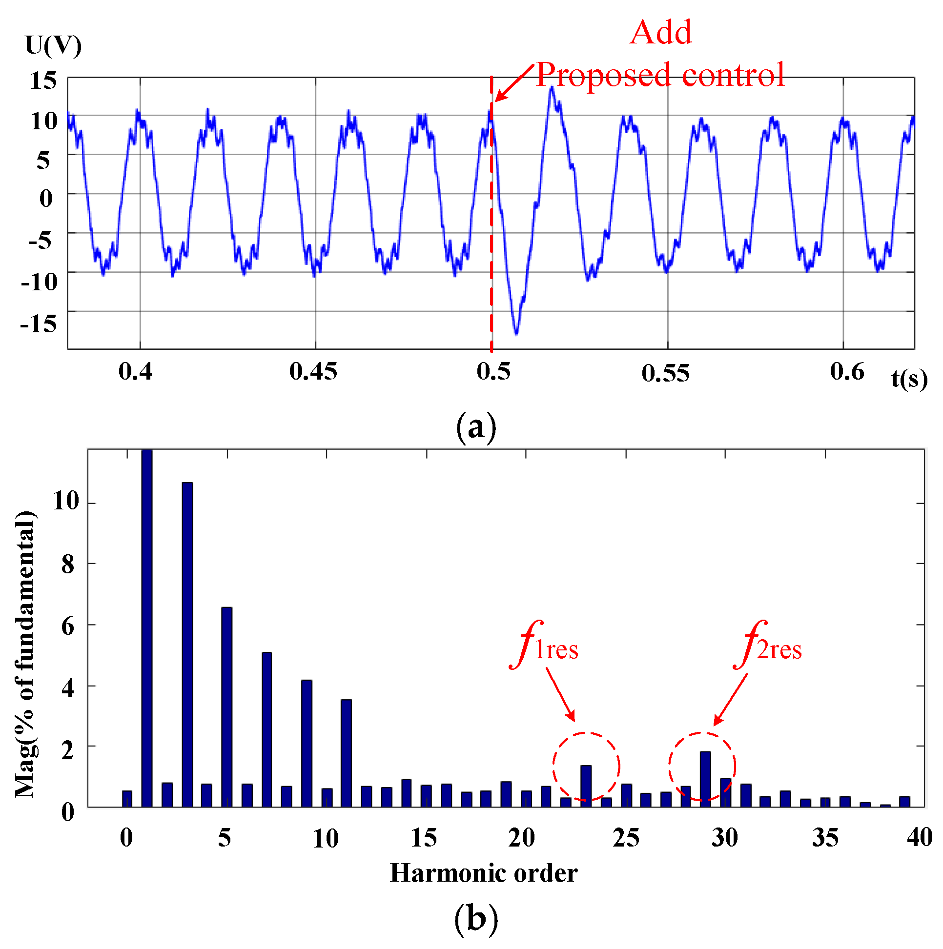
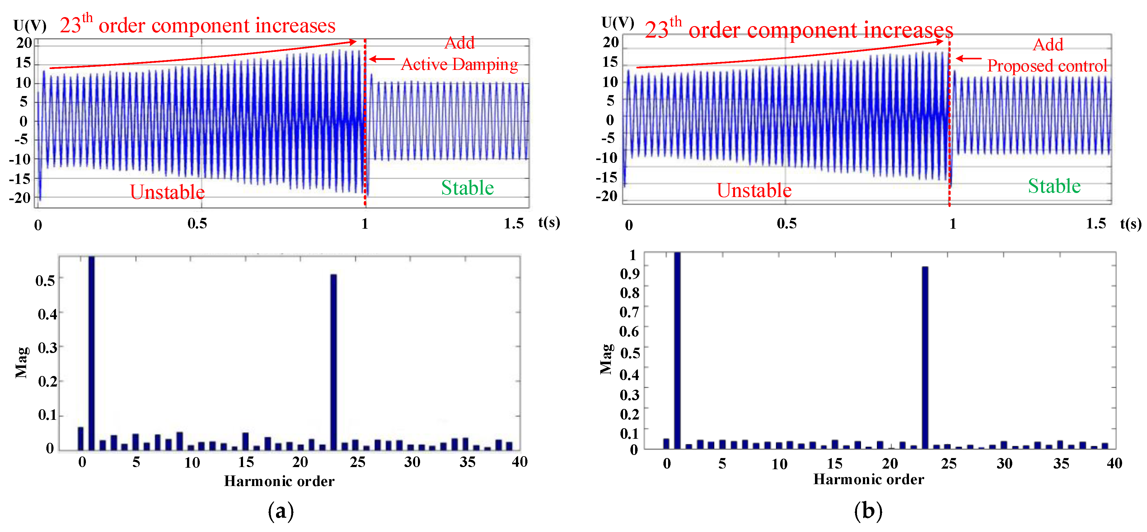
4.1.2. High-order Harmonic Results

In this simulation, the output current of HCGIs is that the RMS of fundamental current is 7.07 A and 23th order harmonic compensation current is 1 A. And the comparison between the active damping and proposed methods is shown in Figure 23.

As shown in Figure 23, the 23th order harmonic of the output current is continuously amplified which means the system is unstable before t = 1 s. In Figure 23a, the active damping method is added after t = 1 s, the system becomes stable, but the 23th order harmonic current is not soundly compensated. In Figure 23b, the proposed control method is added after t = 1 s, the system becomes stable and the compensation of the 23th order harmonic current is greatly improved. Thereby, the bandwidth issue can be solved by the proposed bandwidth control method.

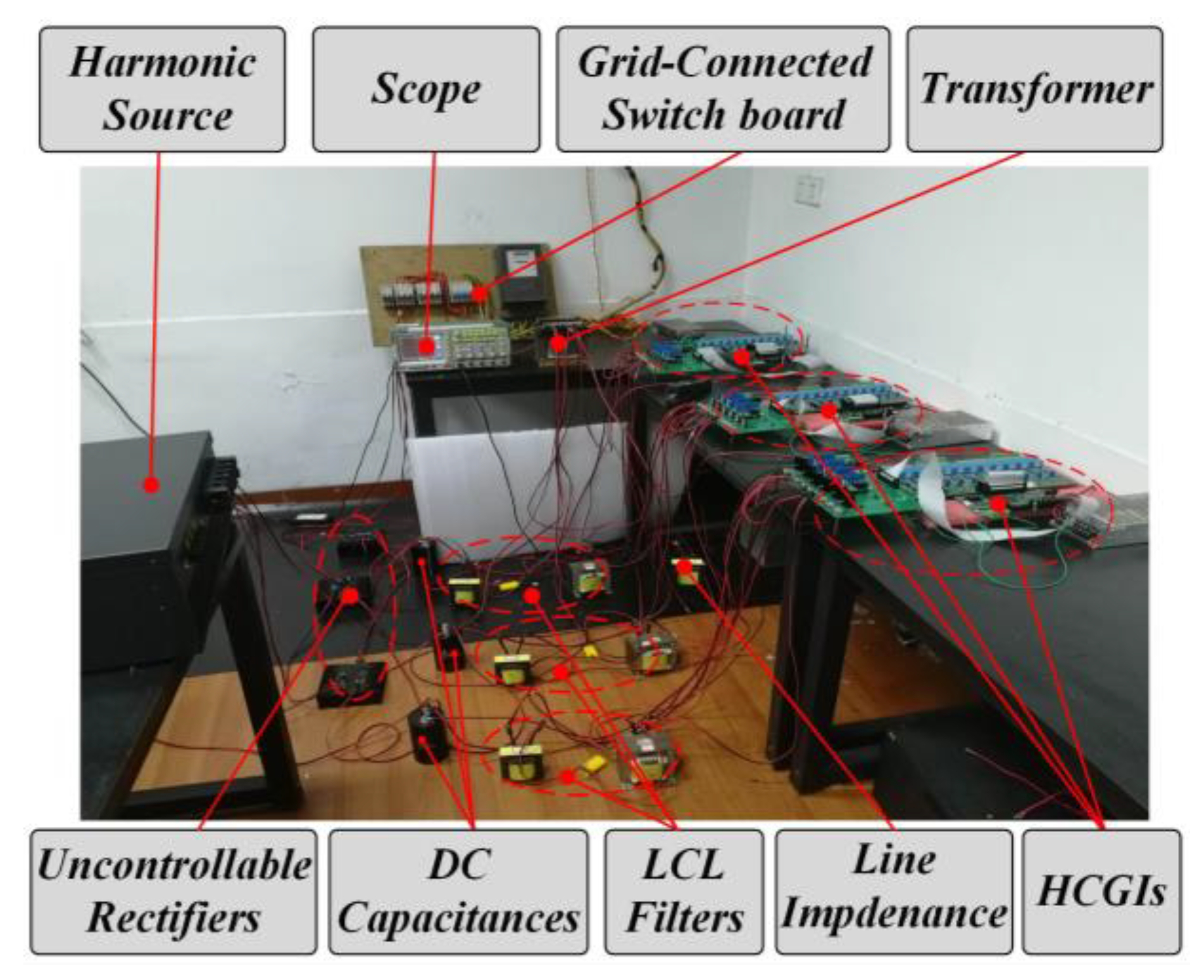
4.2. Experimental Validation

In order to further verify the proposed approach, the experimental test is conducted. As shown in Figure 24, the experimental rig is set up according to the system structure in Figure 1.

In Figure 24, the control system adopts a DSP+CPLD structure, a harmonic source is used as harmonic load, and the harmonics is mainly composed of 3rd, 5th, 7th, 9th and 11th order, the THD analysis of harmonic current is shown in Figure 25. And the electric parameters of HCGIs system and the key chips of the controller are listed in

Table 7. The electric parameters of HCGIs system and the chips used in the controller.

Symbol	Value	Symbol	Value	Chip Name	Corporation	Chip Model
L1/mH	2.8	Ug/V	110	DSP	TI	TMS320F28335
Cf/μF	10	Lg/mH	1.2	CPLD	XILINX	XC9572XL
L2/mH	1.8	fs/kHz	20	ADC	ANALOG DEVICES	AD7580

.

To illustrate the harmonic compensation at low frequency and high frequency, Figure 26 and Figure 27 show the grid current and output current of a HCGI without and with the proposed bandwidth control method, respectively. Meanwhile, the HCGIs with 23th order harmonic current and its THD analysis are shown in Figure 28.

The grid current and output current of one HCGI without bandwidth control are presented in Figure 26a and Figure 27a. When HCGIs work with the bandwidth control method, the grid current and HCGI output current are shown in Figure 26b and Figure 27b. Their THD are shown in Figure 26c,d and Figure 27c,d. The THD of HCGI output current and grid current are not affected and the frequencies of resonance points shift right.

As shown in Figure 28, without the proposed control, the HCGIs work in unstable state; after activating the bandwidth control method, the system becomes stable. From the THD analysis shown in Figure 28b, the HCGIs effectively compensate the 23th order harmonic current with the proposed method. Therefore, the experimental results of HCGIs prove the rationality and validity of the proposed bandwidth control method.

5. Conclusions

In this paper, the issue that the new resonance point of HCGIs system affects the control bandwidth has been studied. A bandwidth control method based on virtual impedance has been proposed. By shifting frequency of the resonance point to the right side, the influence of virtual resistance on high-frequency harmonics compensation is eliminated. As for the realization of capacitor voltage differential link, the high-pass filter has been used to replace the differential link equivalently in realization according to reference [32]. Some conclusions can be drawn as follows:

(1)

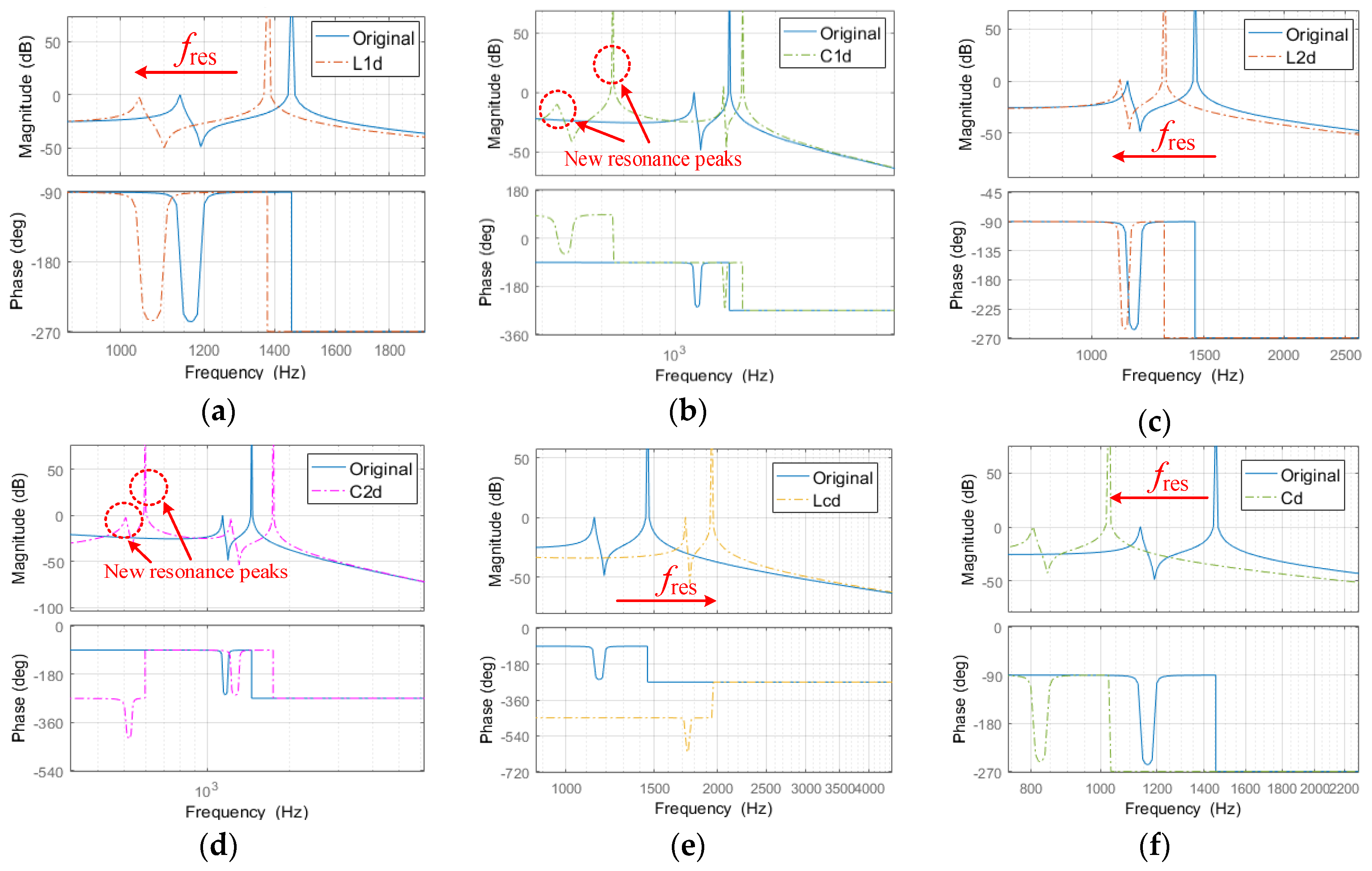
The new resonance point in multi-parallel HCGIs systems decreases the control bandwidth, thus the maximum compensation harmonic frequency of HCGIs would be limited.

(2)

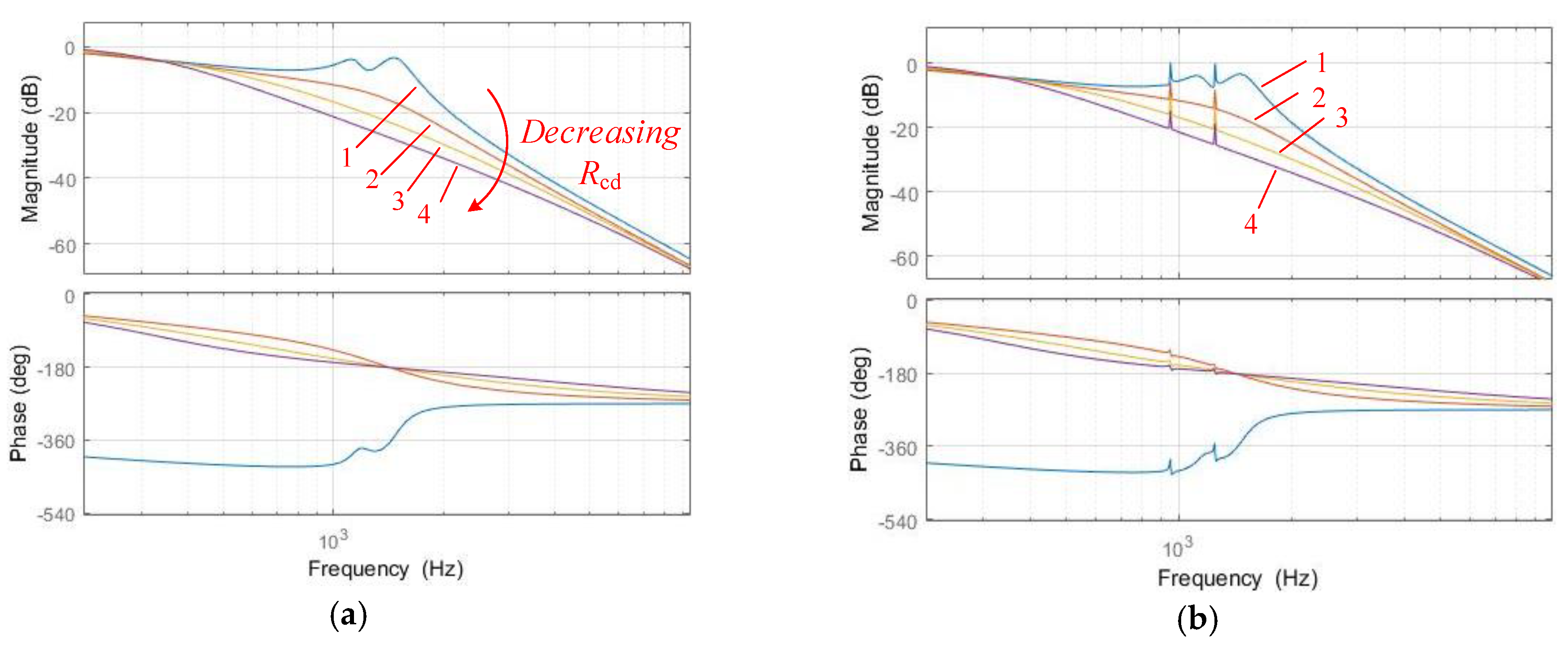
The active damping by virtual resistance to suppress resonances peak will influence the high-frequency harmonic current compensation, and the influence becomes large when the harmonic frequency approaches the LCL resonance frequency.

(3)

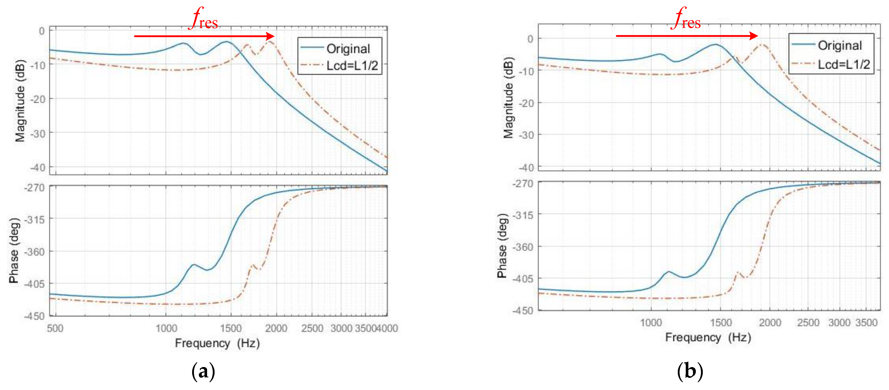
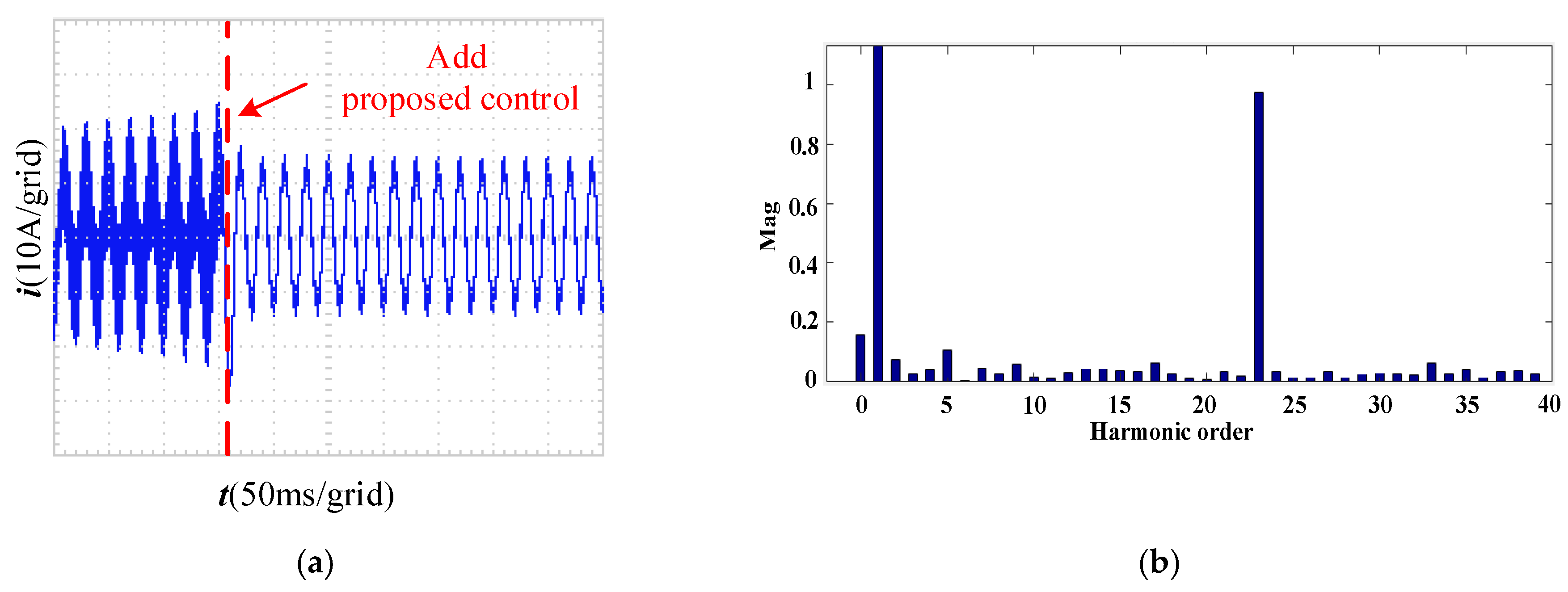
The proposed bandwidth control method can effectively shift resonance frequencies right, and thus it solves the bandwidth reduction issue in multi-parallel HCGIs system.

(4)

The bandwidth control method proposed in this paper can also solve other bandwidth issues limited by resonant frequencies for grid-connected inverters.

Finally, it is worthy pointing out that as the virtual inductance and the virtual resistance need to be considered together in the proposed method, the implementation complexity is increased compared with the active damping method.

References

1. Sun, Y.; Hou, X.; Yang, J.; Han, H.; Su, M.; Guerrero, J.M. New perspectives on droop control in AC microgrid. IEEE Trans. Ind. Electron. 2017, 64, 5741–5745. [Google Scholar] [CrossRef]
2. Zhang, N.; Tang, H.; Yao, C. A Systematic Method for Designing a PR Controller and Active Damping of the LCL Filter for Single-Phase Grid-Connected PV Inverters. Energies 2014, 7, 3934–3954. [Google Scholar] [CrossRef] [Green Version]
3. Song, D.R.; Fan, X.; Yang, J.; Liu, A.; Chen, S.; Joo, Y. Power extraction efficiency optimization of horizontal-axis wind turbines through optimizing control parameters of yaw control systems using an intelligent method. Appl. Energy 2018, 224, 267–279. [Google Scholar] [CrossRef]
4. Liu, Z.; Su, M.; Sun, Y. Optimal criterion and global/sub-optimal control schemes of decentralized economical dispatch for AC microgrid. Int. J. Electrical Power Energy Syst. 2019, 104, 38–42. [Google Scholar] [CrossRef]
5. Fadia, S.; Hani, V.; Youssef, K.H. Experimental Design of Fixed Switching Frequency Model Predictive Control for Sensor-Less Five-Level Packed U-Cell Inverter. IEEE Trans. Ind. Electron. 2018, 66, 3427–3434. [Google Scholar]
6. Song, D.; Yang, J.; Fan, X.; Liu, Y.; Liu, A.; Chen, G.; Joo, Y.H. Maximum power extraction for wind turbines through a novel yaw control solution using predicted wind directions. Energy Convers. Manag. 2018, 157, 589–599. [Google Scholar] [CrossRef]
7. Song, D.; Li, Q.; Cai, Z. Model predictive control using multi-step prediction model for electrical yaw system of horizontal-axis wind turbines. IEEE Trans. Sustain. Energy 2018. accepted. [Google Scholar] [CrossRef]
8. Vahedi, H.; Labbe, P.A.; Al-Haddad, K. Sensor-Less Five-Level Packed U-Cell Inverter Operating in Stand-Alone and Grid-Connected Modes. IEEE Trans. Ind. Inform. 2016, 12, 361–370. [Google Scholar] [CrossRef]
9. Song, D.; Yang, J.; Cai, Z.L.; Dong, M.; Joo, Y.H. Model predictive control with finite control set for variable-speed wind turbines. Energy 2017, 126, 564–572. [Google Scholar] [CrossRef]
10. Khan, S.; Zhang, X.; Saad, M. Comparative Analysis of 18-Pulse Auto transformer Rectifier Unit Topologies with Intrinsic Harmonic Current Cancellation. Energies 2018, 11, 1347. [Google Scholar] [CrossRef]
11. Zhou, N.C.; Lou, X.X.; Yu, D. Harmonic Injection-Based Power Fluctuation Control of Three-Phase PV Systems under Unbalanced Grid Voltage Conditions. Energies 2015, 8, 1390–1405. [Google Scholar] [CrossRef] [Green Version]
12. Hossain, J.; Rafi, F.; Town, G. A Multifunctional Three-Phase Four-Leg PV-SVSI with Dynamic Capacity Distribution Method. IEEE Trans. Ind. Inform. 2018, 99, 2507–2520. [Google Scholar] [CrossRef]
13. Ye, T.; Dai, N.Y.; Lam, C.S. Analysis, Design, and Implementation of a Quasi-Proportional-Resonant Controller for a Multifunctional Capacitive-Coupling Grid-Connected Inverter. IEEE Trans. Ind. Appl. 2016, 52, 4269–4280. [Google Scholar] [CrossRef]
14. Morales-Paredes, H.K.; Bonaldo, J.P.; Pomilio, J.A. Centralized Control Center Implementation for Synergistic Operation of Distributed Multifunctional Single-Phase Grid-Tie Inverters in a Microgrid. IEEE Trans. Ind. Electron. 2018, 65, 8018–8029. [Google Scholar] [CrossRef]
15. Zheng, Z.; Zhao, R.; Yang, H. A Multi-Functional Grid-Connected Inverter and Its Application to Customized Power Quality of Microgrid. Power Syst. Technol. 2012, 36, 58–67. [Google Scholar]
16. Li, X.Y.; Li, Y.L.; Zhang, W.Y. A Power Quality Control Strategy Based on Multi-Functional Grid-Connected Inverter. Power Syst. Technol. 2015, 39, 556–562. [Google Scholar]
17. Zeng, Z.; Li, H.; Tang, S. Multi-objective control of multi-functional grid-connected inverter for renewable energy integration and power quality service. IET Power Electron. 2016, 9, 761–770. [Google Scholar] [CrossRef]
18. Tang, S.; Zheng, Z.; Chong, C. Wireless Coordination Control of Multi-functional Grid-tied Inverters in Microgrid. Autom. Electr. Power Syst. 2015, 39, 200–207. [Google Scholar]
19. Agorreta, J.L.; Borrega, M.; López, J. Modeling and Control of N-Paralleled Grid-Connected Inverters with LCL Filter Coupled Due to Grid Impedance in PV Plants. IEEE Trans. Power Electron. 2011, 26, 770–785. [Google Scholar] [CrossRef]
20. He, J.; Li, Y.W.; Bosnjak, D. Investigation and Active Damping of Multiple Resonances in a Parallel-Inverter-Based Microgrid. IEEE Trans. Power Electron. 2013, 28, 234–246. [Google Scholar] [CrossRef]
21. Zeng, Z.; Zhao, R.X.; Lv, Z.P. Impedance Reshaping of Grid-tied Inverters to Damp the Series and Parallel Harmonic Resonances of Photovoltaic Systems. Proc. Csee 2014, 34, 4547–4558. [Google Scholar]
22. Kuang, H.; An, L.; Chen, Z. Coupling Resonances Mechanism of Grid-Connected Multi-Parallel Inverters and Its Active Damping Parameter Optimal Method. Power Syst. Technol. 2016, 40, 1180–1189. [Google Scholar]
23. Lu, X.N.; Sun, K.; Huang, L.P. Active Damping Method Based on Bi-Quad Filter for Microgrid Applications. Trans. China Electrotech. Soc. 2013, 28, 261–268. [Google Scholar]
24. Zhang, S.; Jiang, S.; Lu, X. Resonance issues and damping techniques for grid-connected inverters with long transmission cable. IEEE Trans. Power Electron. 2013, 29, 110–120. [Google Scholar] [CrossRef]
25. Hu, W.; Sun, J.; Ma, Q. Modeling and resonant characteristics analysis of multiple paralleled grid-connected inverters with LCL filter. In Proceedings of the 2014 IEEE Energy Conversion Congress and Exposition, Pittsburgh, PA, USA, 14–18 September 2014; pp. 3371–3377. [Google Scholar]
26. Turner, R.; Walton, S.; Duke, R. Stability and Bandwidth Implications of Digitally Controlled Grid-Connected Parallel Inverters. IEEE Trans. Ind. Electron. 2010, 11, 3685–3694. [Google Scholar] [CrossRef]
27. Parker, S.G.; Mcgrath, B.P.; Holmes, D.G. Regions of active damping control for LCL filters. In Proceedings of the 2012 IEEE Energy Conversion Congress and Exposition, Raleigh, NC, USA, 15–20 September 2012; pp. 53–60. [Google Scholar]
28. Wang, J.; Yan, J.D.; Jiang, L. Delay-Dependent Stability of Single-Loop Controlled Grid-Connected Inverters with LCL Filters. IEEE Trans. Power Electron. 2015, 31, 743–757. [Google Scholar] [CrossRef]
29. Wang, X.; Loh, P.C.; Blaabjerg, F. Stability Analysis and Controller Synthesis for Single-Loop Voltage-Controlled VSIs. IEEE Trans. Power Electron. 2017, 32, 7394–7404. [Google Scholar] [CrossRef] [Green Version]
30. Xu, J.; Xie, S.; Zhang, B. Robust Grid Current Control with Impedance-Phase Shaping for LCL-Filtered Inverters in Weak and Distorted Grid. IEEE Trans. Power Electron. 2018, 99, 10240–10250. [Google Scholar] [CrossRef]
31. He, J.; Li, Y.W.; Blaabjerg, F. An Enhanced Islanding Microgrid Reactive Power, Imbalance Power, and Harmonic Power Sharing Scheme. IEEE Trans. Power Electron. 2015, 30, 3389–3401. [Google Scholar] [CrossRef]
32. Ruan, X.; Wang, X.; Pan, D.; Yang, D. Control Techniques for LCL-Type Grid-Connected Inverters, 1st ed.; Science Press Beijing: Beijing, China, 2018; pp. 79–94. ISBN 978-7-03-043810-2. [Google Scholar]
33. Yang, Y.; Zhou, K.; Blaabjerg, F. Current harmonics from single-phase grid-connected inverters—Examination and suppression. IEEE J. Emerg. Sel. Top. Power Electron. 2016, 4, 221–233. [Google Scholar] [CrossRef]
34. Malinowski, M.; Bernet, S. A Simple Voltage Sensorless Active Damping Scheme for Three-Phase PWM Converters with an Filter. IEEE Trans. Ind. Electron. 2008, 55, 1876–1880. [Google Scholar] [CrossRef]
Figure 1. Configuration of a multi-parallel HCGIs system.
Energies 12 00571 g001
Figure 2. Implified model of LCL filter network for Go_m.
Energies 12 00571 g002
Figure 3. Bode diagram of Go_m.
Energies 12 00571 g003
Figure 4. The control diagram of output current loop.
Energies 12 00571 g004
Figure 5. The Norton equivalent circuit of multi-parallel HCGIs system.
Energies 12 00571 g005
Figure 6. The Bode diagram of ΦO_m with difference n.
Energies 12 00571 g006
Figure 7. Zero pole diagram of single HCGI and multi-parallel HCGIs system.
Energies 12 00571 g007
Figure 8. The LCL filter equivalent circuit and control block diagram: (a) The LCL filter equivalent circuit; (b) The control block diagram.
Energies 12 00571 g008
Figure 9. Bode diagram of 3-parallel HCGIs with different Rcd: (a) Without high-frequency harmonics compensation; (b) With high-frequency harmonics compensation.
Energies 12 00571 g009
Figure 10. Virtual impedance equivalent circuits of actual LCL filter. (a) L1d; (b) C1d; (c) L2d; (d) C2d; (e) LCd; (f) Cd.
Energies 12 00571 g010
Figure 11. Virtual impedance bode diagrams of Go_m: (a) L1d; (b) C1d; (c) L2d; (d) C2d; (e) LCd; (f) Cd.
Energies 12 00571 g011
Figure 12. Equivalent control diagram of output current loop with virtual inductance.
Energies 12 00571 g012
Figure 13. Bode diagram of multi-parallel HCGIs with. L c d = L 1 / 2 . (a) n = 3; (b) n = 5.
Energies 12 00571 g013
Figure 14. Generalized equivalent circuit for the bandwidth control method.
Energies 12 00571 g014
Figure 15. Equivalent control diagram. (a) Capacitor current feedback; (b) Capacitor voltage feedback.
Energies 12 00571 g015aEnergies 12 00571 g015b
Figure 16. Bode diagram of multi-parallel HCGIs with difference λ L .
Energies 12 00571 g016
Figure 17. Bode diagram of 3-parallel HCGIs under two methods. (a) Fundamental; (b) With high-frequency harmonics.
Energies 12 00571 g017aEnergies 12 00571 g017b
Figure 18. Power output of the three HCGIs.
Energies 12 00571 g018
Figure 19. Grid current and THD analysis. (a) Grid current; (b) THD analysis (Fundamental component = 29.74 A, THD = 13.91%).
Energies 12 00571 g019
Figure 20. Grid current and its THD analysis. (a) Grid current; (b) before t =0.5 s (fundamental component = 29.59 A, THD = 2.15%); (c) before t = 0.5 s (fundamental component = 29.64 A, THD = 2.01%).
Energies 12 00571 g020aEnergies 12 00571 g020b
Figure 21. Output current of HCGI and its THD analysis. (a) Output current of HCGI; (b) THD before t = 0.5 s (fundamental component = 9.851 A, THD = 16.56%); (c) THD after t = 0.5 s (fundamental component = 9.762 A, THD = 15.97%).
Energies 12 00571 g021aEnergies 12 00571 g021b
Figure 22. Output current of HCGI, grid current and them THD analysis. (a) Output current of HCGI and its THD after t = 0.5 s (fundamental component = 9.5151 A, THD = 31.43%); (b) Grid current and its THD after t = 0.5 s (fundamental component = 29.462 A, THD = 2.87%).
Energies 12 00571 g022
Figure 23. Output current and its THD analysis of HCGI. (a) Output current of HCGI and its THD analysis after t = 1 s with active damping (fundamental component = 9.73 A, 23th current component = 0.52 A, THD = 5.73%); (b) Output current of HCGI and its THD analysis after t = 1 s with proposed control (fundamental component = 9.686 A, 23th current component = 0.912 A, THD = 9.58%).
Energies 12 00571 g023
Figure 24. The experimental platform.
Energies 12 00571 g024
Figure 25. The THD analysis of harmonic load current.
Energies 12 00571 g025
Figure 26. Grid current, HCGI output current and their THD analysis without Gd. (a) Output current; (b) Grid current; (c) Output-current THD analysis (fundamental component = 29.45 A, THD = 3.43%); (d) Grid-current THD analysis (fundamental component = 9.686 A, THD = 15.23%).
Energies 12 00571 g026
Figure 27. Grid current, HCGI output current and their THD analysis with Gd. (a) Output current; (b) Grid current; (c) Output-current THD analysis (fundamental component = 29.249 A, THD = 2.57%); (d) Grid-current THD analysis (fundamental component = 9.814 A, THD = 14.17%).
Energies 12 00571 g027
Figure 28. The HCGI output current with 23th order harmonic current. (a) Output current; (b) THD analysis (fundamental component = 9.734 A, 23th current component = 0.925 A, THD = 12.07%).
Energies 12 00571 g028