Reliability Enhancement in Power Networks under Uncertainty from Distributed Energy Resources †


Abstract
1. Introduction
2. MV and LV Distribution Network Design
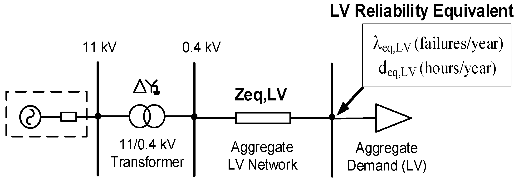
2.1. Electrical and Reliability Network Equivalents
- (1)
- Calculate equivalent impedance at every network load location. This includes multiple customers at the same bus or supply point, and is expressed by Equation (1).
- (2)
- Sum all equivalent impedances calculated in Step 1 to determine the overall network impedance. This is described by Equation (2):where: Ni is the number of customers at load location i, I is the number of load locations, Zcustomer (ni) is the impedance of the customer ni at location i, Zlocation(i) is the sum of all customer impedances at location i, and Zeq, Req and Xeq are the equivalent impedance, resistance and reactance, respectively.
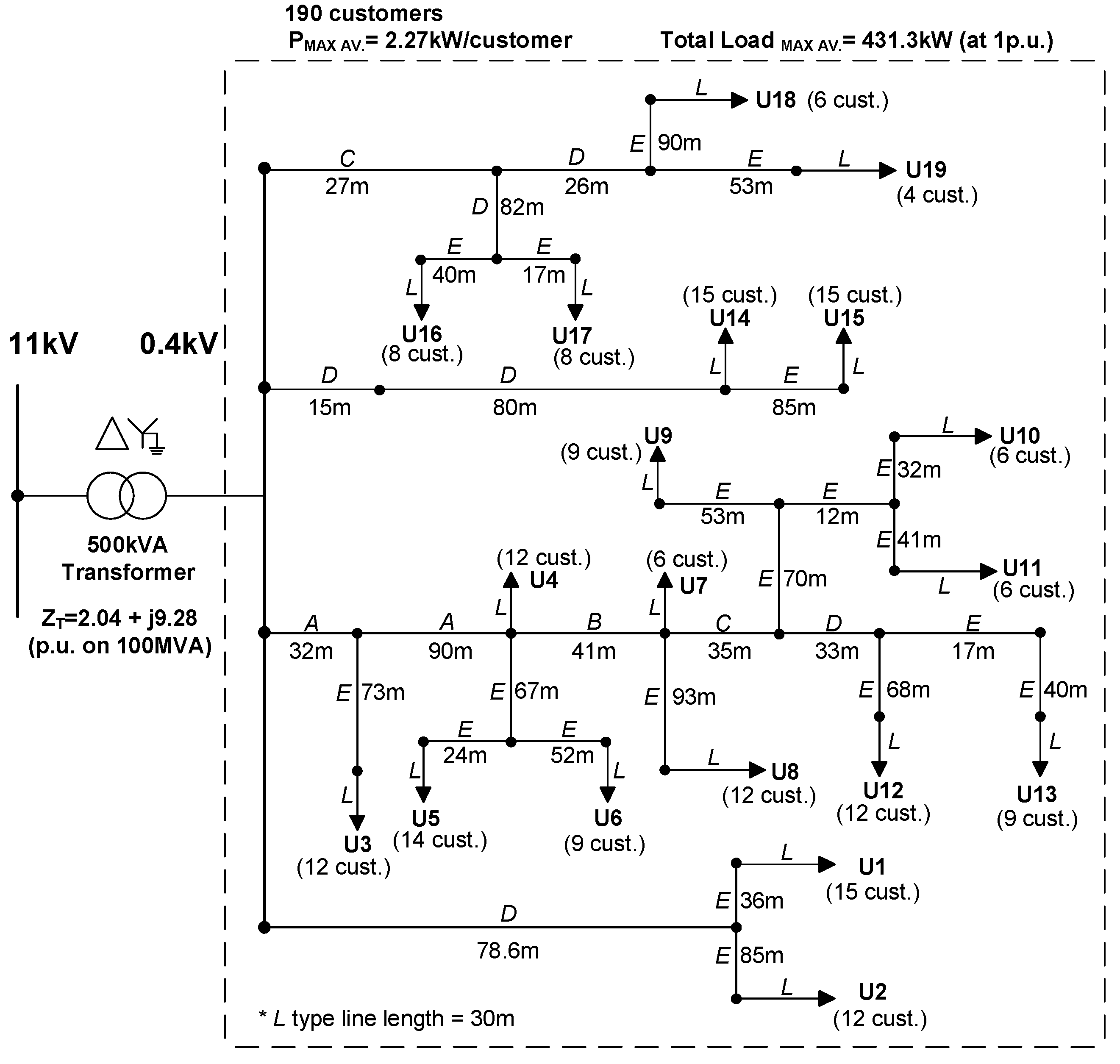
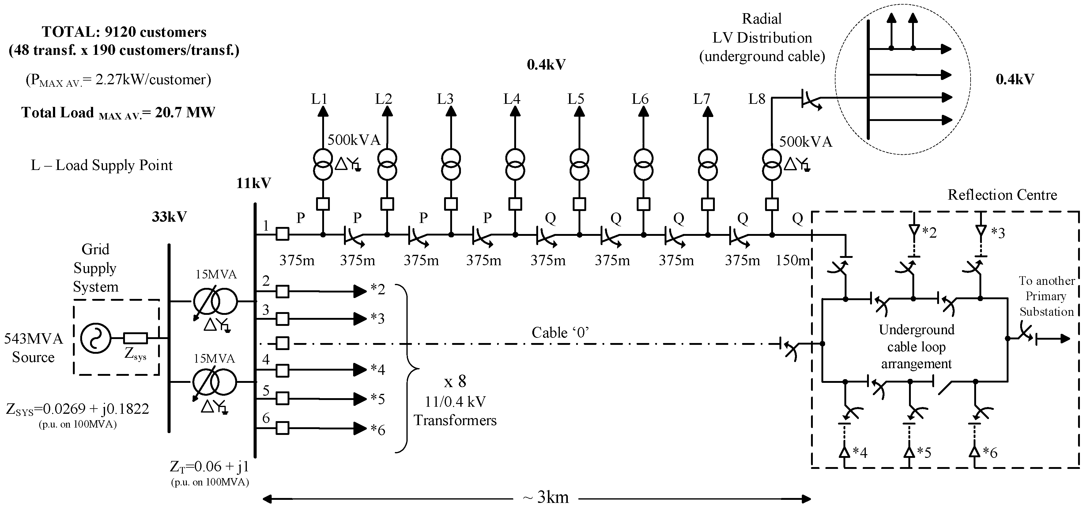
2.2. Urban MV/LV Distribution Network
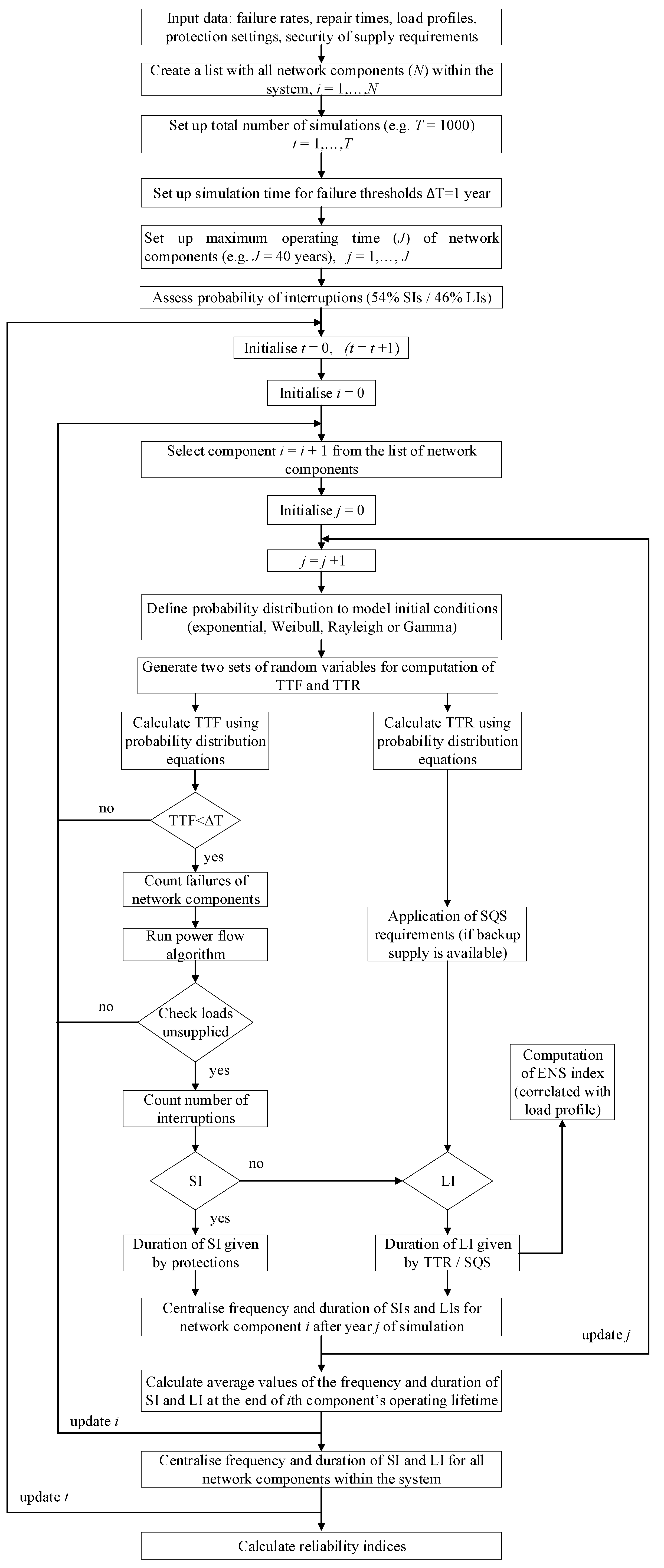
3. Reliability Assessment Methodology
4. Network Scenarios Incorporating Smart Interventions
4.1. SC-1: Base Case
4.2. SC-2: Demand-Side Response (DSR)
4.3. SC-3: Uncontrolled PV
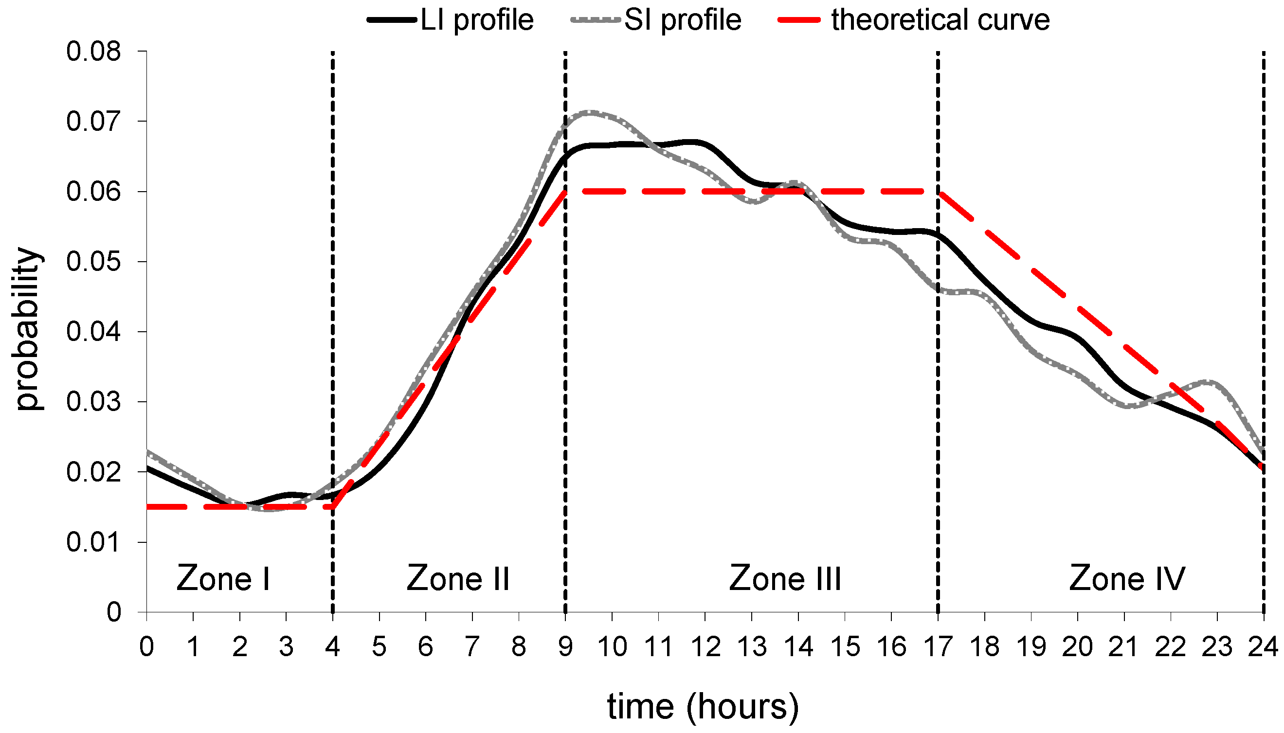
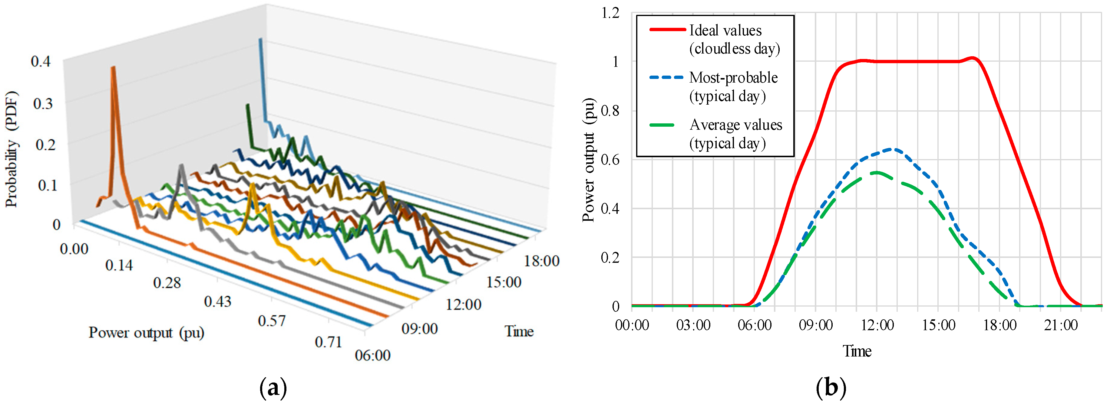
4.3.1. Temporal Variation of Solar Energy Resources
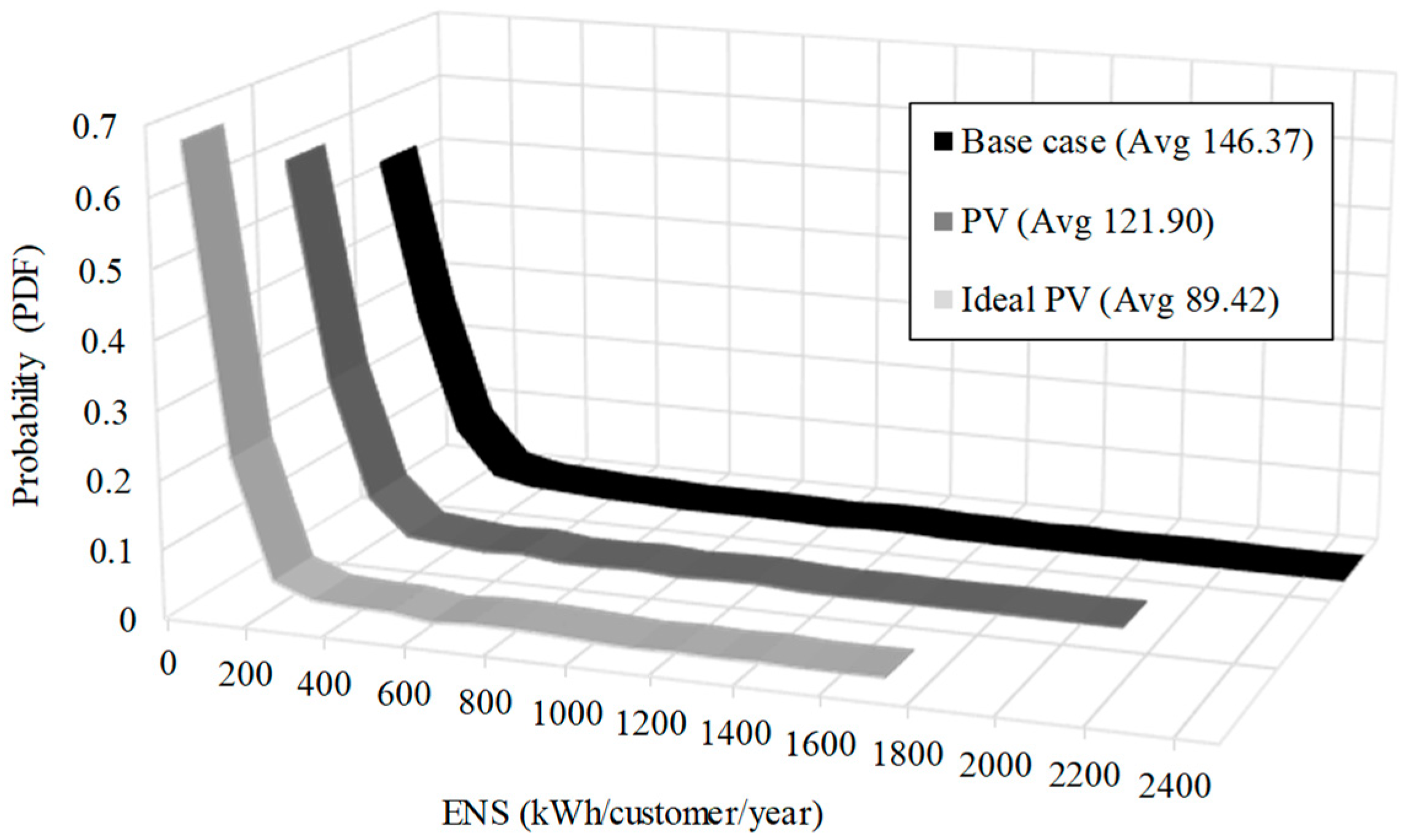
4.3.2. Impact of Clouding Effect on Reliability Performance
4.3.3. SC-4: PV+DSR
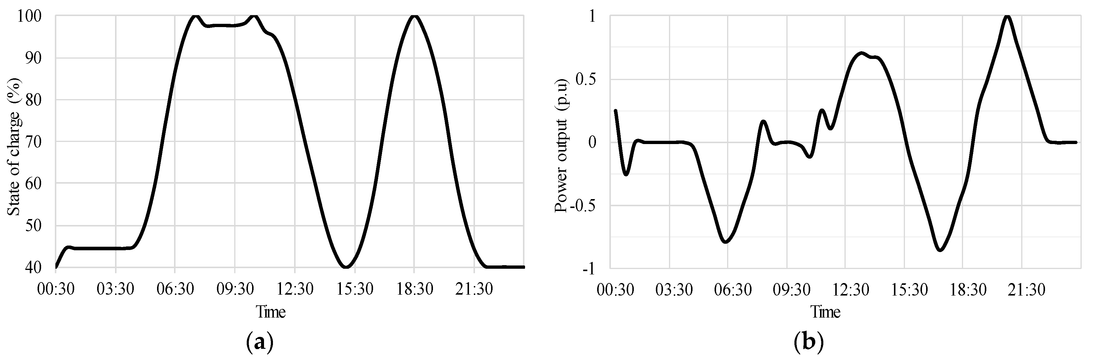
4.4. SC-5: Energy Storage (ES)
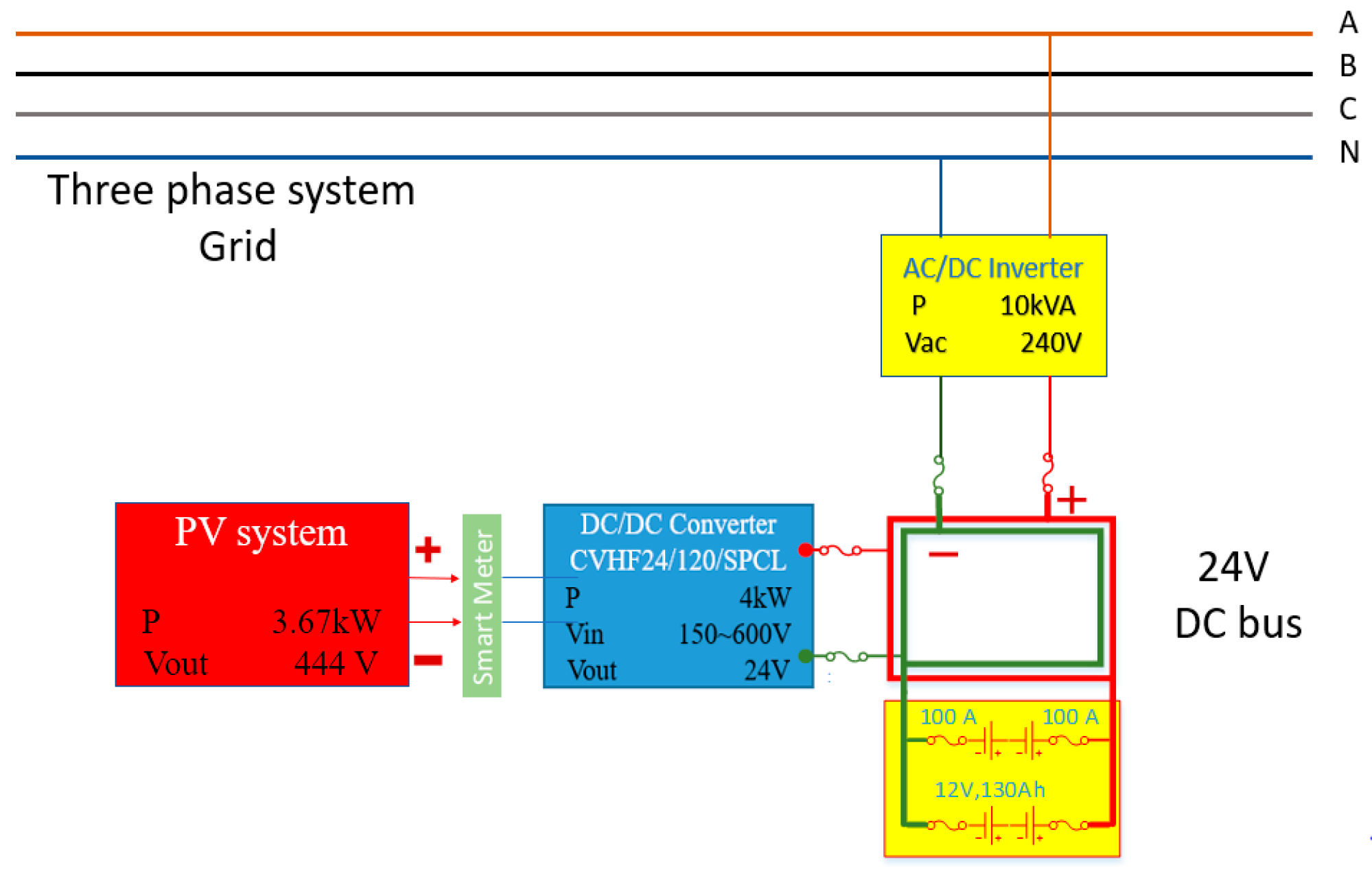
4.4.1. ES System Configuration
4.4.2. ES System Operation
4.4.3. SC-6: ES + DSR
5. Reliability Performance Assessment
5.1. Impact on Frequency of Interruptions
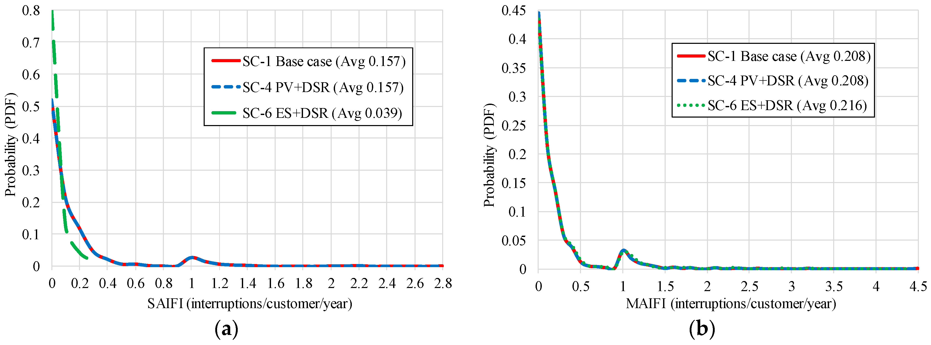
5.1.1. System-Oriented Frequency of Interruption Indices
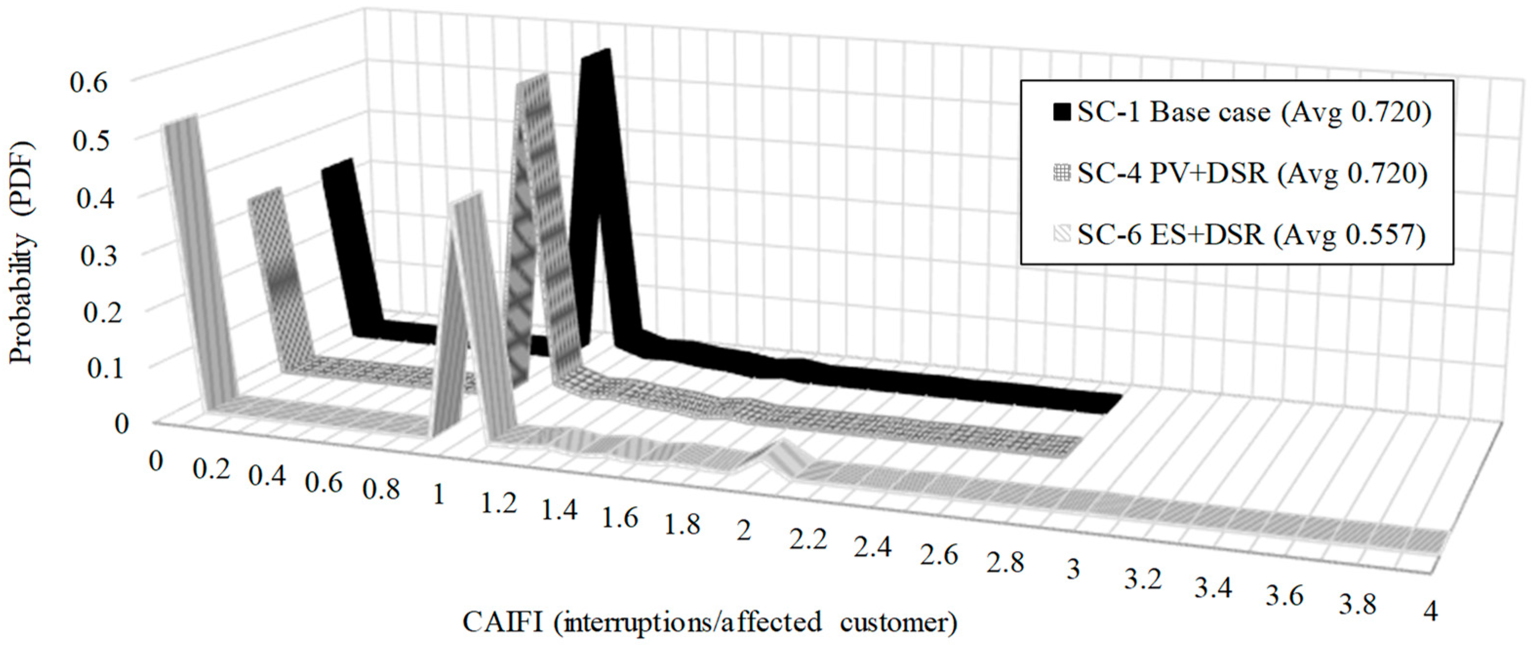
5.1.2. Customer-Oriented Frequency of Interruption Indices
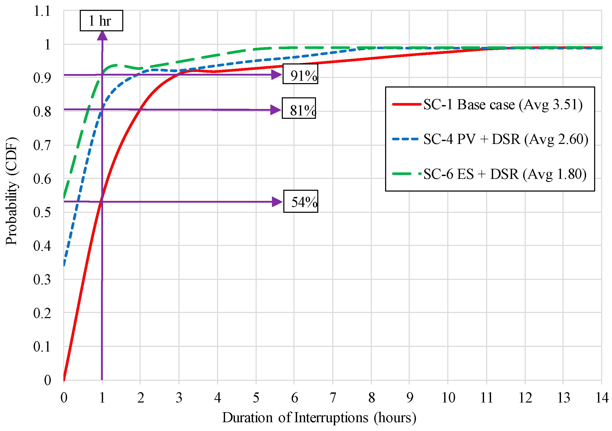
5.2. Impact on Duration of Sustained Interruptions
5.2.1. System-Oriented Duration of Interruption Indices
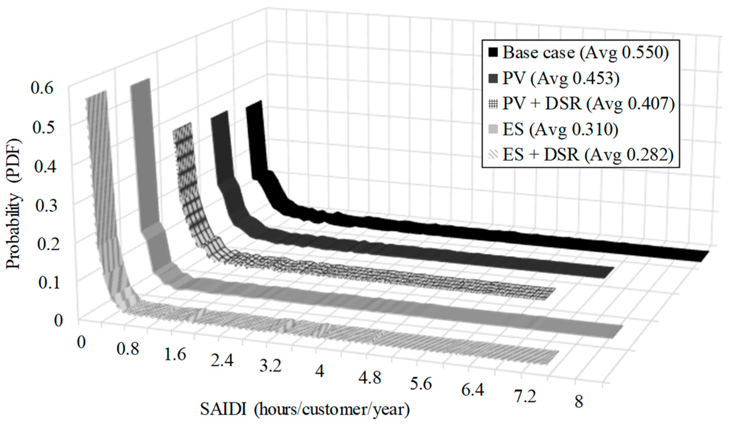
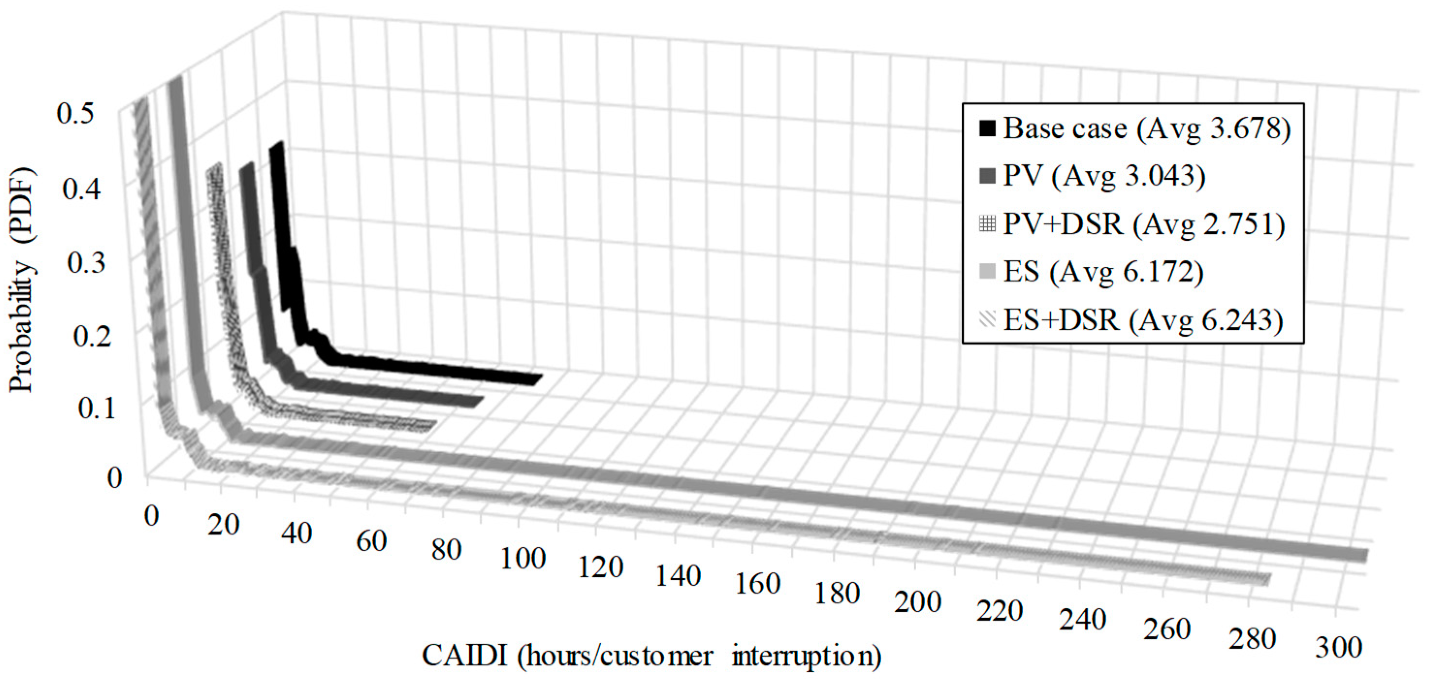
5.2.2. Customer-Oriented Duration of Interruption Indices
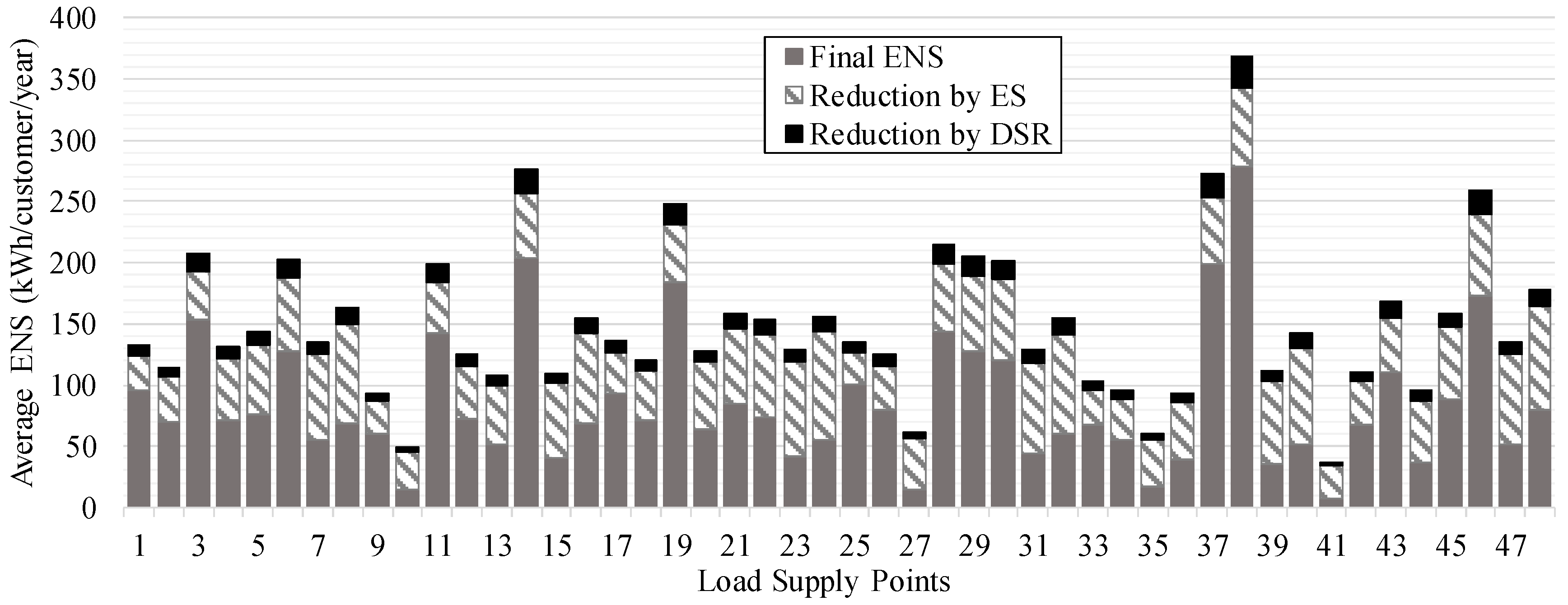
5.3. Impact on Energy Not Supplied
5.3.1. Average Energy Not Supplied
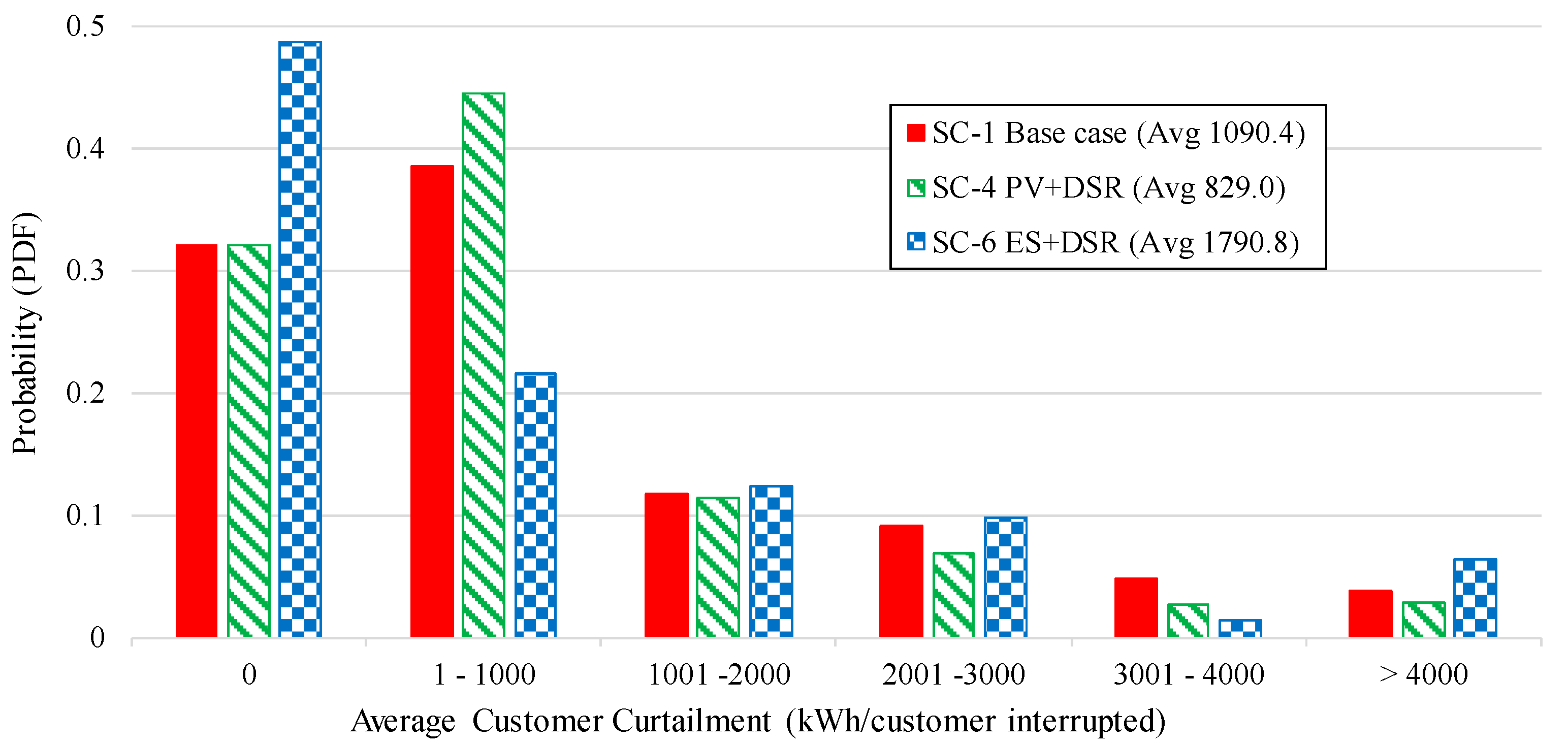
5.3.2. Average Customer Curtailment
6. Conclusions
Author Contributions
Acknowledgments
Conflicts of Interest
References
- FERC. Title XIII: Smart Grid. In Energy Independence and Security Act of 2007; 110th United States Congress: Washington, DC, USA, 2007. [Google Scholar]
- Hernando-Gil, I.; Ilie, I.S.; Collin, A.J.; Acosta, J.L.; Djokic, S.Z. Impact of DG and energy storage on distribution network reliability: A comparative analysis. In Proceedings of the 2012 IEEE International Energy Conference and Exhibition (ENERGYCON), Florence, Italy, 9–12 September 2012. [Google Scholar]
- NationalGridESO. Balancing Services. Available online: https://www.nationalgrideso.com/balancing-services (accessed on 10 October 2018).
- Ndawula, M.B.; Hernando-Gil, I.; Djokic, S. Impact of the stochastic behaviour of distributed energy resources on MV/LV network reliability. In Proceedings of the 2018 IEEE International Conference on Environment and Electrical Engineering and 2018 IEEE EEEIC/I&CPS Europe), Palermo, Italy, 12–15 June 2018; pp. 1–6. [Google Scholar]
- Wang, Y.; Lin, X.; Pedram, M. Adaptive control for energy storage systems in households with photovoltaic modules. IEEE Trans. Smart Grid 2014, 5, 992–1001. [Google Scholar] [CrossRef]
- OFGEM. The Electricity (Connection Standards of Performance) Regulations; OFGEM: London, UK, 2015.
- ENA. Engineering Recommendation p2-6, Security of Supply; Energy Networks Association (ENA); ENA: London, UK, 2005. [Google Scholar]
- IEEE Guide for Electric Power Distribution Reliability Indices; IEEE Std 1366-2003; IEEE: Washington, DC, USA, 2004; pp. 1–50.
- Ndawula, M.B.; Zhao, P.; Hernando-Gil, I. Smart application of energy management systems for distribution network reliability enhancement. In Proceedings of the 2018 IEEE International Conference on Environment and Electrical Engineering and 2018 IEEE EEEIC/I&CPS Europe, Palermo, Italy, 12–15 June 2018; pp. 1–5. [Google Scholar]
- Alam, M.J.E.; Muttaqi, K.M.; Sutanto, D. A novel approach for ramp-rate control of solar PV using energy storage to mitigate output fluctuations caused by cloud passing. IEEE Trans. Energy Convers. 2014, 29, 507–518. [Google Scholar]
- Bass, R.B.; Carr, J.; Aguilar, J.; Whitener, K. Determining the power and energy capacities of a battery energy storage system to accommodate high photovoltaic penetration on a distribution feeder. IEEE Power Energy Technol. Syst. J. 2016, 3, 119–127. [Google Scholar] [CrossRef]
- Faza, A. A probabilistic model for estimating the effects of photovoltaic sources on the power systems reliability. Reliab. Eng. Syst. Saf. 2018, 171, 67–77. [Google Scholar] [CrossRef]
- Adefarati, T.; Bansal, R.C. Reliability, economic and environmental analysis of a microgrid system in the presence of renewable energy resources. Appl. Energy 2019, 236, 1089–1114. [Google Scholar] [CrossRef]
- Sa’ed, J.; Favuzza, S.; Massaro, F.; Telaretti, E. Optimization of bess capacity under a peak load shaving strategy. In Proceedings of the 2018 IEEE International Conference on Environment and Electrical Engineering and 2018 IEEE Industrial and Commercial Power Systems Europe (EEEIC/I&CPS Europe), Palermo, Italy, 12–15 June 2018; pp. 1–4. [Google Scholar]
- Zheng, Y.; Meng, K.; Luo, F.; Qiu, J.; Zhao, J. Optimal integration of MBESSS/SBESSS in distribution systems with renewables. IET Renew. Power Gener. 2018, 12, 1172–1179. [Google Scholar] [CrossRef]
- Qiao, Z.; Yang, J. Comparison of centralised and distributed battery energy storage systems in LV distribution networks on operational optimisation and financial benefits. J. Eng. 2017, 2017, 1671–1675. [Google Scholar] [CrossRef]
- Mohamad, F.; Teh, J. Impacts of energy storage system on power system reliability: A systematic review. Energies 2018, 11, 1749. [Google Scholar] [CrossRef]
- Hernando-Gil, I.; Hayes, B.; Collin, A.; Djokić, S. Distribution network equivalents for reliability analysis. Part 1: Aggregation methodology. In Proceedings of the IEEE PES ISGT Europe 2013, Lyngby, Denmark, 6–9 October 2013; pp. 1–5. [Google Scholar]
- Jasmon, G.B.; Lee, L.H.C.C. Distribution network reduction for voltage stability analysis and loadflow calculations. Int. J. Electr. Power Energy Syst. 1991, 13, 9–13. [Google Scholar] [CrossRef]
- Trichakis, P.; Taylor, P.C.; Lyons, P.F.; Hair, R. Predicting the technical impacts of high levels of small-scale embedded generators on low-voltage networks. IET Renew. Power Gener. 2008, 2, 249–262. [Google Scholar] [CrossRef]
- Billinton, R.; Allan, R.N. Reliability Evaluation of Power Systems; Springer: Boston, MA, USA, 1984. [Google Scholar]
- Billinton, R.; Sankarakrishnan, A. A comparison of monte carlo simulation techniques for composite power system reliability assessment. In Proceedings of the IEEE WESCANEX 95. Communications, Power, and Computing. Conference Proceedings, Winnipeg, MB, Canada, 15–16 May 1995; Volume 141, pp. 145–150. [Google Scholar]
- Billinton, R.; Jonnavithula, A. Application of sequential monte carlo simulation to evaluation of distributions of composite system indices. IEE Proc. Gener. Transm. Distrib. 1997, 144, 87–90. [Google Scholar] [CrossRef]
- Hernando-Gil, I.; Ilie, I.S.; Djokic, S.Z. Reliability planning of active distribution systems incorporating regulator requirements and network-reliability equivalents. IET Gener. Transm. Distrib. 2016, 10, 93–106. [Google Scholar] [CrossRef]
- Hernando Gil, I. Integrated Assessment of Quality of Supply in Future Electricity Networks; The University of Edinburgh: Edinburgh, Scotland, UK, 2014. [Google Scholar]
- Ilie, I.; Hernando-Gil, I.; Djokic, S.Z. Reliability equivalents of LV and MV distribution networks. In Proceedings of the 2012 IEEE International Energy Conference and Exhibition (ENERGYCON), Florence, Italy, 9–12 September 2012; pp. 343–348. [Google Scholar]
- Hadjsaïd, N.; Sabonnadière, J.C. Electrical Distribution Networks; Wiley: Hoboken, NJ, USA, 2013. [Google Scholar]
- Martinez-Velasco, A.J.; Guerra, G. Reliability analysis of distribution systems with photovoltaic generation using a power flow simulator and a parallel monte carlo approach. Energies 2016, 9, 537. [Google Scholar] [CrossRef]
- Hernando-Gil, I.; Ilie, I.S.; Djokic, S.Z. Reliability performance of smart grids with demand-side management and distributed generation/storage technologies. In Proceedings of the 2012 3rd IEEE PES Innovative Smart Grid Technologies Europe (ISGT Europe), Berlin, Germany, 14–17 October 2012; pp. 1–8. [Google Scholar]
- Hernando-Gil, I.; Hayes, B.; Collin, A.; Djokić, S. Distribution network equivalents for reliability analysis. Part 2: Storage and demand-side resources. In Proceedings of the IEEE PES ISGT Europe 2013, Lyngby, Denmark, 6–9 October 2013; pp. 1–5. [Google Scholar]
- High Penetration of PV Systems into the Distribution Grid; U.S. Department of Energy: Washing, DC, USA, 2009.
- Mather, B.; Neal, R. Integrating high penetrations of PV into southern california: Year 2 project update. In Proceedings of the 2012 38th IEEE Photovoltaic Specialists Conference, Austin, TX, USA, 3–8 June 2012; pp. 000737–000741. [Google Scholar]
- Smith, J.W.; Dugan, R.; Sunderman, W. Distribution modeling and analysis of high penetration PV. In Proceedings of the 2011 IEEE Power and Energy Society General Meeting, Detroit, MI, USA, 24–29 July 2011; pp. 1–7. [Google Scholar]
- Smith, J.W.; Dugan, R.; Rylander, M.; Key, T. Advanced distribution planning tools for high penetration PV deployment. In Proceedings of the 2012 IEEE Power and Energy Society General Meeting, San Diego, CA, USA, 22–26 July 2012; pp. 1–7. [Google Scholar]
- Chang, G.W.; Chen, Y.H.; Hsu, L.Y.; Chen, Y.Y.; Chang, Y.R.; Lee, Y.D. Study of impact on high PV-penetrated feeder voltage due to moving cloud shadows. In Proceedings of the 2016 International Symposium on Computer, Consumer and Control (IS3C), Xi’an, China, 4–6 July 2016; pp. 1067–1070. [Google Scholar]
- Graabak, I.; Korpås, M. Variability characteristics of european wind and solar power resources—A review. Energies 2016, 9, 449. [Google Scholar] [CrossRef]
- Zhang, D.; Guo, J.; Li, J. Coordinated control strategy of hybrid energy storage to improve accommodating ability of PV. J. Eng. 2017, 2017, 1555–1559. [Google Scholar] [CrossRef]
- ENA. Engineering Recommendation g83 Energy Networks Association (ENA); ENA: London, UK, 2018. [Google Scholar]
- Zhao, P.; Hernando-Gil, I.; Wu, H. Optimal energy operation and scalability assessment of microgrids for residential services. In Proceedings of the 2018 IEEE International Conference on Environment and Electrical Engineering and 2018 IEEE Industrial and Commercial Power Systems Europe (EEEIC), Palermo, Italy, 12–15 June 2018; pp. 1–6. [Google Scholar]
- Lili, C.; Longhua, M.; Zhong, L. Analysis of the operating characteristics of a PV-diesel-BESS microgrid system. Power Syst. Prot. Control 2015, 43, 86–91. [Google Scholar]
- Wang, F.; Zhou, L.; Ren, H.; Liu, X.; Talari, S.; Shafie-khah, M.; Catalão, J.P.S. Multi-objective optimization model of source–load–storage synergetic dispatch for a building energy management system based on tou price demand response. IEEE Trans. Ind. Appl. 2018, 54, 1017–1028. [Google Scholar] [CrossRef]
- Zhao, P.; Wu, H.; Hernando-Gil, I. Optimal home energy management under hybrid PV-storage uncertainty: A distributionally robust chance constrained approach. IET Renew. Power Gener. 2018. Submitted. [Google Scholar]
- Zhao, C.; Dong, S.; Gu, C.; Li, F.; Song, Y.; Padhy, N.P. New problem formulation for optimal demand side response in hybrid ac/dc systems. IEEE Trans. Smart Grid 2018, 9, 3154–3165. [Google Scholar] [CrossRef]
- TrinaSolar. TSM_PD14 Datasheet B. Product Datasheet; TrinaSolar: San Jose, CA, USA, 2017. [Google Scholar]
- McDermott, T.E.; Dugan, R.C. Distributed generation impact on reliability and power quality indices. In Proceedings of the 2002 Rural Electric Power Conference, Papers Presented at the 46th Annual Conference (Cat. No. 02CH37360), Colorado Springs, CO, USA, 5–7 May 2002. [Google Scholar]


| ID | Network Scenario | Description |
|---|---|---|
| SC-1 | Base case | Inclusion of backup capability and SQS regulations |
| SC-2 | DSR | Demand-side response for reliability improvement |
| SC-3 | PV | Uncontrolled MG using the most probable PV power output |
| SC-4 | PV + DSR | Combination of PV and DSR |
| SC-5 | ES | EMS-Controlled MG supplying energy per customer per fault |
| SC-6 | ES + DSR | Application of ES after DSR |
| Index | Base case | PV | * | Ideal PV | * | Clouding Effect |
|---|---|---|---|---|---|---|
| ENS (kWh/cust./y) | 146.37 | 121.90 | 16.7% | 89.42 | 38.9% | 22.2% |
| ACCI (kWh/cust. int.) | 1090.41 | 909.75 | 16.6% | 664.17 | 39.1% | 22.5% |
| SAIDI (hours/cust./y) | 0.550 | 0.453 | 17.7% | 0.332 | 39.6% | 22.0% |
| CAIDI (hours/cust. int.) | 3.678 | 3.043 | 17.3% | 2.228 | 39.4% | 22.2% |
| Scenario | MAIFI (Ints/c/y) | * | SAIFI (Ints/c/y) | * | CAIFI (Ints/Affected Customer) | * | Load Points Affected (avg) | * |
|---|---|---|---|---|---|---|---|---|
| Base case | 0.208 | - | 0.157 | - | 0.720 | - | 6.644 | - |
| PV | 0.208 | 0% | 0.157 | 0% | 0.720 | 0% | 6.644 | 0% |
| PV + DSR | 0.208 | 0% | 0.157 | 0% | 0.720 | 0% | 6.644 | 0% |
| ES | 0.218 | −4.4% | 0.045 | 71.5% | 0.581 | 19.4% | 1.841 | 72.3% |
| ES + DSR | 0.216 | −3.7% | 0.039 | 75.0% | 0.557 | 22.6% | 1.643 | 75.3% |
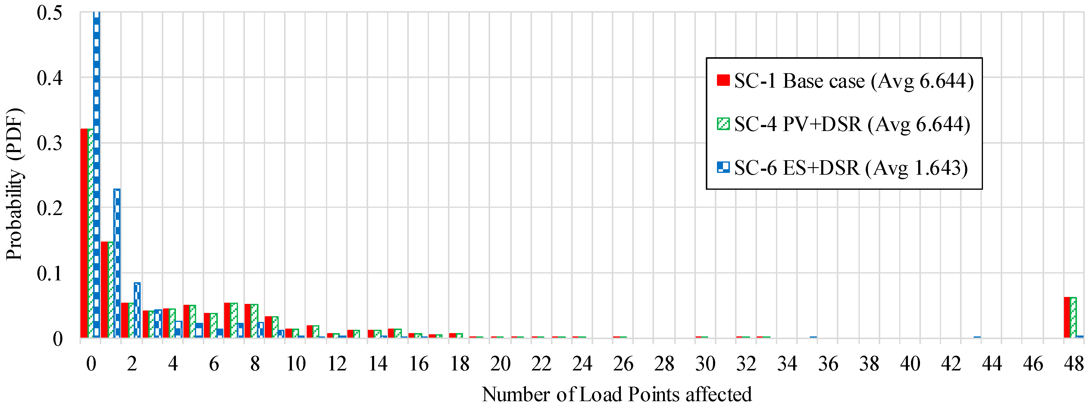
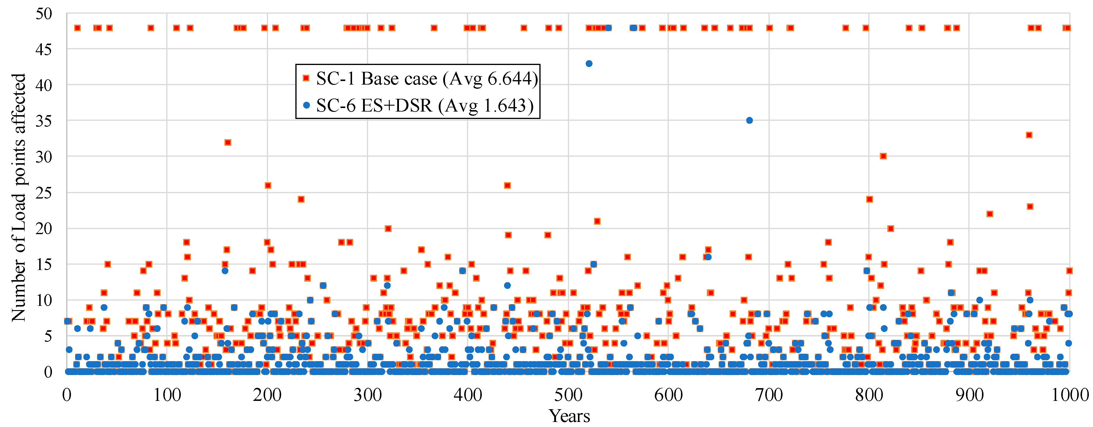
| Number of Load Points Affected | SC-1: Base Case | SC-4: PV + DSR | SC-6: ES + DSR | ||
|---|---|---|---|---|---|
| Probability | Probability | * | Probability | * | |
| 0 | 0.320 | 0.320 | 0% | 0.508 | −58.8% |
| 1 | 0.147 | 0.147 | 0% | 0.228 | −55.1% |
| 2–47 | 0.471 | 0.471 | 0% | 0.261 | 44.6% |
| 48 | 0.062 | 0.062 | 0% | 0.003 | 95.2% |
| ID | Scenario | SAIDI (hours/cust./y) | * | CAIDI (hours/cust. int.) | * | Average Duration of LI (hours) | * |
|---|---|---|---|---|---|---|---|
| SC-1 | Base case | 0.550 | - | 3.678 | - | 3.507 | - |
| SC-3 | PV | 0.453 | 17.7% | 3.043 | 17.3% | 2.888 | 17.7% |
| SC-4 | PV + DSR | 0.407 | 26.0% | 2.751 | 25.2% | 2.595 | 26.0% |
| SC-5 | ES | 0.310 | 43.7% | 6.172 | −67.8% | 1.975 | 43.7% |
| SC-6 | ES + DSR | 0.282 | 48.7% | 6.243 | −69.7% | 1.800 | 48.7% |
| ID | Scenario | ENS (kWh/c/y) | * | ACCI (kWh/Affected Customer) | * | Load Points Affected (avg) | * |
|---|---|---|---|---|---|---|---|
| SC-1 | Base case | 146.37 | - | 1090.41 | - | 6.644 | - |
| SC-3 | PV | 121.90 | 16.7% | 909.75 | 16.6% | 6.644 | 0% |
| SC-4 | PV + DSR | 110.63 | 24.4% | 828.99 | 24.0% | 6.644 | 0% |
| SC-5 | ES | 93.03 | 36.4% | 1793.87 | −64.5% | 1.841 | 72.3% |
| SC-6 | ES + DSR | 85.21 | 41.8% | 1790.79 | −64.2% | 1.643 | 75.3% |
© 2019 by the authors. Licensee MDPI, Basel, Switzerland. This article is an open access article distributed under the terms and conditions of the Creative Commons Attribution (CC BY) license (http://creativecommons.org/licenses/by/4.0/).
Share and Cite
Ndawula, M.B.; Djokic, S.Z.; Hernando-Gil, I. Reliability Enhancement in Power Networks under Uncertainty from Distributed Energy Resources. Energies 2019, 12, 531. https://doi.org/10.3390/en12030531
Ndawula MB, Djokic SZ, Hernando-Gil I. Reliability Enhancement in Power Networks under Uncertainty from Distributed Energy Resources. Energies. 2019; 12(3):531. https://doi.org/10.3390/en12030531
Chicago/Turabian StyleNdawula, Mike Brian, Sasa Z. Djokic, and Ignacio Hernando-Gil. 2019. "Reliability Enhancement in Power Networks under Uncertainty from Distributed Energy Resources" Energies 12, no. 3: 531. https://doi.org/10.3390/en12030531
APA StyleNdawula, M. B., Djokic, S. Z., & Hernando-Gil, I. (2019). Reliability Enhancement in Power Networks under Uncertainty from Distributed Energy Resources. Energies, 12(3), 531. https://doi.org/10.3390/en12030531