Article

Fault Simulation and Online Diagnosis of Blade Damage of Large-Scale Wind Turbines

School of Control and Computer Engineering, North China Electric Power University, Beijing 102206, China
*
Author to whom correspondence should be addressed.
Energies 2019, 12(3), 522; https://doi.org/10.3390/en12030522
Submission received: 23 December 2018 / Revised: 30 January 2019 / Accepted: 2 February 2019 / Published: 7 February 2019
(This article belongs to the Special Issue Maintenance Management of Wind Turbines)

Abstract

:
Damaged wind turbine (WT) blades have an imbalanced load and abnormal vibration, which affects their safe and stable operation or even results in blade rupture. To solve this problem, this study proposes a new method to detect damage in WT blades using wavelet packet energy spectrum analysis and operational modal analysis. First, a wavelet packet transform is used to analyze the tip displacement of the blades to obtain the energy spectrum. The damage is detected preliminarily based on the energy change in different frequency bands. Subsequently, an operational modal analysis method is used to obtain the modal parameters of the blade sections and the damage is located based on the modal strain energy change ratio (MSECR). Finally, the professional WT simulation software GH (Garrad Hassan) Bladed is used to simulate the blade damage and the results are verified by developing an online fault diagnosis platform integrated with MATLAB. The results show that the proposed method is able to diagnose and locate the damage accurately and provide a basis for further research of online damage diagnosis for WT blades.

1. Introduction

Blades are the most important component of a wind turbine (WT) and their operating status is an important factor to ensure the normal and stable operation of WTs. Since WTs are mostly located in harsh areas and the wind conditions are complex and changeable, blade faults occur more commonly with increasing operating hours. Blade faults manifest as blade damage and the reasons include fatigue due to alternating loads, lightning strokes, freezing and external impacts. If the damage is not detected and repaired in time, the blade will break or the WT may collapse and other serious accidents may occur. Therefore, online blade damage diagnosis is of great importance in terms of research value and applications [1].
The supervisory control and data acquisition (SCADA) information reflects the operating status of the WT and is easy to obtain. However, there are no data that directly reflect the state of the blades in the SCADA data. Therefore, it is important to investigate the health monitoring and fault diagnosis of the blades using intelligent algorithms such as artificial neural networks, expert systems, fuzzy logic systems and support vector machines and the WT SCADA data or vibration monitoring data. In Reference [2], a WT blade breakage monitoring method using SCADA data was proposed. A deep automatic coder (DA) model was proposed to determine impending blade damage from the SCADA data using a discriminant index. By analyzing fuzzy fault features, Yang et al. [3] detected blade faults by interpreting the data collected by the WT SCADA system; the authors used the conventional 10-minute average data in SCADA, which not only affected the diagnostic accuracy but also disregarded much of the fault training data [4].
On the other hand, it is more common to install sensors on the WT blades to monitor blade damage by using operational signals. The data directly reflect the structural damage to the blades and data processing is easy and the results are accurate. Therefore, much research has focused on the choice of sensors and signal processing. In Reference [5], an acoustic emission (AE) technique was used to obtain blade damage information and the location of the damage. Non-destructive AE methods were applied during a series of blade certification tests on a set of small WT blades [6]. However, the method requires the installation of an acoustic emitter and several receivers, which is technically difficult; in addition, the AE signals may suffer from interference from the signals from different blades or mechanical noise. In Reference [7,8], optical fiber sensors were embedded into WT blades and the blade damage was detected by processing the measured strain signal. However, optical fiber sensors can only be installed during blade manufacturing and this method is not suitable for WTs already in operation. A ceramic piezoelectric sensor mounted on the blades was used to perform a tensile test and a wavelet packet transform was used to diagnose and locate the damage [9]. Polyvinylidene fluoride resin (PVDF) film- based strain sensors were installed during a test of a full-scale WT [10]; the experimental results showed that the PVDF film-based sensors were effective for detecting damage at the trailing edge of the WT blade. In order to increase the accuracy of the damage diagnosis, the authors in Reference [11] used a hybrid sensor network consisting of capacitive film strain sensors and optical fiber sensors and using a sensor information fusion method based on a neural network. The above-mentioned experiments have achieved very good results and thin film sensors are easy to install; however, a sensor network consisting of a large number of sensors increases the installation difficulty and reduces the reliability of the system. Furthermore, it is still unknown whether the sensors affect the aerodynamic characteristics of the WT blades.
Vibration signal analysis is widely used in the field of mechanical fault diagnosis because it is a mature technology and vibration sensors are easy to install [12]. Therefore, vibration or acceleration sensors have been used commonly for damage diagnosis of blades. The authors in Reference [13,14,15] used the finite element analysis software ANSYS to simulate blade damage. The changes in the modal vibration shapes before and after blade damage were determined using vibration signal analysis. Because it is difficult to simulate WT operation processes in the ANSYS software, online blade damage diagnosis is not possible. However, the simulation results represent a good theoretical reference for damage diagnosis of blades using vibration sensors. In Reference [16], the characteristics of the vibration data before and after blade damage were determined under different environmental conditions and a principal component analysis was used for detecting the damage. Small-scale WT blades were used for damage experiments in Reference [17,18]. The change in the modal parameters was determined by analyzing the vibration signals of the blades. In Reference [19], a neural network was used to diagnose blade damage; the vibration signal data were obtained from excitation experiments. These types of methods are more common than simulation methods using ANSYS but they are still in the experimental stage. In many experiments, the vibration sensors were not actually installed on the blades. The use of a large number of sensors not only increases the installation difficulty but also affects the system reliability. In Reference [20], an exciter and several vibration sensors were installed on the blade of a Vestas V27 WT to monitor the operating conditions. This method was effective for monitoring the blade damage but requires an exciter for creating blade vibrations. In addition, harsh environmental conditions affect the reliability of the sensors.
In China, the most effective blade damage diagnosis method used in actual operations is still human observation. Therefore, a reliable and accurate method for online damage diagnosis is urgently needed. In this study, the GH Bladed software is used to simulate blade damage, which is then initially detected by analyzing the wavelet packet energy spectrum of the blade tip displacement. Unlike the SCADA system, Bladed is a reliable wind turbine simulation software that simulates blade faults accurately and obtains fault information without requiring a large amount of fault data. It has been shown that the wavelet packet method is more effective than the Fourier transform method. Moreover, the initial damage determination of the blades is also simpler and easier to implement using the wavelet packet decomposition method and the analysis does not complicate the diagnosis. When the blade is damaged, the modal parameters of the blade sections are determined using an operational modal analysis and subsequently, the modal strain energy (MSE) change ratio (MSECR) is calculated. The MSECR is used as an index to locate the damage. Computing the MSECR only requires the vibration signal of the blade, which can be measured by installing a small number of patch vibration sensors on the tip or embedding vibration sensors in the blade. Unlike acoustic emission technology and other methods of fault diagnosis that use sensors, an external signal excitation source does not have to be installed, which reduces the complexity and enhances the reliability of the system. Finally, a dynamic link library (DLL) is used to interface the Bladed and MATLAB software (2016a, MathWorks, Natick, MA, USA) to create an online diagnostic tool for WT blade damage. The simulation results show that this method can diagnose blade damage accurately. Moreover, the method can be applied to actual WTs by using a small number of patch-type vibration sensors on the blade tip.

2. Analysis and Simulation of Blade Damage Using GH Bladed

WT blades are typically constructed using fiber-reinforced polymeric composites and sandwich structures. Moreover, their geometries (e.g., the aerofoil chord length) gradually change along the pitch axis direction. It is, therefore, a challenging task to develop an accurate analytical model of the structural damage of WT blades. For simplification, in the present study, a WT blade is regarded as a multi-degree-of-freedom system consisting of 9 sections (U1–U9), as shown in Figure 1. The mass and stiffness can be adjusted in each section, as shown in Table 1.
Due to the large size and weight of large-scale WT blades, it is difficult to conduct damage experiments and the cost is high. GH Bladed provides a simulation platform that creates an approximation of an actual WT; the software contains a wealth of blade information, including length, thickness, stiffness, quality, airfoil and other data. It can also simulate the blade icing by setting the ice position and ice density. Therefore, it is convenient to use GH Bladed for fault analysis and diagnosis of blade icing. In some cases, blade icing and damage appear to be similar but the results are different. Blade icing mainly changes the quality of the blades. However, blade damage does not change the quality of blades but causes changes in the characteristic parameters such as blade stiffness. In addition, blade icing affects the operational parameters of the WT, such as the power and motor speed [21], whereas blade damage usually does not. Blade icing faults mostly occur in the cold season and cold regions and WT maintenance personnel detect blade icing using weather and WT SCADA data. Many studies have focused on blade icing diagnosis and deicing [22,23,24]. However, the connection between blade damage and weather is insignificant and there is no effective method for its detection.
In this study, we focus on changing the section stiffness and damping to simulate blade damage and we obtain the vibration information from GH Bladed. As the blade stiffness decreases, the vibration signal gradually increases along the major axis and the response is most pronounced at the tip of the blade. Therefore, the signal obtained from the tip is used for the initial damage detection of the blade damage. Figure 2 shows the vibration displacement of section 3, section 6 and the blade tip with severe damage in section 2; the simulation results demonstrate that the vibration signal increases gradually in the direction of the main axis. Figure 3 shows the blade tip displacement of a normal blade and a blade with severe damage.

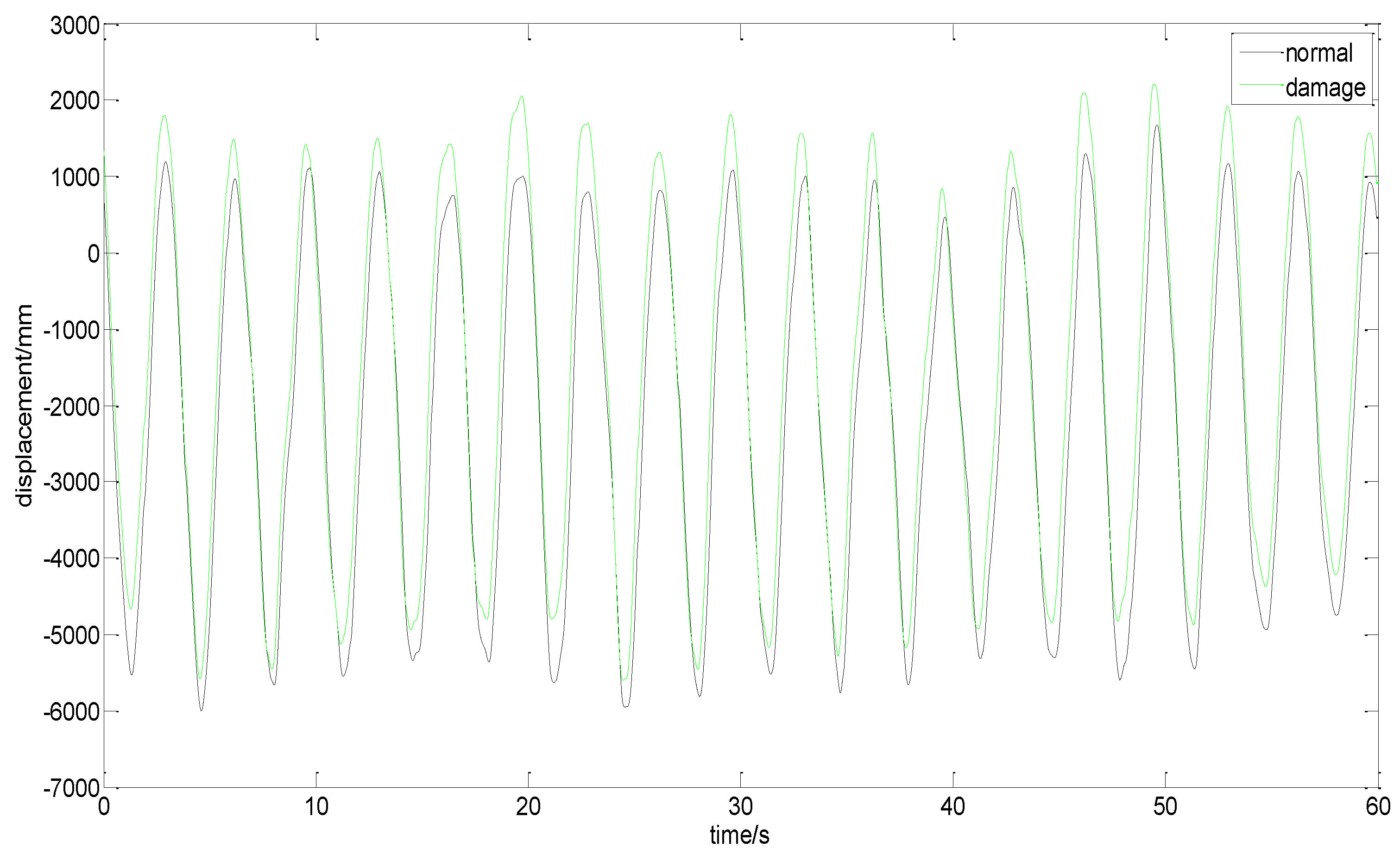
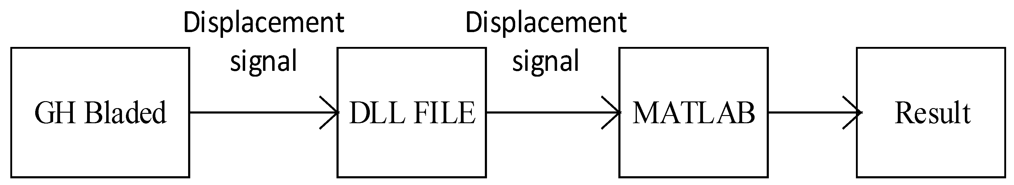
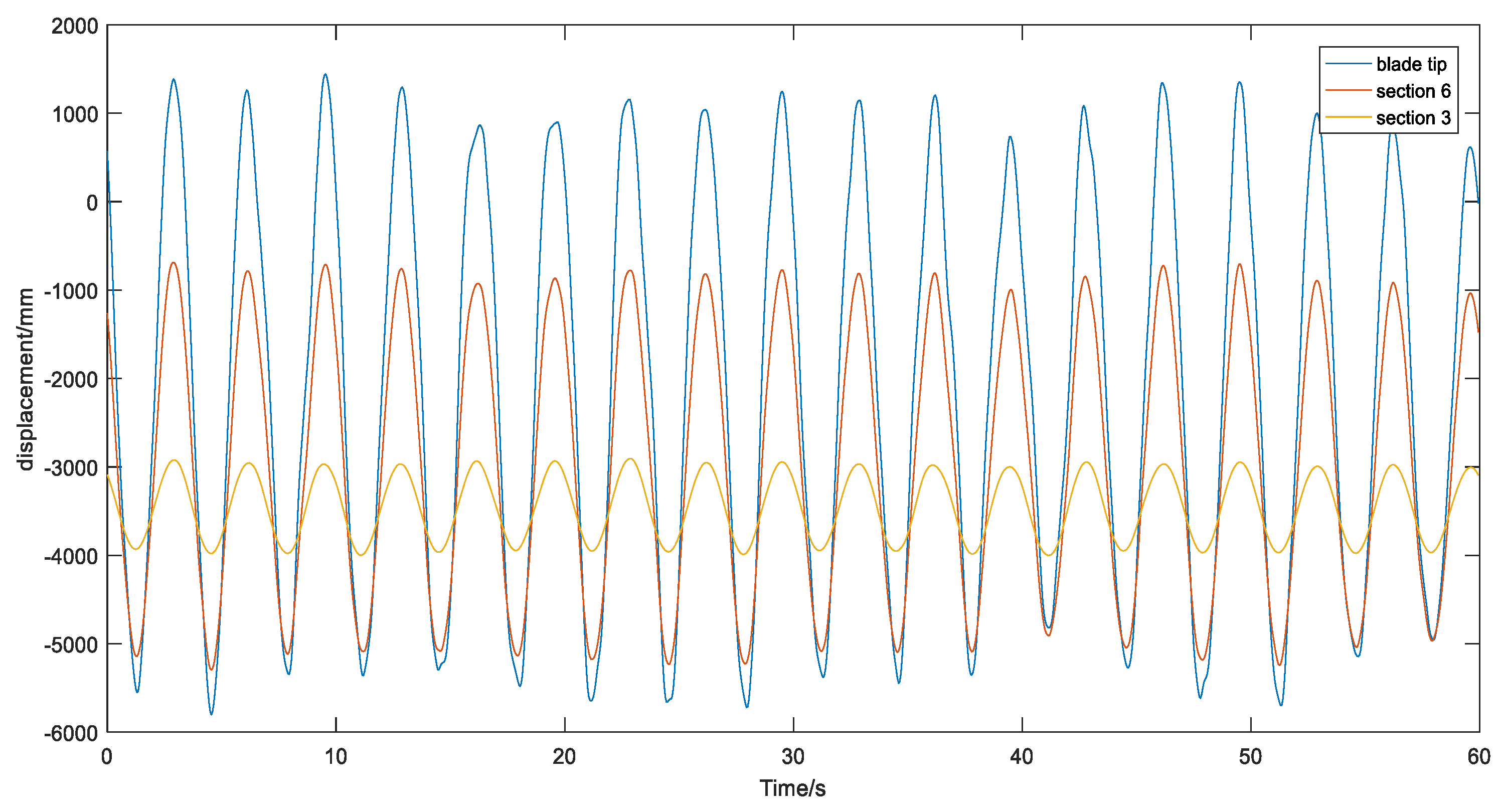
3. Signal Analysis of the Blade Tip Displacement

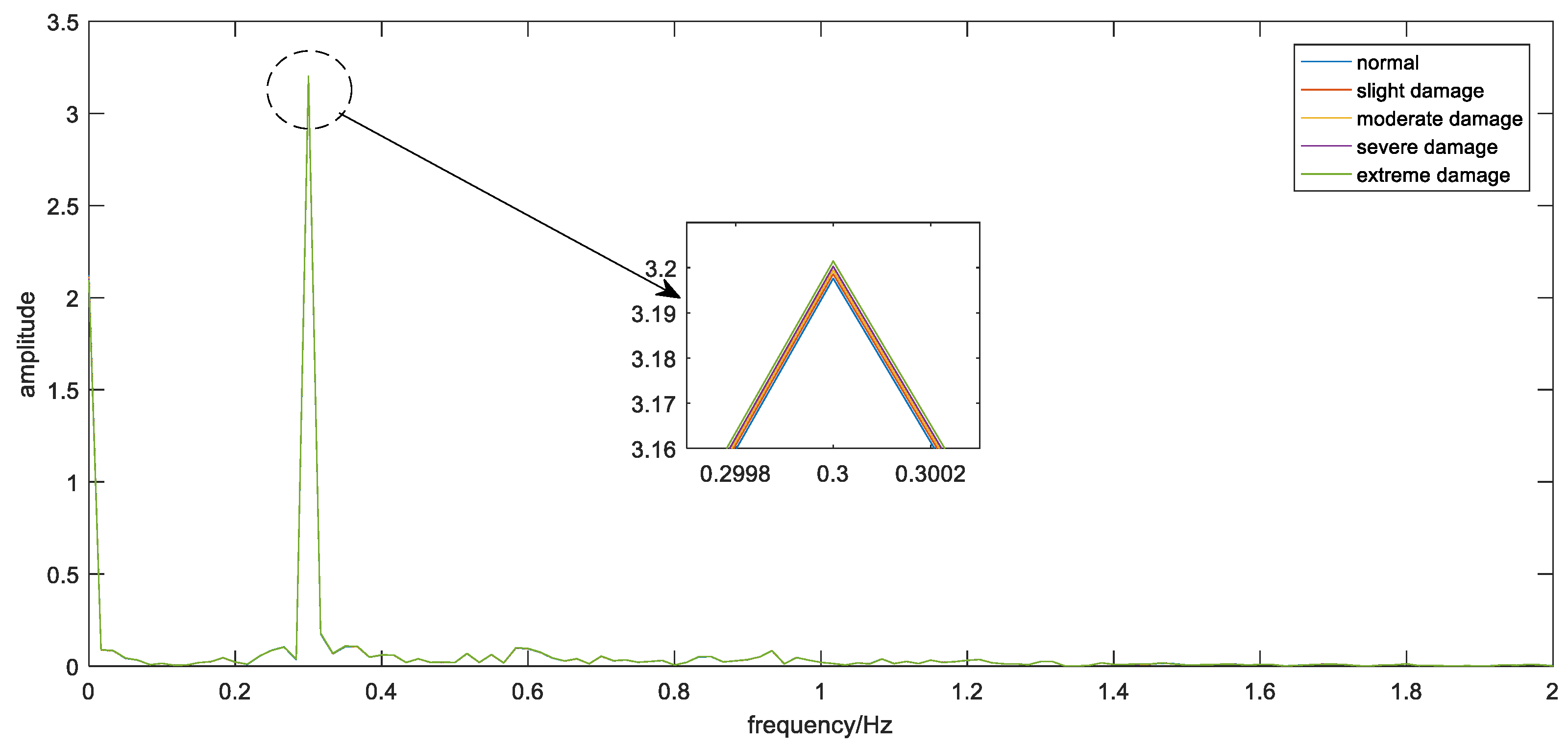
3.1. Fast Fourier Transform (FFT) Analysis of Blade Tip Displacement

Fourier analysis is commonly used in traditional signal analysis; it uses a fixed window function and does not reflect the non-stationary, time-domain and frequency-domain characteristics of the signals. Figure 4 shows the results of an FFT analysis of a blade tip displacement signal with different damage degrees in section 2. In the blade damage simulation, the blade parameters are assessed before and after the blade damage and the damage is divided into four classes, namely, slight damage, moderate damage, severe damage and extreme damage. For example, slight damage is defined as 80% of the original stiffness and moderate, severe and extreme damage are defined as 70%, 60% and 50% of the original stiffness, respectively. When there is little damage, the FFT of the blade tip displacement has no apparent influence on the low-frequency part and it is difficult to determine the blade damage using this method. The information in the high-frequency part is not accurate because of the limitations of the FFT analysis method. The wavelet transform is a method that uses a fixed area but a variable window size. Wavelet packet decomposition can adaptively select the frequency bands that match the signal spectrum based on certain signal characteristics [25].

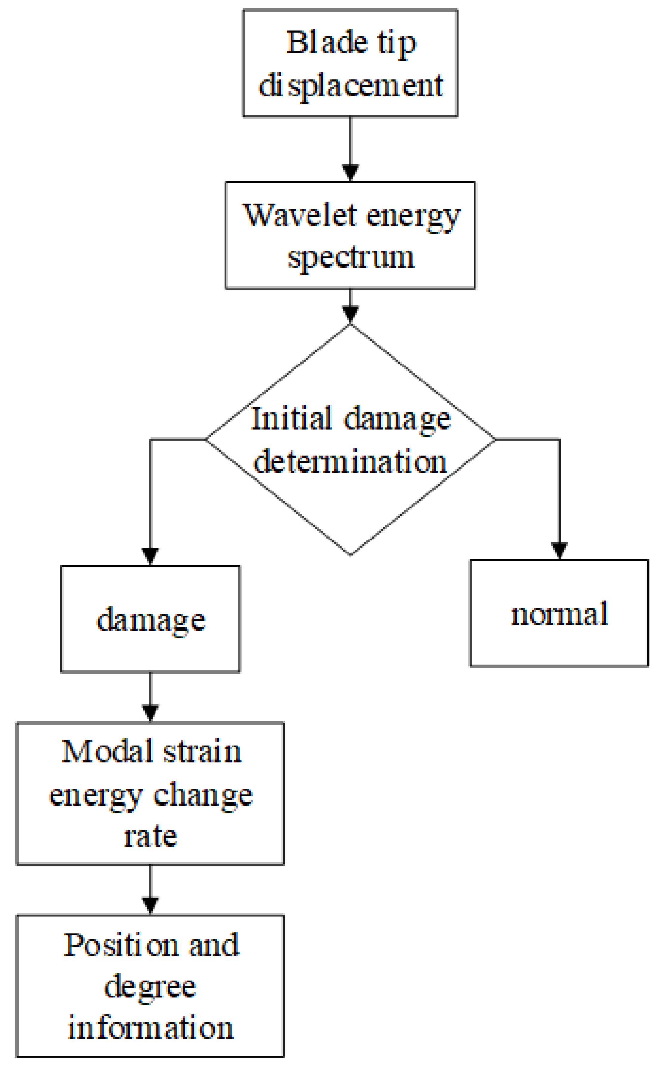
3.2. Wavelet Packet Energy Spectrum Extraction

A damaged blade exhibits abnormal vibration, which can be detected in the energy spectrum. The band energy reflects the operating status of the blade. By determining the change in the energy in different frequency bands, blade damage can be initially diagnosed. The energy-based wavelet packet decomposition results are called the wavelet packet energy spectrum of the blades.
We use a 3-layer wavelet packet decomposition as an example; the wavelet packet energy spectrum extraction method consists of the following steps:
(1) Obtaining the decomposition coefficients. The blade vibration signals are decomposed using a 3-layer wavelet packet decomposition; 8 decomposition coefficients of layer 3 from low frequency to high frequency are obtained ( X 3 0 , X 3 1 , X 3 2 , , X 3 7 ) .
(2) Reconstruction of the wavelet coefficients. We extract each sub-band range signal S 3 j ( j = 0 , 1 , , 7 ) ; the total signal is expressed as:
S = S 3 0 + S 3 1 + S 3 2 + + S 3 7
(3) Calculating the signal energy of each sub-band. The reconstructed signal of each layer 3 node is expressed as: S 3 j ( j = 0 , 1 , , 7 ) ; the corresponding band energy is E 3 j ( j = 0 , 1 , , 7 ) , which is defined as:
E 3 j = | S 3 j ( t ) | 2 d t = k = 1 N | x j k | 2
where x j k ( j = 0 , 1 , , 7 ; k = 0 , 1 , , n ) represents the amplitude of the signal’s discrete points.
The blade tip displacement signals were decomposed using the wavelet packet method to obtain the characteristic information of the tip displacement energy band. The details for the energy bands are shown in Table 2. The results show that the values of Band 1 increase with increasing degree of damage, although the differences are not large. The same is observed for the values of Bands 2 to 8 but the difference between the damaged blade and the normal blade is large enough to determine if the blade is damaged. Unlike the FFT analysis, this method has more significant eigenvalue changes and it is easier to determine the blade damage.
This method only requires vibration sensors at the blade tips to measure the displacement signal, which is easier to achieve than sensor installation and signal analysis for other kinds of sensors. If patch-type wireless sensors are used, there is less impact on the aerodynamic characteristics of the blade, making this method very suitable for blade health monitoring in currently used commercial WTs. Depending on the blade monitoring requirements, a number of sensors can be installed in different sections during blade manufacturing to detect the presence of damage and also the damage location. We report on the blade damage location using multi-sensor vibration signals in the next section of this paper.

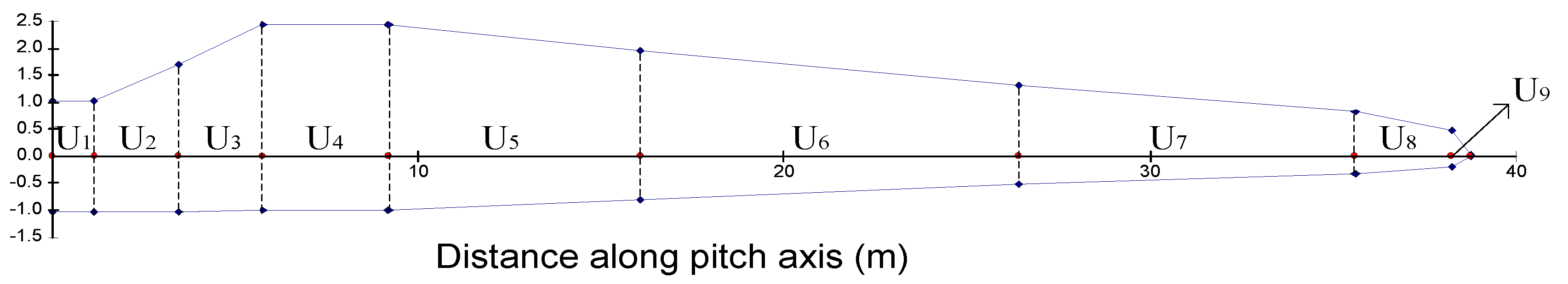
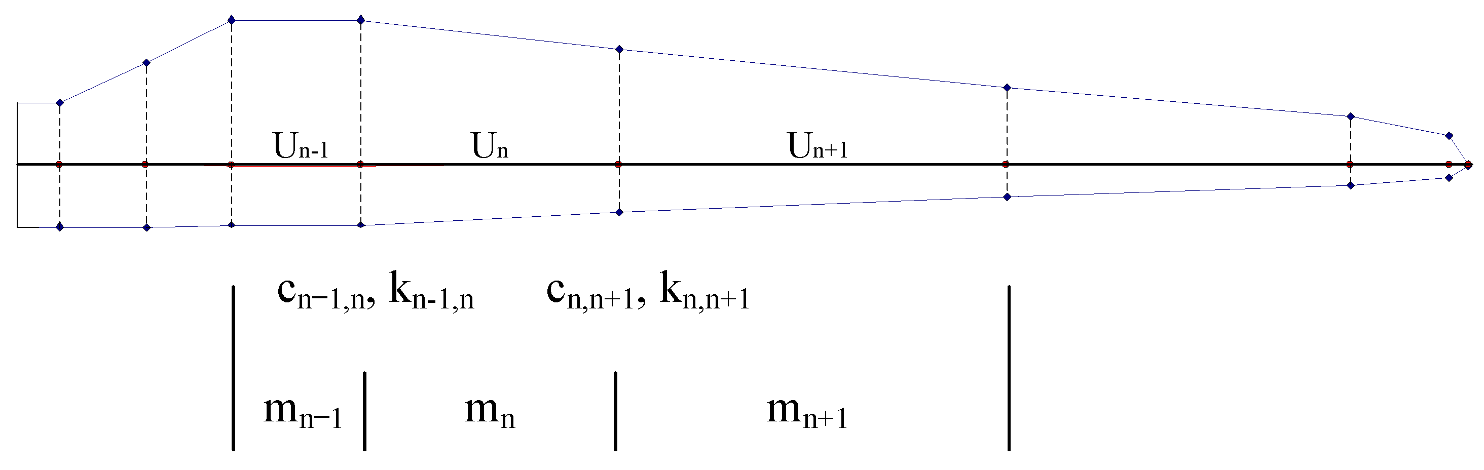
4. Blade Damage Location Based on Operational Modal Testing

In an experimental modal analysis, the modal parameters of a structure are obtained by the parameter identification of the system input and output signals collected under experimental conditions. Nevertheless, during the actual operation of a WT, no man-made excitation can be applied; therefore, an ambient excitation method is used, that is, the external wind condition is used as an excitation source. Subsequently, the operational mode test theory is applied to analyze the blade vibration signals. After a pretreatment using a random decrement technique, the output signal time series was analyzed using an autoregressive moving average (ARMA) model to solve for the modal parameters of each section. Finally, the blade damage location was determined by calculating the MSECR.

4.1. Operational Modal Test Method Applicable to WT Blades

The random decrement technique refers to removing or reducing random components from one or more stationary random response samples of a linear vibration system to obtain a free response signal under a certain initial excitation [26]. The following describes the basic principle of obtaining free vibration response signal data from a structure response signal using the random reduction method. For a linear system structure, the forced vibration response of a measuring point under any excitation can be expressed as:
y ( t ) = y ( 0 ) D ( t ) + y ˙ ( 0 ) V ( t ) + 0 t h ( t τ ) f ( τ ) d τ
where D(t) is the free vibration response at an initial displacement of 1 and an initial velocity of 0. V(t) is the free vibration response at an initial displacement of 1 and initial velocity of 0. y(0) is the initial displacement and y ˙ ( 0 ) is the initial velocity of the system vibration. h(t) is the system unit impulse response function. f (t) is the external excitation. We selected a suitable constant A to intercept a measured random vibration structure response signal y(t); a series of different intersection moments ti (i = 1, 2, ..., N) can be obtained and the response y(tti) from the moment ti can be seen as a linear superposition of three parts: the free vibration response caused by the initial displacement at ti, the free vibration response caused by the initial velocity at ti and the forced vibration response caused by the random excitation f(t). Therefore:
y ( t t i ) = y ( t i ) D ( t t i ) + y ˙ ( t i ) V ( t t i ) + t i t h ( t τ ) f ( τ ) d τ
Since the excitation f(t) is stationary and the starting point does not affect its random characteristics, a series of starting points ti of y(tti) can be moved to coordinate the origin to obtain the subsample function xi(t) (i = 1, 2, ..., N). That is:
x i ( t ) = A D ( t ) + y ˙ ( t i ) V ( t ) + 0 t h ( t τ ) f ( τ ) d τ
The statistical average of xi(t) is:
  x ( t ) = 1 N i = 1 N X i ( t ) E [ A D ( t ) + y ˙ ( t i ) V ( t ) + 0 t h ( t τ ) f ( τ ) d τ ]                     A D ( t ) + E [ y ˙ ( t i ) ] V ( t ) + 0 t h ( t τ ) E [ f ( τ ) ] d τ
If the excitation f(t) is a stationary pure random vibration with a mean value of 0 and the system vibration response y(t) and y ˙ ( t i ) is also a stationary random vibration with a mean of 0, then:
E [ f ( t ) ] = 0 E [ y ˙ ( t i ) ] = 0
According to the above:
x ( t ) A D ( t )
where x(t) is called the free vibration response obtained by the random decrement method. Generally, turbulent wind is a natural random excitation in WTs and the mean vibration velocity of a blade tip should be zero, that is, E [ y ˙ ( t i ) ] is zero. However, the mean value response of the blade tip displacement is not zero; therefore, the random decrement method cannot be directly applied to the original tip displacement signal [27]. Under the excitation of an average wind speed, the tip displacement is:
0 t h ( t τ ) E [ f ( τ ) ] d τ = 0 t h ( t τ ) g ( v ¯ ) d τ = B
where v ¯ is the average wind speed from time 0 to t, B is the mean value of the blade tip displacement,   g ( v ¯ ) is the blade excitation function for a wind speed of v ¯ . In order to ensure that this method is applicable to the tip displacement signal, the signal should be pre-processed by subtracting the mean value B so that the mean value is zero. Therefore:
x ( t ) = 1 N i = 1 N [ X i ( t ) B ] E [ A D ( t ) + y ˙ ( t i ) V ( t ) ] = A D ( t )
According to Equation (10), a free vibration response with an initial displacement of A and an initial velocity of 0 is obtained. The response is determined by using an ARMA model time series analysis, which is a method of using parametric models to process ordered random vibration response data for modal parameter identification [28]. The relationship between the linear system excitation and the response for N degrees of freedom can be described by a higher-order differential equation, which becomes a differential equation represented by several time series at different times, the ARMA temporal model equation, in a discrete time domain:
k = 0 2 N a k x t k = k = 0 2 N b k f t k
Equation (11) describes the relationship between the response data sequence xt and the historical value xt−k, where 2N is the order of the autoregressive model and the sliding mean model, ak, bk denote the autoregressive coefficient and the sliding mean coefficient to be identified respectively and ft denotes white noise excitation. When k = 0, let a0 = b0 = 1. The ARMA equation {xt} has a unique smooth solution:
x t = i = 0 h t f t i
where ht is the impulse response function and ft is white noise. Therefore:
E [ f t i f t + τ k ] = { σ 2 ( k = τ + i ) 0 ( o t h e r s )
where δ2 is the white noise variance. By substituting the result of Equation (13) into Equation (12), the following is obtained:
R τ = σ 2 i = 0 h i h i + τ
Since the linear system impulse response function ht is the system output response when excited by a pulse signal δt, the expression defined by the ARMA process is:
k = 0 2 N a k h t k = k = 0 2 N b k σ t k = b t
After calculating the autoregressive coefficient ak and the sliding mean coefficient bk, the system modal parameters can be calculated by using the expression of the ARMA model transfer function:
H ( z ) = k = 0 2 N b k z k k = 0 2 N a k z k
The root of the denominator polynomial equation is solved using a high-order algebraic equation solving method and the obtained root is the pole of the transfer function. Their relationship with the system modal frequency ωk and the damping ratio ξk is:
{ z k = e s k Δ t = e ( ξ k ω k + j ω k 1 ξ k 2 ) Δ t z k * = e s k * Δ t = e ( ξ k ω k j ω k 1 ξ k 2 ) Δ t
The modal frequency ωk and the damping ratio ξk can be obtained from Equation (18), that is:
{ R k = ln z k = s k Δ t ω k = | R k | Δ t ξ k = 1 1 + ( I m ( R k ) R e ( R k ) ) 2
Suppose that the k-order residue of Hpq (s), which is the transfer function of the p-point response excited at point q, is Akpq, then the residue can be calculated as follows:
A k p q = l i m z z k H p q ( z ) ( z z k ) = k = 0 2 N b k z k k = 0 2 N a k z k ( z z k ) | z = z k
The modal vector can be obtained by processing the residue obtained from a series of measured response points. For a structure with n response points, the first task is determining the measurement point with the largest absolute value from the residue of n corresponding modes of the same order. Assuming that the point is the measurement point m, the normalized complex modal vector corresponding to the k-order mode can be obtained by the following formula:
{ ϕ k } = [ A K 1 q A k 2 q   A k m q ] T / A k m q
In this way, the modal parameters such as the modal frequency, modal damping and modal vibration mode can be obtained.

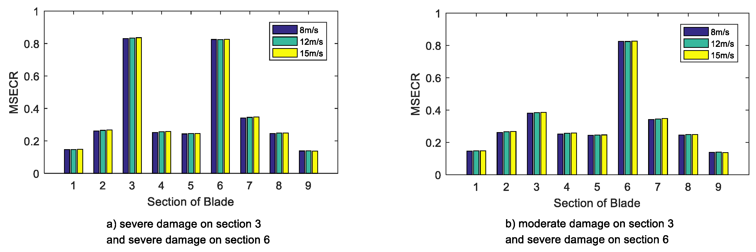
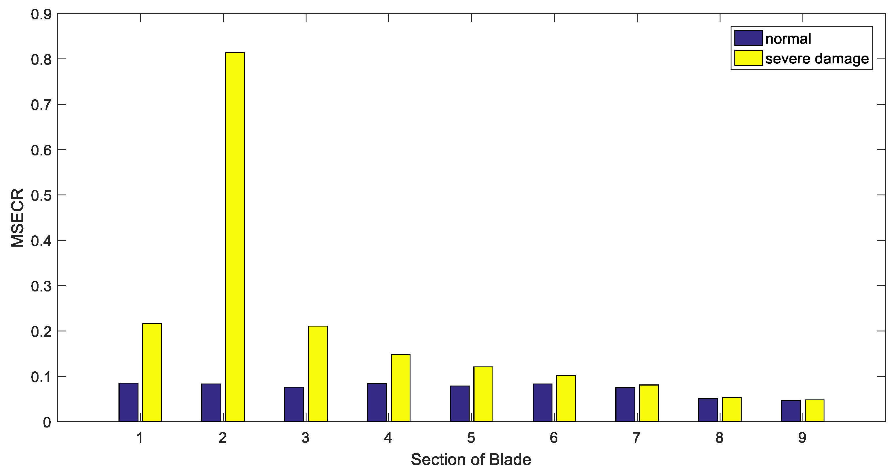
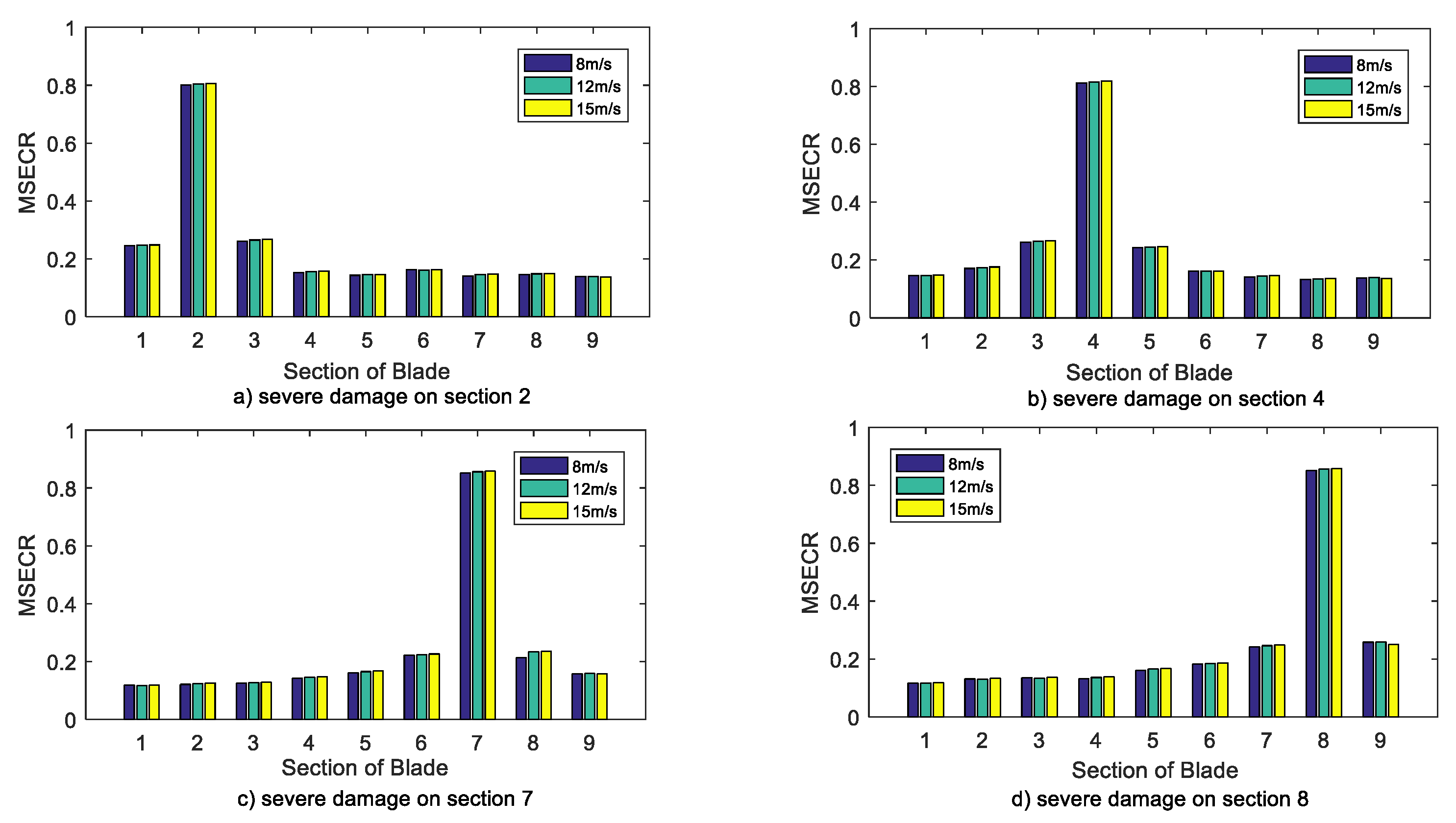
4.2. Blade Damage Location Analysis Based on the MSECR

Because a blade can be simplified as a hollow cantilever beam structure, a model of the blade sections was developed based on the structural characteristics and material properties (Figure 5). Three neighboring sections are denoted as Un−1, Un and Un+1 with the masses of mn−1, mn and mn+1, respectively. The sections Un−1 and Un are connected via stiffness kn−1,n and damping cn−1,n and the sections Un and Un+1 are connected via kn,n+1 and cn,n+1. Consequently, when an external load is applied to the blade, the dynamic response can be expressed by the following equation:
M x ¨ + C x ˙ + K x = F ( t )
where x represents the vector of the displacement responses along the blade; M, C and K denote the equivalent structural mass, the equivalent structural damping and the equivalent structural stiffness matrices, respectively; F is the matrix of the external forces. It can be inferred that when a local defect occurs in section n, the values of cn−1,n, cn,n+1, kn−1,n and kn,n+1 change correspondingly, whereas the damping and stiffness in the other sections may not change.
This configuration was the inspiration for developing a damage location diagnosis method for WT blades using the modal analysis of the sections. Blade icing has a significant influence on the mass characteristic parameters of the blade but has little effect on stiffness and damping. Since the values of the damping and stiffness are dependent only on the blade’s structural integrity, the proposed damage location diagnosis method responds only to changes caused by structural damage. Therefore, false alarms due to ice on the blade surfaces can be avoided.
The damage to the blade structure has nothing to do with its mass, that is to say, [ Δ M ] = 0 . Therefore, structural damage is equivalent to a change in stiffness. Equation (22) shows the relationship between the structural stiffness and the modal vibration modes before and after the damage has occurred (superscript d indicates the damaged section):
[ K d ] = [ K ] + [ Δ K ] = [ K ] + j = 1 L j [ K j ] { ϕ i d } = { ϕ i } + { Δ ϕ i } = { ϕ i } + j = 1 n c i j { ϕ j }
In Equation (22), 1 < j < 0 and 0 < c i j < 1 . In addition, the MSE is related to the mode shape. The i-order MSE of the j-th section before and after structural damage is defined as follows:
M S E i j = { ϕ i } T [ K j ] { ϕ i } M S E i j d = { ϕ i d } T [ K j ] { ϕ i d }
Usually, only a low-order modal term is calculated and the high-order modal terms are ignored; the MSE of the section before and after structural damage is defined as follows:
M S E C i j = M S E i j d M S E i j = 2 { ϕ i } T [ K j ] { Δ ϕ i }
This analysis indicates that the damage location can be diagnosed by the index vectors obtained from the MSE. However, this is not sufficient to determine the damage degree. The MSECR is defined as the indicator of the damage degree:
M S E C R i j = | M S E i j d M S E i j | M S E i j
where MSECRij is the MSECR for the j-th section with respect to the i-order mode.
In order to reduce the influence of the experimental modal random noise, multiple different order modalities can be used to diagnose the location of structural damage.
M S E C R j = 1 m i = 1 m M S E C R i j M S E C R i m a x
where m is the number of used modalities and MSECRimax is the maximum MSECR [25].
The theoretical analysis shows that when the change in the stiffness matrix and the modal parameters before and after structural damage are used as input diagnostic information, the location of the blade damage can be obtained using the MSECR.

5. Simulation Verification

The GH Bladed software possesses high-precision WT modeling and simulation functions but the data post-processing capability is limited. In contrast, the MATLAB software has strong data analysis and post-processing capability and a rich algorithm toolbox. However, the nonlinear model of the WT created in MATLAB has low accuracy and the simulation function is also very limited. In order to verify the proposed series of blade damage diagnosis methods and perform online diagnostic simulation, the two software applications have to be combined into a fault simulation platform. Because there is no direct data communication interface between the two applications, the data interaction between GH Bladed and MATLAB was implemented by using the Bladed external DLL interface file. The schematic diagram of the integration is shown in Figure 6. The fault data were exported to MATLAB through the DLL file and the signal analysis and damage diagnosis were performed. Because the Bladed external DLL data interface allows for setting a data transmission time interval, the data transmission mode is very similar to the data acquisition process between the SCADA system and the actual sensors. Moreover, Bladed has a sensor simulation function, in which the sensor characteristics such as the signal noise, delay and fault can be specified. This greatly increases the simulation accuracy and credibility of the online monitoring and diagnosis simulation performed in this study.
The experimental WT data used in GH Bladed are shown in Table 3. Figure 6 shows the flowchart of the blade damage diagnosis. The specific steps were as follows: First, the wavelet packet decomposition of the blade tip displacement signal was conducted to obtain the characteristic information of the energy bands. The blade damage was preliminarily determined based on these characteristics. For the damaged blade, the modal parameters of each section were calculated using the operational modal method and the MSECR was obtained. The MSECR represented the index to determine the location of the damage.
When the wavelet packet energy of the blade tip displacement signals is abnormal, the displacement signals of each section are analyzed using the operational modal analysis method to obtain the modal parameters of every section and the MSECR. Figure 7 shows the flowchart of the blade damage diagnosis. Table 4 shows the modal parameters of section 2 with severe damage. The MSECR was calculated using the data in Table 4 and the damage location was determined using MSECR as the discriminant index. Figure 8 shows the MSECR histograms of section 2 before and after the severe damage occurred at a mean wind speed of 12 m/s.
In order to further illustrate the effectiveness of this method, a large number of simulation experiments were conducted using blade damage in different locations and different degrees of damage. Figure 9 shows the MSECR histograms for the different locations and degrees of damage for different wind speeds. The blade damage location can be clearly detected in Figure 9. Figure 10 shows the MSECR histograms of when two sections were damaged.
Figure 9 shows the MSECR of each blade section when a single section is damaged. The simulation results show that the MSECR of the damaged section has a prominent peak, which is significantly higher than those of the undamaged sections. The MSECR of the damage section in Figure 9 is about five times as large as those of the normal sections. In addition, the MSECRs of the adjacent sections were also slightly higher than (about 50% higher than the normal sections) and there was no significant change in the MSECR of the distant sections. Therefore, the damaged section can be determined based on the MSECR. Figure 10 shows the MSECR of each blade section when two sections are damaged. It is observed that the MSECR of the damaged section is higher than that of the normal section. It is noteworthy that the MSECR provided a good indication of the degree of damage if the damage degree of the two damaged sections was large (as shown in Figure 10a). However, when the damage degree was significantly different for the two sections, the sections with the smaller damage sections may be difficult to detect (as shown in Figure 10b). As a result, it is possible to miss some minor damage when using this method for blade damage location but this does not affect the diagnosis and location of the major damage when the blade is damaged in multiple sections. Generally, blade damage consists mostly of single-section damage. And the more serious parts should be mainly considered in multiple-section damage. Environmental conditions affect the structural characteristics of the blade and the calculated value of the wavelet energy spectrum will differ under different weather conditions; however, the location of the damage is not affected. Therefore, this method can be used to locate blade damage effectively.

6. Conclusions

The proposed method for blade damage diagnosis and damage location based on the tip displacement signal, wavelet packet decomposition and operational modal analysis has the following characteristics:
(1) The wind power simulation software Bladed was used to simulate the blade damage fault of a wind turbine by determining the change in the structural characteristic parameters before and after blade damage. An integrated MATLAB and Blade simulation platform was developed for real-time online damage diagnosis.
(2) An initial on-line blade damage assessment was conducted using Fourier analysis and wavelet packet energy spectrum analysis of the tip displacement. The simulation results showed that the wavelet packet energy spectrum analysis was not only easy to implement but also provided significantly better results than the traditional Fourier analysis.
(3) A method for identifying the working modal parameters of the blades was proposed by combining the random decrement method and ARMA model parameter identification. The damage was accurately located by calculating the MSECR of each blade section without requiring additional excitation signals and the method proved effective for different degrees of damage occurring simultaneously.
Although the results of this study are based on software simulation results, the Blade software provides high accuracy and is suitable for preliminary assessment prior to empirical research. In a future study, we will build a small-blade experimental wind turbine and develop a wireless patch sensor for empirical research. The results of this study provide methodological guidance for system implementation.

Author Contributions

Conceptualization, F.G.; methodology, F.G and Q.L.; software, X.Y. and X.W.; validation, J.L. and X.W.; writing—original draft preparation, Q.L.; writing—review and editing, X.W.

Funding

The authors would like to acknowledge the funding support from the National Nature Science Fund Project (51677067).

Conflicts of Interest

The authors declare no conflict of interest.

References

  1. Yang, B.; Sun, D. Testing, inspecting and monitoring technologies for wind turbine blades: A survey. Renew. Sustain. Energy Rev. 2013, 22, 515–526. [Google Scholar] [CrossRef]
  2. Wang, L.; Zhang, Z.; Xu, J.; Liu, R. Wind turbine Blade Breakage Monitoring with Deep Auto encoders. IEEE Trans. Smart Grid 2018, 9, 2824–2833. [Google Scholar] [CrossRef]
  3. Yang, W.; Court, R.; Jiang, J. Wind turbine condition monitoring by the approach of SCADA data analysis. Renew. Energy 2013, 53, 365–376. [Google Scholar] [CrossRef]
  4. Helbing, G.; Ritter, M. Deep learning for fault detection in wind turbines. Renew. Sustain. Energy Rev. 2018, 98, 189–198. [Google Scholar] [CrossRef]
  5. Tang, J.; Soua, S.; Mares, C.; Gan, T.H. An experimental study of acoustic emission methodology for inservice condition monitoring of wind turbine blades. Renew. Energy 2016, 99, 170–179. [Google Scholar] [CrossRef]
  6. Joosse, P.A.; Blanch, M.J.; Dutton, A.G.; Kouroussis, D.A.; Philippidis, T.P.; Vionis, P.S. Acoustic emission monitoring of small wind turbine blades. J. Sol. Energy Eng. 2002, 124, 446–454. [Google Scholar] [CrossRef]
  7. Sierra-Pérez, J.; Torres-Arredondo, M.A.; Güemes, A. Damage and nonlinearities detection in wind turbine blades based on strain field pattern recognition. FBGs, OBR and strain gauges comparison. Compos. Struct. 2016, 135, 156–166. [Google Scholar] [CrossRef]
  8. Oh, K.Y.; Park, J.Y.; Lee, J.S.; Epureanu, B.I.; Lee, J.K. A Novel Method and Its Field Tests for Monitoring and Diagnosing Blade Health for WTs. IEEE Trans. Instrum. Meas. 2015, 64, 1726–1733. [Google Scholar]
  9. Ruan, J.; Ho, S.C.; Patil, D.; Song, G. Structural Health Monitoring of wind turbine Blade using Piezo ceremic Based Active Sensing and Impedance Sensing. In Proceedings of the 11th IEEE International Conference on Networking, Sensing and Control, Miami, FL, USA, 7–9 April 2014; Volume 64, pp. 661–666. [Google Scholar]
  10. Huh, Y.H.; Kim, J.I.; Lee, J.H.; Hong, S.G.; Park, J.H. Application of PVDF Film Sensor to Detect Early Damage in wind turbine Blade Components. Procedia Eng. 2011, 10, 3304–3309. [Google Scholar] [CrossRef]
  11. Downey, A.; Ubertini, F.; Laflamme, S. Algorithm for damage detection in wind turbine blades using a hybrid dense sensor network with feature level data fusion. J. Wind Eng. Ind. Aerodyn. 2017, 168, 288–296. [Google Scholar] [CrossRef] [Green Version]
  12. Sarrafi, A.; Mao, Z.; Niezrecki, C.; Poozesh, P. Vibration-based damage detection in wind turbine blades using Phase-based Motion Estimation and motion magnification. J. Sound Vib. 2018, 421, 300–318. [Google Scholar] [CrossRef] [Green Version]
  13. Rezaei, M.M.; Behzad, M.; Moradi, H.; Haddadpour, H. Modal-based damage identification for the nonlinear model of modern wind turbine blade. Renew. Energy 2016, 94, 391–409. [Google Scholar] [CrossRef]
  14. Moradi, M.; Sivoththaman, S. MEMS Multi sensor Intelligent Damage Detection for wind turbines. IEEE Sens. J. 2015, 15, 1437–1444. [Google Scholar] [CrossRef]
  15. Abouhnik, A.; Albarbar, A. Wind turbine blades condition assessment based on vibration measurements and the level of an empirically decomposed feature. Energy Convers. Manag. 2012, 64, 606–613. [Google Scholar] [CrossRef]
  16. Gonzalez, A.G.; Fassois, S.D. A supervised vibration-based statistical methodology for damage detection under varying environmental conditions & its laboratory assessment with a scale wind turbine blade. J. Sound Vib. 2016, 366, 484–500. [Google Scholar]
  17. Wang, Y.; Liang, M.; Xiang, J. Damage detection method for wind turbine blades based on dynamics analysis and mode shape difference curvature information. Mech. Syst. Signal Process. 2014, 48, 351–367. [Google Scholar] [CrossRef]
  18. Lee, K.; Aihara, A.; Puntsagdash, G.; Kawaguchi, T.; Sakamoto, H.; Okuma, M. Feasibility study on a strain based deflection monitoring system for wind turbine blades. Mech. Syst. Signal Process. 2017, 82, 117–129. [Google Scholar] [CrossRef]
  19. Dervilis, N.; Choi, M.; Taylor, S.G.; Barthorpe, R.J.; Park, G.; Farrar, C.R.; Worden, K. On damage diagnosis for a wind turbine blade using pattern recognition. J. Sound Vib. 2014, 333, 1833–1850. [Google Scholar] [CrossRef]
  20. Tcherniak, D.; Molgaard, L.L. Active vibration-based structural health monitoring system for wind turbine blade: Demonstration on an operating Vestas V27 WT. Struct. Health Monit. 2017, 16, 536–550. [Google Scholar] [CrossRef]
  21. Shu, L.; Li, H.; Hu, Q.; Jiang, X.; Qiu, G.; McClure, G.; Yang, H. Study of ice accretion feature and power characteristics of wind turbines at natural icing environment. Cold Reg. Sci. Technol. 2018, 147, 45–54. [Google Scholar] [CrossRef]
  22. Saleh, S.A.; Moloney, C.R. Development and testing of wavelet packet transform-based detector for ice accretion on wind turbines. In Proceedings of the 2011 Digital Signal Processing and Signal Processing Education Meeting (DSP/SPE), Sedona, AZ, USA, 4–7 January 2011; pp. 72–77. [Google Scholar]
  23. Li, Y.; Wang, S.; Liu, Q.; Feng, F.; Tagawa, K. Characteristics of ice accretions on blade of the straight-bladed vertical axis wind turbine rotating at low tip speed ratio. Cold Reg. Sci. Technol. 2017, 145, 1–13. [Google Scholar] [CrossRef]
  24. Corradini, M.L.; Ippoliti, G.; Orlando, G. A Sliding Mode Observer-Based Icing Detection and Estimation Scheme for Wind Turbines. J. Dyn. Syst. Meas. Control 2018, 140, 014502. [Google Scholar] [CrossRef]
  25. Liu, T.; Li, A.Q.; Ding, Y.L.; Li, Z.J.; Fei, Q.G. Experimental study on structural damage alarming method based on wavelet packet energy spectrum. J. Vib. Shock 2009, 28, 4–9. [Google Scholar]
  26. Luo, J.; Liu, G.; Huang, Z.-M. Modal parametric identification under non-stationary excitation based on random decrement method. J. Vib. Shock 2015, 21, 19–24. [Google Scholar]
  27. Zhao, Y.; Xue, B.; Zhang, J.; North China University of Water Resources and Electric Power. Research on Modal Parameter Identification of Bridge Structure Based on ARMA Model. J. North China Univ. Water Resour. Electr. Power 2015, 36, 21–24. [Google Scholar]
  28. Seyedpoor, S.M. A two stage method for structural damage detection using modal strain energy based index and particle swarm optimization. Int. J. Non-Linear Mech. 2012, 47, 1–8. [Google Scholar] [CrossRef]
Figure 1. Blade section settings in the GH (Garrad Hassan) Bladed software
Energies 12 00522 g001
Figure 2. Displacement signal of different sections when section 2 is damaged.
Energies 12 00522 g002
Figure 3. Blade tip displacement of normal and damaged blades.
Energies 12 00522 g003
Figure 4. FFT analysis of blade tip displacement with different damage degree.
Energies 12 00522 g004
Figure 5. Model of the blade sections.
Energies 12 00522 g005
Figure 6. Flowchart of the integration of the Bladed and MATLAB data.
Energies 12 00522 g006
Figure 7. Flowchart of the blade damage diagnosis.
Energies 12 00522 g007
Figure 8. The MSECR of section 2 before and after damage.
Energies 12 00522 g008
Figure 9. MSECR histograms for damage in one section.
Energies 12 00522 g009
Figure 10. MSECR histograms for damage in two sections.
Energies 12 00522 g010
Table 1. Blade geometry and mass/stiffness information.
Section12345678910
Distance along pitch axis (m)01.153.445.749.1916.0726.4135.5938.2338.75
Chord (m)2.072.072.763.443.442.761.841.150.690.03
Aerodynamic twist (deg)00913117.83.30.32.754
Thickness (%)1001006440302215131313
Mass/unit length(kg/m)1084.77369.81277.36234.21209.56172.58103.5555.4740.6824.65
Edgewise stiffness (N·m2)7.47 × 1092.61 × 1092.09 × 1091.43 × 1091.29 × 1095.65 × 1081.22 × 1082.43 × 1074,518,0008167.51
Flapwise stiffness (N·m2)7.47 × 1092.43 × 1091.41 × 1098.34 × 1085.56 × 1082.09 × 1082.95 × 1072,259,000113,8243127.98
Table 2. Tip displacement energy spectrum data.
Damage DegreeBand 1Band 2Band 3Band 4Band 5Band 6Band 7Band 8
Extreme damage94.85252.11980.56380.11490.05850.02590.01390.0043
Severe damage94.71382.11730.56340.11480.05850.02590.01390.0043
Moderate damage94.63682.11260.56310.11460.05850.02580.01390.0044
Slight damage94.56332.12030.55730.11410.05840.02580.01380.0043
Normal94.294615.70021.86777.70630.41630.32630.90873.8432
Table 3. Parameters of the experimental WT.
NumberParameter NameValue
1Length of blade38.75 m
2Rated wind speed12 m/s
3Rated power2 WM
4Above-rated generator speed set-point1500 rpm
5Transmission ratio83.33
6Minimum generator speed850 rpm
7Pitch angle range−2–90°
8Height of tower60 m
9Rated generator torque13,403 Nm
10Maximum generator torque14,400 Nm
11Air density1.225 kg/m3
12Cut-in wind speed4 m/s
13Cut-out wind speed25 m/s
14Number of blades3
15Rotor diameter80 m
Table 4. Modal parameters of each unit.
Blade UnitFirst-Order FrequencyFirst-Order ModeSecond-Order FrequencySecond-Order Mode
10.3201−0.0052073.83430.000059
20.2986−0.0028343.7893−0.000078
30.27940.0173483.9138−0.000144
40.26770.0732194.08170.000130
50.24720.3042024.3765−0.000204
60.20361.4193674.3478−0.001643
70.23491.0963823.3818−0.030174
80.24451.0433853.0982−0.011586
90.24641.0267993.1026−0.013261

