Online Diagnosis of Inter-turn Short Circuit for Dual-Redundancy Permanent Magnet Synchronous Motor Based on Reactive Power Difference

Abstract

The Dual-Redundancy Permanent Magnet Synchronous Motor (DRPMSM) with weak thermal coupling and no electromagnetic coupling among phase windings has two sets of three-phase symmetrical windings. Under normal conditions, two sets of windings can operate simultaneously, and once one set has an inter-turn short circuit fault (ISCF), the other set will operate alone, so a DRPMSM can be applied in fields with high reliability requirements. According to the equivalent circuit principle, a simplified model of a DRPMSM when ISCF occurs is established in this paper, and mathematical equations for the equivalent resistance, inductance and induction electromotive force (EMF) are derived. Based on the simplified circuit principle and instantaneous power theory, combined with the analysis of the fundamental wave in the two sets, an online diagnosis method of the ISCF for DRPMSM is proposed based on the reactive power difference and the feasibility of the method is verified by experiments.

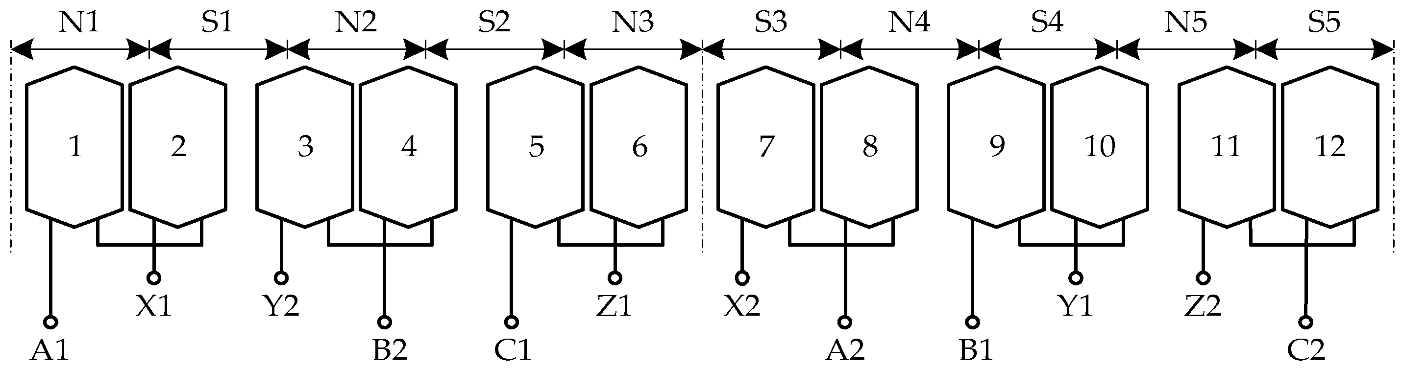
1. Introduction

The DRPMSM with weak thermal coupling and no electromagnetic coupling between phase winding is powered by two inverters. It can be applied in the fields of aerospace, national defense, and where needed to ensure the reliable operation of electric actuators [1]. In the PMSM drive system, the most common electrical fault is the inter-turn short circuit fault (ISCF) [2]. If the coil state is not detected and diagnosed during the initial stage of a fault, the fault may gradually deteriorate and spread, threatening the safety and reliability of the whole system, so on-line diagnosis of ISCFs is necessary. Domestic and overseas scholars have carried out research on many aspects of fault diagnosis in PMSM coils. In [3], the dual redundancy permanent magnet brushless DC motor (PMBDCM) is taken as the research object. Coil 5 is selected as the wavelet basis function to extract features of the current signal, and the neural network algorithm is used to diagnose the ISCF. In [4], a simple method of diagnosing the ISCF for three-phase windings with star connections is proposed. This method does not depend on the precise phasor calculation of voltage and current, but the analysis of voltage in the neutral point to realize the diagnosis. In [5], a dynamic modeling method for ISCF is introduced. For three-phase asymmetrical condition under fault, the positive and negative sequence components of current, flux linkage and voltage are acquired by symmetrical component method. In [6], a diagnostic method based on amplitudes of characteristic frequency components of load current as features. In [7], the extended dq matrix method is used to derive the formulas of dq-axis voltage of an 18-slot/6-pole PMSM before and after the fault occurs. Taking the current as fault signal, harmonic spectrum analysis is performed to determine whether the stator winding has an ISCF. In [8], the influence of different slot-pole match and the ISCF position of fault-tolerant PMSM on motor efficiency and short-circuit current are discussed. In [9], an adaptive fuzzy control system for PMBDCM is established. The power supply current waveform is used as a diagnostic signal to detect the ISCF. In [10], the fault diagnosis is performed by calculating the sum of phase voltages, and the fault phase and short-circuit turns are determined by discrete Fourier transform and short-time Fourier transform. In [11], a detailed derivation of the DRPMSM parameters is given and fault diagnosis is realized by analyzing the characteristics of the difference between straight-axis voltages.

In general, the research on ISCF diagnosis is concentrated on conventional PMSM, while there are few studies on the DRPMSM. When two sets of three-phase windings operate simultaneously, both of the current instructions come from a speed regulator. Although their current regulators are separated, due to the extremely fast adjustment of the current regulator, the currents of fault winding and healthy winding are almost equal when ISCF occurs, and as a consequence, many of the conventional diagnostic methods that use the fault characteristics of currents are not suitable for this type of DRPMSM. This paper analyzes the ISCF model of the DRPMSM from the two aspects of instantaneous reactive power and fundamental circuit theory combined with phasor analysis.

2. Introduction of the DRPMSM

The DRPMSM with weak thermal coupling and no electromagnetic coupling between phase winding is evolved from the traditional 12-slot/10-pole PMSM. Each phase consists of a positive and negative coil, so that there are no linkage between the armature reaction magnetic fields of each phase winding, but linkage of the slot leakage flux exists [12]. When a small tooth is added at the common slot, a passage is provided for the leakage flux, so the mutual inductance is almost zero, and the phase windings are electrically isolated. Insulating plates are placed on both sides of the small teeth, which can weaken the thermal coupling between different phase windings. The six phase windings of the stator can be divided into two sets of star connection windings with the same phase. Two sets are powered separately by two inverters, which improves the reliability of the system. A cross-sectional view of the DRPMSM is shown in Figure 1. The stator windings outspread diagram is shown in Figure 2.

Assuming that the mechanical angle of the small teeth is κ, the diagram of the fundamental EMF star graph and phase separation are shown in Figure 3. The main parameters of the DRPMSM are shown in

Table 1. The parameters of DRPMSM.

Parameter	Value
Rated power PN	3.5 kW
Rated speed nN	1200 rpm
Rated current IN	17.7 A
DC voltage Udc	200 V
Phase inductance L	2.19 mH
Phase resistance R	0.157 Ω
Permanent magnet flux linkage ψM	0.094 Wb
Coil number Nc	25
Pole pair p0	5
Half of small teeth κ	π/180 rad

.

3. The Mathematical Models of DRPMSM

3.1. Mathematical Model of Healthy Set

According to [11], there is no mutual inductance between the phase of the DRPMSM whether ISCF occurs or not, and the healthy set can be described by the circuit model shown in Figure 4.

The circuit matrix equation of the healthy set can be obtained from the Figure 4:

$$\left[\begin{array}{c}{u}_{\mathrm{A}1}\\ u_{\mathrm{B}1}\\ u_{\mathrm{C}1}\end{array}\right]=\left[\begin{array}{ccc}R& 0& 0\\ 0& R& 0\\ 0& 0& R\end{array}\right]\left[\begin{array}{c}{i}_{\mathrm{A}1}\\ i_{\mathrm{B}1}\\ i_{\mathrm{C}1}\end{array}\right]+\left[\begin{array}{ccc}L& 0& 0\\ 0& L& 0\\ 0& 0& L\end{array}\right]\frac{\mathrm{d}}{\mathrm{d}t}\left[\begin{array}{c}{i}_{\mathrm{A}1}\\ i_{\mathrm{B}1}\\ i_{\mathrm{C}1}\end{array}\right]+\left[\begin{array}{c}{e}_{\mathrm{A}1}\\ e_{\mathrm{B}1}\\ e_{\mathrm{C}1}\end{array}\right]+\left[\begin{array}{c}{u}_{01}\\ u_{01}\\ u_{01}\end{array}\right]$$

(1)

The valid value of the fundamental phase EMF by permanent magnet under normal conditions is as follows:

$$E=\frac{{\omega }_{\mathrm{e}}{k}_{q1}{k}_{y1}{N}_{\mathrm{c}}{\Phi }_{\mathrm{m}}}{\sqrt{2}}$$

(2)

where ${\omega }_{\mathrm{e}}$ (unit: rad/s) is the fundamental electrical angular velocity. $N_{\mathrm{c}}$ is the number of turns per coil. ${\Phi }_{\mathrm{m}}$ (unit: Wb) is the fundamental permanent magnetic flux of each pole. $k_{y1}$ is the fundamental pitch-shortening coefficient of coils. $k_{q1}$ is the fundamental distribution coefficient of coils.

When the mechanical angle of the small teeth $\kappa$ equals $\mathsf{\pi }/180$, $k_{y1}$ and $k_{q1}$ can be obtained by Equation (3):

$$k_{q1}=k_{y1}=\cos \left(\frac{\mathsf{\pi }}{12}+\frac{5\kappa }{2}\right)=\cos \left(\frac{7\mathsf{\pi }}{72}\right)$$

(3)

3.2. Mathematical Model of Faulty Set

Assuming that the phase C2 has an ISCF, which can be described by the circuit model shown in Figure 5a, where R_s is the resistance of the short-circuit turns, R_n is the resistance of the turns except for the short-circuit turns, L_s is the self-inductance of the short-circuit turns, M is the mutual inductance between short-circuit turns and the remaining normal turns, L_n is the self-inductance of the remaining normal turns, e_s is the EMF by permanent magnet of the short-circuit turns, e_n is the EMF of the remaining normal turns, R_f is the contact resistance where ISCF occurs, i_f is the current flowing through the contact resistance, i_s is the current flowing through the short-circuit turns, i_C2 is the phase current of C2. The reference direction of currents and EMF are marked in Figure 5a.

Assuming that the phase voltage is $u_{\mathrm{C}2}$, and applying Kirchhoff’s voltage law to Figure 5a:

$$\{\begin{array}{l}{R}_{\mathrm{s}}{i}_{\mathrm{s}}+L_{\mathrm{s}}\frac{\mathrm{d}{i}_{\mathrm{s}}}{\mathrm{d}t}+M\frac{\mathrm{d}{i}_{\mathrm{C}2}}{\mathrm{d}t}+e_{\mathrm{s}}+R_{\mathrm{f}}{i}_{\mathrm{f}}=0\\ -R_{\mathrm{f}}{i}_{\mathrm{f}}+L_{\mathrm{n}}\frac{\mathrm{d}{i}_{\mathrm{C}2}}{\mathrm{d}t}+M\frac{\mathrm{d}{i}_{\mathrm{s}}}{\mathrm{d}t}+i_{\mathrm{C}2}{R}_{\mathrm{n}}+e_{\mathrm{C}2}-e_{\mathrm{s}}=u_{\mathrm{C}2}\\ i_{\mathrm{s}}=i_{\mathrm{C}2}+i_{\mathrm{f}}\end{array}$$

(4)

Equation (5) can be obtained:

$$\{\begin{array}{l}{R}_{\mathrm{s}}{i}_{\mathrm{s}}+(L_{\mathrm{s}}+M)\frac{\mathrm{d}{i}_{\mathrm{s}}}{\mathrm{d}t}-M\frac{\mathrm{d}{i}_{\mathrm{f}}}{\mathrm{d}t}+e_{\mathrm{s}}+R_{\mathrm{f}}{i}_{\mathrm{f}}=0\\ -R_{\mathrm{f}}{i}_{\mathrm{f}}+(L_{\mathrm{n}}+M)\frac{\mathrm{d}{i}_{\mathrm{C}2}}{\mathrm{d}t}+M\frac{\mathrm{d}{i}_{\mathrm{f}}}{\mathrm{d}t}+i_{\mathrm{C}2}{R}_{\mathrm{n}}+e_{\mathrm{C}2}-e_{\mathrm{s}}=u_{\mathrm{C}2}\end{array}$$

(5)

According to Equation (5), the decoupling equivalent circuit of the circuit shown in Figure 5a can be obtained, as shown in Figure 5b. Using the Thevenin theorem, the circuit in Figure 5b can be simplified to that shown in Figure 5c. In Figure 5c, ΔR is the reduction of the equivalent resistance of the fault phase after ISCF occurs; ΔL is the reduction of the equivalent inductance; Δe is reduction of the equivalent induction EMF. The circuit with fundamental wave is the focused in the following sections.

If $\eta =N_{\mathrm{s}}/N_{\mathrm{C}}$, the effective value of the fundamental EMF by permanent magnet about the short-circuit turns shown in Figure 5b is given by:

$$E_{\mathrm{s}}=\frac{\sqrt{2}}{2}{\omega }_{\mathrm{e}}{k}_{y1}\eta N_{\mathrm{c}}{\Phi }_{\mathrm{m}}$$

(6)

After ISCF occurs, the equivalent impedance and open circuit voltage of the phase C2 are given by:

$$Z^{\prime }=\frac{[R_{\mathrm{s}}+\mathrm{j}{\omega }_{\mathrm{e}}(L_{\mathrm{s}}+M)](R_{\mathrm{f}}-\mathrm{j}{\omega }_{\mathrm{e}}M)}{(R_{\mathrm{s}}+R_{\mathrm{f}})+\mathrm{j}{\omega }_{\mathrm{e}}{L}_{\mathrm{s}}}+R_{\mathrm{cn}}+\mathrm{j}{\omega }_{\mathrm{e}}(L_{\mathrm{n}}+M)$$

(7)

$$\dot{E^{\prime }}={\dot{E}}_{\mathrm{C}2}-{\dot{E}}_{\mathrm{s}}+\frac{(R_{\mathrm{f}}-\mathrm{j}{\omega }_{\mathrm{e}}M)}{R_{\mathrm{s}}+R_{\mathrm{f}}+\mathrm{j}{\omega }_{\mathrm{e}}{L}_{\mathrm{s}}}{\dot{E}}_{\mathrm{s}}$$

(8)

Equations (9)–(11) can be derived through Equations (7) and (8):

$$\Delta R=R-\mathrm{Re}(Z^{\prime })=\frac{R_{\mathrm{s}}^3+R_{\mathrm{s}}^2{R}_{\mathrm{f}}+{\omega }_{\mathrm{e}}^2{R}_{\mathrm{s}}{L}_{\mathrm{s}}^2-R_{\mathrm{s}}{\omega }_{\mathrm{e}}^2{M}^2-R_{\mathrm{f}}{\omega }_{\mathrm{e}}^{2}M(L_{\mathrm{s}}+M)-{\omega }_{\mathrm{e}}^2{L}_{\mathrm{s}}(L_{\mathrm{s}}+M)R_{\mathrm{f}}}{{(R_{\mathrm{s}}+R_{\mathrm{f}})}^2+{\omega }_{\mathrm{e}}^2{L}_{\mathrm{s}}^2}$$

(9)

$$\Delta L=L-\frac{\mathrm{Im}(Z^{\prime })}{{\omega }_{\mathrm{e}}}=\frac{2M{R}_{\mathrm{s}}^2+L_{\mathrm{s}}{\omega }_{\mathrm{e}}^{2}M(L_{\mathrm{s}}+M)+L_{\mathrm{s}}{R}_{\mathrm{s}}(R_{\mathrm{s}}+2R_{\mathrm{f}})+2M{R}_{\mathrm{s}}{R}_{\mathrm{f}}+{\omega }_{\mathrm{e}}^2{L}_{\mathrm{s}}^3+{\omega }_{\mathrm{e}}^{2}M{L}_{\mathrm{s}}^2}{{(R_{\mathrm{s}}+R_{\mathrm{f}})}^2+{\omega }_{\mathrm{e}}^2{L}_{\mathrm{s}}^2}$$

(10)

$$\Delta \dot{E}={\dot{E}}_{\mathrm{C}2}-\dot{E^{\prime }}=\frac{(R_{\mathrm{s}}+\mathrm{j}{\omega }_{\mathrm{e}}M+\mathrm{j}{\omega }_{\mathrm{e}}{L}_{\mathrm{s}})}{R_{\mathrm{s}}+R_{\mathrm{f}}+\mathrm{j}{\omega }_{\mathrm{e}}{L}_{\mathrm{s}}}{\dot{E}}_{\mathrm{s}}$$

(11)

It can be seen from Equations (9) and (10) that $0<\Delta L<L/2$ is always true. The positive, negative and the magnitude of $\Delta R$ are affected by factors such as the number of short-circuit turns, operating frequency and contact resistance, but the relationship of $\Delta R<R_{\mathrm{s}}$ is always maintained.

In [11], the inductance parameters have been deduced in detail after ISCF occurs. Ignoring the small tooth angle $\kappa$ in the expression that has little influence on the inductance, the inductance of phase C2 can be given by:

$$\{\begin{array}{l}{L}_{\mathrm{s}}=\frac{11}{24}{\left(\frac{N_{\mathrm{s}}}{N_{\mathrm{c}}}\right)}^{2}L=\frac{11}{24}{\eta }^{2}L\\ M=\left[\frac{1}{2}\frac{N_{\mathrm{s}}}{N_{\mathrm{c}}}-\frac{11}{24}{\left(\frac{N_{\mathrm{s}}}{N_{\mathrm{c}}}\right)}^2\right]L=\left(\frac{1}{2}\eta -\frac{11}{24}{\eta }^2\right)L\\ L_{\mathrm{n}}=\left(1-\eta +\frac{11}{24}{\eta }^2\right)L\end{array}$$

(12)

Because the motor adopts the vector control mode of $i_d^{\ast }=0$, the phase of current fundamental wave is same with the EMF, and component of the negative sequence current caused by the ISCF is much smaller than that of the positive. When the mechanical angle of the small tooth $\kappa =\mathsf{\pi }/180$, from the phase relationship between the EMFs shown in Figure 3b, the positive sequence component of the phase fundamental wave current can be obtained as follows:

$$\{\begin{array}{l}{\dot{I}}_{\mathrm{A}}={\dot{I}}_{\mathrm{A}1}={\dot{I}}_{\mathrm{A}2}=I\angle \left(\frac{7}{72}\mathsf{\pi }\right)\\ {\dot{I}}_{\mathrm{B}}={\dot{I}}_{\mathrm{B}1}={\dot{I}}_{\mathrm{B}2}=I\angle \left(\frac{7}{72}\mathsf{\pi }-\frac{2}{3}\mathsf{\pi }\right)\\ {\dot{I}}_{\mathrm{C}}={\dot{I}}_{\mathrm{C}1}={\dot{I}}_{\mathrm{C}2}=I\angle \left(\frac{7}{72}\mathsf{\pi }+\frac{2}{3}\mathsf{\pi }\right)\end{array}$$

(13)

4. Calculation of the Reactive Power Difference Based on the Fundamental Wave Circuit

4.1. The Difference between Reactive Power by Traditional Power Theory

Regardless of the negative sequence component of the fundamental wave and harmonic currents in three phases, the complex power expression of the healthy phase C1 is given by:

$${\tilde{S}}_{\mathrm{Ch}}=(R{\dot{I}}_{\mathrm{C}}+{\dot{E}}_{\mathrm{C}}+\mathrm{j}{\omega }_{\mathrm{e}}L{\dot{I}}_{\mathrm{C}}){\dot{I}}_{\mathrm{C}}^{\ast }=R{I}_{\mathrm{C}}^2+{\dot{E}}_{\mathrm{C}}{\dot{I}}_{\mathrm{C}}^{\ast }+\mathrm{j}{\omega }_{\mathrm{e}}L{I}_{\mathrm{C}}^2$$

(14)

where ${\dot{I}}_{\mathrm{C}}^{\ast }$ is the conjugate complex of ${\dot{I}}_{\mathrm{C}}$.

The complex power expression of the faulty phase C2 is described by:

$$\begin{array}{cc}{\tilde{S}}_{\mathrm{Cf}}& =\left[\left(R-\Delta R\right){\dot{I}}_{\mathrm{C}}+j{\omega }_{\mathrm{e}}\left(L-\Delta L\right){\dot{I}}_{\mathrm{C}}+\left({\dot{E}}_{\mathrm{C}}-\Delta \dot{E}\right)\right]{\dot{I}}_{\mathrm{C}}^{\ast }\\ & =R{I}_{\mathrm{C}}^2+{\dot{E}}_{\mathrm{c}}{\dot{I}}_{\mathrm{C}}^{\ast }+\mathrm{j}{\omega }_{\mathrm{e}}L{I}_{\mathrm{C}}^2-(\Delta R{I}_{\mathrm{C}}^2+\Delta \dot{E}{\dot{I}}_{\mathrm{C}}^{\ast }+\mathrm{j}{\omega }_{\mathrm{e}}\Delta L{I}_{\mathrm{C}}^2)\end{array}$$

(15)

The difference between the reactive power of the two sets of windings are described as:

$$\Delta Q=\mathrm{Im}\left({\tilde{S}}_{\mathrm{Ch}}-{\tilde{S}}_{\mathrm{Cf}}\right)={\omega }_{\mathrm{e}}\Delta L{I}_{\mathrm{C}}^2+\Delta E{I}_{\mathrm{C}}\sin \xi$$

(16)

where $\xi$ is the advanced angle which $\Delta \dot{E}$ leads ${\dot{I}}_{\mathrm{C}}$.

It can be seen that after ISCF occurs, the reactive power of the healthy phase and the faulty phase are different. By calculating and comparing the difference of each phase’s reactive power, the faulty phase can be determined, and then the winding in which the ISCF occurs can be detected. However, according to the circuit theory, to get reactive power requires obtaining information on phase voltage, phase current, and phase relationship between them, the diagnostic cost will be greatly improved.

4.2. The Difference between Power by Akagi-Instantaneous-Power-Theory

In the early 1980s, Japanese scholar Akagi proposed a three-phase instantaneous power theory based on instantaneous values, namely the pq theory [13,14]. The core of the theory is to transform the three-phase instantaneous voltages and currents into the $\alpha \beta$ coordinate system, and the instantaneous reactive power $q$ is described as:

$$q=u_{\beta }{i}_{\alpha }-u_{\alpha }{i}_{\beta }$$

(17)

The instantaneous reactive power of the three-phase windings is the sum of the instantaneous reactive power of each phase. Therefore, the idea of “comparing the difference of each phase instantaneous reactive power to determine the faulty phase and the faulty set” can be converted into “comparing the difference between transient reactive power of two sets of windings to determine the faulty set directly.”

For the healthy set, the circuit matrix can be got by Equation (1) through Clark Transformation:

$$\left[\begin{array}{c}{u}_{\alpha 1}\\ u_{\beta 1}\\ 0\end{array}\right]=\left[\begin{array}{ccc}R& 0& 0\\ 0& R& 0\\ 0& 0& R\end{array}\right]\left[\begin{array}{c}{i}_{\alpha 1}\\ i_{\beta 1}\\ 0\end{array}\right]+\left[\begin{array}{ccc}L& 0& 0\\ 0& L& 0\\ 0& 0& L\end{array}\right]\frac{\mathrm{d}}{\mathrm{d}t}\left[\begin{array}{c}{i}_{\alpha 1}\\ i_{\beta 1}\\ 0\end{array}\right]+\frac{\mathrm{d}}{\mathrm{d}t}\left[\begin{array}{c}{e}_{\alpha 1}\\ e_{\beta 1}\\ 0\end{array}\right]+\sqrt{3}\left[\begin{array}{c}0\\ 0\\ u_{01}\end{array}\right]$$

(18)

The faulty set circuit matrix is described as:

$$\left[\begin{array}{c}{u}_{\mathrm{A}2}\\ u_{\mathrm{B}2}\\ u_{\mathrm{C}2}\end{array}\right]=\left[\begin{array}{ccc}R& 0& 0\\ 0& R& 0\\ 0& 0& R-\Delta R\end{array}\right]\left[\begin{array}{c}{i}_{\mathrm{A}2}\\ i_{\mathrm{B}2}\\ i_{\mathrm{C}2}\end{array}\right]+\left[\begin{array}{ccc}L& 0& 0\\ 0& L& 0\\ 0& 0& L-\Delta L\end{array}\right]\frac{\mathrm{d}}{\mathrm{d}t}\left[\begin{array}{c}{i}_{\mathrm{A}2}\\ i_{\mathrm{B}2}\\ i_{\mathrm{C}2}\end{array}\right]+\left[\begin{array}{c}{e}_{\mathrm{A}2}\\ e_{\mathrm{B}2}\\ e_{\mathrm{C}2}-\Delta e\end{array}\right]+\left[\begin{array}{c}{u}_{02}\\ u_{02}\\ u_{02}\end{array}\right]$$

(19)

And that in the $\alpha \beta$ coordinate system is given by:

$$\begin{array}{c}\left[\begin{array}{c}{u}_{\alpha 2}\\ u_{\beta 2}\\ 0\end{array}\right]=\left[\begin{array}{ccc}R& 0& 0\\ 0& R& 0\\ 0& 0& R\end{array}\right]\left[\begin{array}{c}{i}_{\alpha 2}\\ i_{\beta 2}\\ 0\end{array}\right]+\left[\begin{array}{ccc}L& 0& 0\\ 0& L& 0\\ 0& 0& L\end{array}\right]\frac{\mathrm{d}}{\mathrm{d}t}\left[\begin{array}{c}{i}_{\alpha 2}\\ i_{\beta 2}\\ 0\end{array}\right]+\frac{\mathrm{d}}{\mathrm{d}t}\left[\begin{array}{c}{e}_{\alpha 2}\\ e_{\beta 2}\\ 0\end{array}\right]+\\ \frac{2}{3}\left[\begin{array}{ccc}-\frac{1}{4}\Delta R& -\frac{\sqrt{3}}{4}\Delta R& \frac{1}{2\sqrt{2}}\Delta R\\ -\frac{\sqrt{3}}{4}\Delta R& -\frac{3}{4}\Delta R& \frac{\sqrt{3}}{2\sqrt{2}}\Delta R\\ \frac{1}{2\sqrt{2}}\Delta R& \frac{\sqrt{3}}{2\sqrt{2}}\Delta R& -\frac{1}{2}\Delta R\end{array}\right]\left[\begin{array}{c}{i}_{\alpha 2}\\ i_{\beta 2}\\ 0\end{array}\right]+\\ \frac{2}{3}\left[\begin{array}{ccc}-\frac{1}{4}\Delta L& -\frac{\sqrt{3}}{4}\Delta L& \frac{1}{2\sqrt{2}}\Delta L\\ -\frac{\sqrt{3}}{4}\Delta L& -\frac{3}{4}\Delta L& \frac{\sqrt{3}}{2\sqrt{2}}\Delta L\\ \frac{1}{2\sqrt{2}}\Delta L& \frac{\sqrt{3}}{2\sqrt{2}}\Delta L& -\frac{1}{2}\Delta L\end{array}\right]\frac{\mathrm{d}}{\mathrm{d}t}\left[\begin{array}{c}{i}_{\alpha 2}\\ i_{\beta 2}\\ 0\end{array}\right]+\sqrt{\frac{2}{3}}\left[\begin{array}{c}\frac{1}{2}\Delta e\\ \frac{\sqrt{3}}{2}\Delta e\\ -\frac{1}{\sqrt{2}}\Delta e\end{array}\right]+\sqrt{3}\left[\begin{array}{c}0\\ 0\\ u_{02}\end{array}\right]\end{array}$$

(20)

where $u_{\alpha }$, $u_{\beta }$, $i_{\alpha }$, $i_{\beta }$ are the voltages and currents in the $\alpha \beta$ coordinate system. The subscripts “1” and “2” respectively represent physical quantity associated with the healthy and the faulty set.

Equations (21) and (22) can be obtained by Equation (1):

$$u_{\alpha 1}=R{i}_{\alpha 1}+L\frac{\mathrm{d}}{\mathrm{d}t}{i}_{\alpha 1}+\frac{\mathrm{d}}{\mathrm{d}t}{e}_{\alpha 1}$$

(21)

$$u_{\beta 1}=R{i}_{\beta 1}+L\frac{\mathrm{d}}{\mathrm{d}t}{i}_{\beta 1}+\frac{\mathrm{d}}{\mathrm{d}t}{e}_{\beta 1}$$

(22)

According to Equations (17), (21) and (22), Equation (23) can be obtained:

$$q_1=\left(R{i}_{\beta 1}+L\frac{\mathrm{d}}{\mathrm{d}t}{i}_{\beta 1}+\frac{\mathrm{d}}{\mathrm{d}t}{e}_{\beta 1}\right)i_{\alpha 1}-\left(R{i}_{\alpha 1}+L\frac{\mathrm{d}}{\mathrm{d}t}{i}_{\alpha 1}+\frac{\mathrm{d}}{\mathrm{d}t}{e}_{\alpha 1}\right)i_{\beta 1}$$

(23)

Equations (24) and (25) can be obtained from Equation (20):

$$\begin{array}{c}{u}_{\alpha 2}=R{i}_{\alpha 2}+L\frac{\mathrm{d}}{\mathrm{d}t}{i}_{\alpha 2}+\frac{\mathrm{d}}{\mathrm{d}t}{e}_{\alpha 2}-\frac{2}{3}\left(\frac{1}{4}\Delta R{i}_{\alpha 2}+\frac{\sqrt{3}}{4}\Delta R{i}_{\beta 2}\right)-\\ \frac{2}{3}\left(\frac{1}{4}\Delta L\frac{\mathrm{d}}{\mathrm{d}t}{i}_{\alpha 2}+\frac{\sqrt{3}}{4}\Delta L\frac{\mathrm{d}}{\mathrm{d}t}{i}_{\beta 2}\right)+\sqrt{\frac{1}{6}}\Delta e\end{array}$$

(24)

$$\begin{array}{c}{u}_{\beta 2}=R{i}_{\beta 2}+L\frac{\mathrm{d}}{\mathrm{d}t}{i}_{\beta 2}+\frac{\mathrm{d}}{\mathrm{d}t}{e}_{\beta 2}-\frac{2}{3}\left(\frac{\sqrt{3}}{4}\Delta R{i}_{\alpha 2}+\frac{3}{4}\Delta R{i}_{\beta 2}\right)-\\ \frac{2}{3}\left(\frac{\sqrt{3}}{4}\Delta L\frac{\mathrm{d}}{\mathrm{d}t}{i}_{\alpha 2}+\frac{3}{4}\Delta L\frac{\mathrm{d}}{\mathrm{d}t}{i}_{\beta 2}\right)+\sqrt{\frac{1}{2}}\Delta e\end{array}$$

(25)

Substituting Equations (24), (25) into Equation (17), Equation (26) can be obtained:

$$\begin{array}{c}{q}_2=\left(R{i}_{\beta 2}+L\frac{\mathrm{d}}{\mathrm{d}t}{i}_{\beta 2}+\frac{\mathrm{d}}{\mathrm{d}t}{e}_{\beta 2}\right)i_{\alpha 2}-\left(R{i}_{\alpha 2}+L\frac{\mathrm{d}}{\mathrm{d}t}{i}_{\alpha 2}+\frac{\mathrm{d}}{\mathrm{d}t}{e}_{\alpha 2}\right)i_{\beta 2}-\\ \frac{2}{3}\left(\frac{\sqrt{3}}{4}\Delta R{i}_{\alpha 2}+\frac{3}{4}\Delta R{i}_{\beta 2}+\frac{\sqrt{3}}{4}\Delta L\frac{\mathrm{d}}{\mathrm{d}t}{i}_{\alpha 2}+\frac{3}{4}\Delta L\frac{\mathrm{d}}{\mathrm{d}t}{i}_{\beta 2}\right)i_{\alpha 2}+\sqrt{\frac{1}{2}}\Delta e{i}_{\alpha 2}+\\ \frac{2}{3}\left(\frac{1}{4}\Delta R{i}_{\alpha 2}+\frac{\sqrt{3}}{4}\Delta R{i}_{\beta 2}+\frac{1}{4}\Delta L\frac{\mathrm{d}}{\mathrm{d}t}{i}_{\alpha 2}+\frac{\sqrt{3}}{4}\Delta L\frac{\mathrm{d}}{\mathrm{d}t}{i}_{\beta 2}\right)i_{\beta 2}-\sqrt{\frac{1}{6}}\Delta e{i}_{\beta 2}\end{array}$$

(26)

Assuming that $i_{\alpha 1}=i_{\alpha 2}$, $i_{\beta 1}=i_{\beta 2}$, $e_{\alpha 1}=e_{\alpha 2}$, $e_{\beta 1}=e_{\beta 2}$, Equation (23) minus Equation (26), and Equation (27) can be obtained.

$$\begin{array}{c}\Delta q=\frac{\sqrt{3}}{6}\Delta R{i_{\alpha }}^2+\frac{1}{3}\Delta R{i}_{\alpha }{i}_{\beta }+\frac{\sqrt{3}}{6}\Delta L{i}_{\alpha }\frac{\mathrm{d}}{\mathrm{d}t}{i}_{\alpha }+\frac{1}{2}\Delta L{i}_{\alpha }\frac{\mathrm{d}}{\mathrm{d}t}{i}_{\beta }-\frac{\sqrt{3}}{6}\Delta R{i_{\beta }}^2-\\ \frac{1}{6}\Delta L{i}_{\beta }\frac{\mathrm{d}}{\mathrm{d}t}{i}_{\alpha }-\frac{\sqrt{3}}{6}\Delta L{i}_{\beta }\frac{\mathrm{d}}{\mathrm{d}t}{i}_{\beta }-\sqrt{\frac{1}{2}}\Delta e_{\mathrm{C}1}{i}_{\alpha }+\sqrt{\frac{1}{6}}\Delta e_{\mathrm{C}1}{i}_{\beta }\end{array}$$

(27)

Through the substitution of (28) into Equation (27):

$$\{\begin{array}{c}{i}_{\alpha }=\sqrt{\frac{3}{2}}{i}_{\mathrm{A}}\\ i_{\mathrm{A}}+i_{\mathrm{B}}+i_{\mathrm{C}}=0\\ i_{\beta }=\frac{1}{\sqrt{2}}{i}_{\mathrm{A}}+\sqrt{2}{i}_{\mathrm{B}}\end{array}$$

(28)

The difference of instantaneous reactive power between the healthy and faulty sets can be obtained:

$$\Delta q=\frac{\sqrt{3}}{3}(\Delta R{i}_{\mathrm{A}}^2+\Delta L{i}_{\mathrm{A}}\frac{\mathrm{d}}{\mathrm{d}t}{i}_{\mathrm{A}}+\Delta L{i}_{\mathrm{A}}\frac{\mathrm{d}}{\mathrm{d}t}{i}_{\mathrm{B}}-\Delta L{i}_{\mathrm{B}}\frac{\mathrm{d}}{\mathrm{d}t}{i}_{\mathrm{A}}-\Delta L{i}_{\mathrm{B}}\frac{\mathrm{d}}{\mathrm{d}t}{i}_{\mathrm{B}}-\Delta R{i}_{\mathrm{B}}^2+\Delta e{i}_{\mathrm{B}}-\Delta e{i}_{\mathrm{A}})$$

(29)

According to Equation (13), Equation (30) can be obtained:

$$\{\begin{array}{l}{\left(i_{\mathrm{A}}^2\right)}_{\mathrm{av}}={\left(i_{\mathrm{B}}^2\right)}_{\mathrm{av}}={\left(i_{\mathrm{C}}^2\right)}_{\mathrm{av}}=I_{\mathrm{C}}^2\\ {\left(i_{\mathrm{A}}\frac{\mathrm{d}}{\mathrm{dt}}{i}_{\mathrm{A}}\right)}_{\mathrm{av}}={\left(i_{\mathrm{B}}\frac{\mathrm{d}}{\mathrm{dt}}{i}_{\mathrm{B}}\right)}_{\mathrm{av}}={\left(i_{\mathrm{C}}\frac{\mathrm{d}}{\mathrm{dt}}{i}_{\mathrm{C}}\right)}_{\mathrm{av}}=0\\ {\left(i_{\mathrm{A}}\frac{\mathrm{d}}{\mathrm{dt}}{i}_{\mathrm{B}}\right)}_{\mathrm{av}}={\omega }_{\mathrm{e}}{I}_{\mathrm{C}}^2\sin \left(\frac{2}{3}\mathsf{\pi }\right)=\frac{\sqrt{3}}{2}{\omega }_{\mathrm{e}}{I}_{\mathrm{C}}^2\\ {\left(i_{\mathrm{B}}\frac{\mathrm{d}}{\mathrm{dt}}{i}_{\mathrm{A}}\right)}_{\mathrm{av}}={\omega }_{\mathrm{e}}{I}_{\mathrm{C}}^2\sin \left(-\frac{2}{3}\mathsf{\pi }\right)=-\frac{\sqrt{3}}{2}{\omega }_{\mathrm{e}}{I}_{\mathrm{C}}^2\\ {\left(\Delta e{i}_{\mathrm{B}}-\Delta e{i}_{\mathrm{A}}\right)}_{\mathrm{av}}=\sqrt{3}\Delta E{I}_{\mathrm{C}}\sin \xi \end{array}$$

(30)

Through the substitution of (30) into Equation (29), Equation (31) can be obtained:

$$\Delta q_{\mathrm{av}}={\omega }_{\mathrm{e}}\Delta L{I}_{\mathrm{C}}^2+\Delta E{I}_{\mathrm{C}}\sin \xi$$

(31)

Comparing with Equation (16) and Equation (31), it can be found that the average of differences between the instantaneous reactive power obtained by the Akagi instantaneous power theory is consistent with that by the traditional power theory.

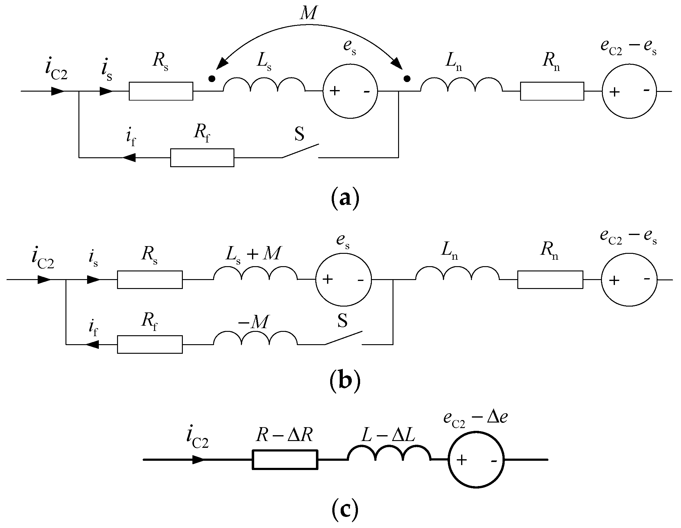
5. The Difference between Reactive Power after ISCF Occurs

If the contact resistance is not considered, substitute (12) into (11):

$$\Delta \dot{E}=\frac{{\dot{E}}_{\mathrm{s}}\left(\mathrm{j}{\omega }_{\mathrm{e}}M+\mathrm{j}{\omega }_{\mathrm{e}}{L}_{\mathrm{s}}+R_{\mathrm{s}}\right)}{R_{\mathrm{s}}+\mathrm{j}{\omega }_{\mathrm{e}}{L}_{\mathrm{s}}}=\frac{{\dot{E}}_{\mathrm{s}}\left(\mathrm{j}12{\omega }_{\mathrm{e}}L+12R\right)}{12R+\mathrm{j}11{\omega }_{\mathrm{e}}\eta L}=\dot{\sigma }{\dot{E}}_{\mathrm{s}}$$

(32)

$$\dot{\sigma }=\frac{\mathrm{j}12{\omega }_{\mathrm{e}}L+12R}{12R+\mathrm{j}11{\omega }_{\mathrm{e}}\eta L}=\sigma \angle {\varphi }_{\sigma }$$

(33)

where $\sigma$ is the amplitude of $\dot{\sigma }$, and ${\varphi }_{\sigma }$ is the phase angle of $\dot{\sigma }$.

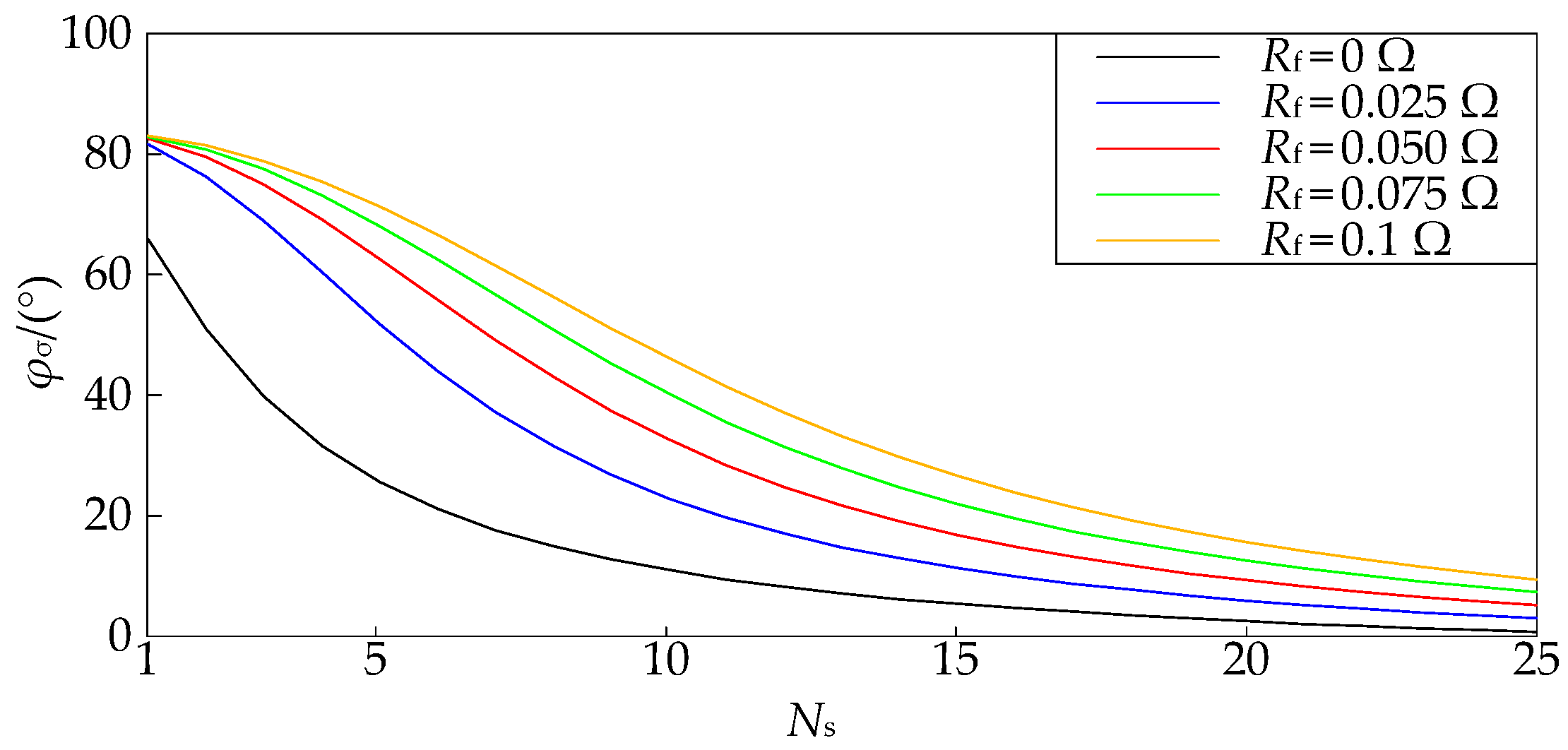
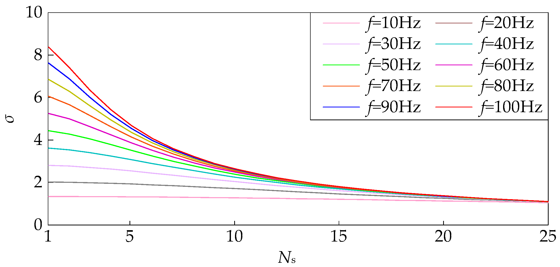
It can be seen from Equation (32) that the value of $\dot{\sigma }$ and ${\varphi }_{\sigma }$ depend on ${\omega }_{\mathrm{e}}$ and $\eta$. The parameters in Table 1 are introduced into Equation (32) to obtain the relationship curve which are shown in Figure 6 and Figure 7. It can be seen from the Figure 6 that $\sigma$ decreases with the increase of the number of short-circuit turns and increases with the increase of the operating frequency. When the number of short-circuit turns is large, the influence of the resistance in Equation (32) is negligible and $\sigma$ approaches a fixed value. ${\varphi }_{\sigma }$ decreases with the increase of number of short-circuit turns, eventually approaches 0, and increases first and then decreases as the operating frequency increases.

Considering the influence of contact resistance, if the motor operates at a rated frequency of 100 Hz, the curve of $\sigma$ and ${\varphi }_{\sigma }$ with the number of short-circuit turns and contact resistance are shown in Figure 8 and Figure 9, respectively.

When the number of short-circuit turns is small, since the denominator of the Equation (32) becomes larger after considering the contact resistance, $\sigma$ becomes smaller than that regardless of the contact resistance. With the number of short-circuit turns increases, the imaginary part of the denominator in the Equation (32) gradually plays a major role. So, the difference between the value of $\sigma$ and that regardless of the contact resistance is getting smaller and smaller, and they are almost equal when the number of short-circuit turns is large. Similarly, the introduction of contact resistance increases the real part of the denominator in Equation (32), thereby reducing the real part of Equation (32), leading to the final result that the value of ${\varphi }_{\sigma }$ increases. As can be seen from Figure 9, the greater the contact resistance is, the greater the degree of raising of ${\varphi }_{\sigma }$ is.

When the motor is running, according to Equation (31), the phase angle of $\Delta \dot{E}$ will be rotated counterclockwise by ${\varphi }_{\sigma }$ on the basis of ${\dot{E}}_{\mathrm{s}}$. The phase angle of ${\dot{E}}_{\mathrm{s}}$ coincides with the axis of the coil where the ISCF occurs, just like “12” or “-11” shown in Figure 10.

When the ISCF occurs at 12th tooth, the position of $\Delta \dot{E}$ relative to ${\dot{I}}_{\mathrm{C}}$ is shown in Figure 10. Obviously, $\xi$ is greater than 0. So, the difference of reactive power $\Delta q$ is a positive value.

When the ISCF occurs at 11th tooth regardless of the contact resistance $R_{\mathrm{f}}$, if the number of short-circuit turns is large, that is, $\eta \to 1$, ignoring the influence of the resistance $R$ in $\dot{\sigma }$, the phase angle of $\dot{\sigma }$ is close to 0 degree, and the phase of $\Delta \dot{E}$ is nearly same with that of ${\dot{E}}_{\mathrm{s}}$. The phase angle $\xi$ which $\Delta \dot{E}$ leads ${\dot{I}}_{\mathrm{C}}$ approaches −7π/72, and the value of ΔL is approximately L/2. Then, $\Delta q_{\mathrm{av}}$ can be described as:

$$\begin{array}{c}\Delta q_{\mathrm{av}}={\omega }_{\mathrm{e}}\Delta L{I}_{\mathrm{C}}^2+\frac{12}{11}\frac{\sqrt{2}}{2}{\omega }_{\mathrm{e}}{k}_{\mathrm{y}1}\eta N_C{\Phi }_{\mathrm{m}}{I}_{\mathrm{C}}\sin \left(-\frac{7}{72}\mathsf{\pi }\right)\\ ={\omega }_{\mathrm{e}}{I}_{\mathrm{C}}\left(\frac{L}{2}{I}_{\mathrm{C}}-\frac{6}{11}\sqrt{2}{N}_{\mathrm{C}}{\Phi }_{\mathrm{m}}\sin \frac{7}{72}\mathsf{\pi }\cos \frac{7}{72}\mathsf{\pi }\right)\\ ={\omega }_{\mathrm{e}}{I}_{\mathrm{C}}\left(\frac{L}{2}{I}_{\mathrm{C}}-\frac{3}{11}\sqrt{2}{N}_{\mathrm{C}}{\Phi }_{\mathrm{m}}\sin \frac{7}{36}\mathsf{\pi }\right)\end{array}$$

(34)

According to Equation (33) and the parameters in Table 1, when $I_{\mathrm{C}}$ is relatively small, $\Delta q_{\mathrm{av}}$ approaches 0. Actually, according to the above analysis, the existence of the contact resistance $R_{\mathrm{f}}$ will raise the phase angle ${\varphi }_{\sigma }$ of $\dot{\sigma }$(the contact resistance is relatively large at the beginning of the ISCF, and the degree of being raised of ${\varphi }_{\sigma }$ is large), which makes the angle $\xi$ that $\Delta \dot{E}$ leads ${\dot{I}}_{\mathrm{C}}$ greater than −7π/72, or even a positive value, thereby $\Delta q_{\mathrm{av}}$ will increase to be greater than 0. When I_C is relatively large, it is apparent that $\Delta q_{\mathrm{av}}$ is greater than 0.

If the number of short-circuit turns is small, i.e., $\eta \to 0$, the phase angle ${\varphi }_{\sigma }$ is large according to Figure 10. The angle $\xi$ that $\Delta \dot{E}$ leads ${\dot{I}}_{\mathrm{C}}$ is an acute angle which ensures $\Delta q_{\mathrm{av}}>0$.

By the analysis above, it is known that no matter which tooth the ISCF occurs at, there is a conclusion that $\Delta q_{\mathrm{av}}$ is greater than 0. When the motor is running, the faulty set is the one with relatively small instantaneous reactive power.

Actually, there are harmonic currents and correspondent negative sequence components in the model, and the motor parameters themselves are asymmetrical, so an appropriate threshold can be set in the diagnostic test to take those factors into consideration.

6. Simulation Analysis

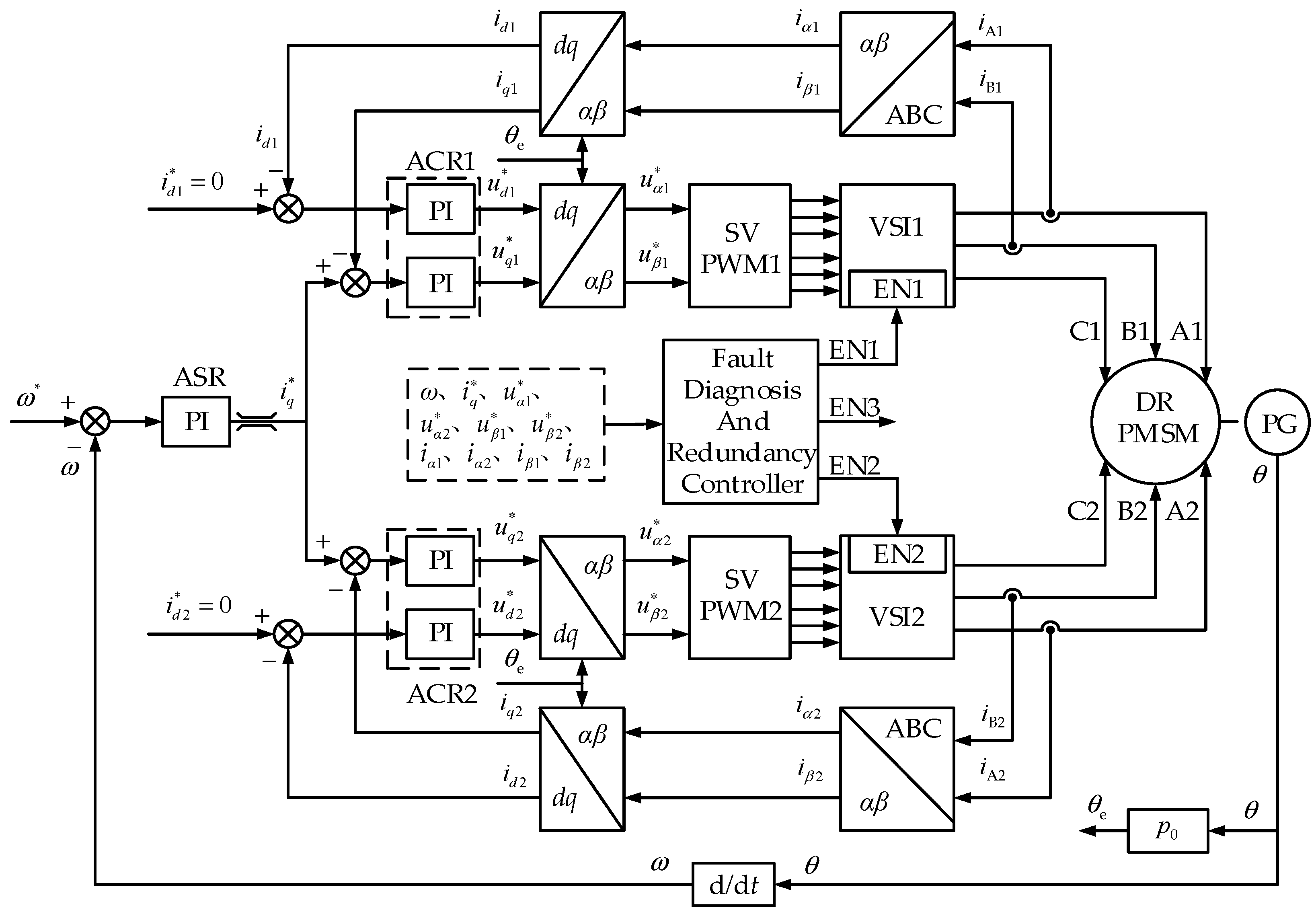
The simulation system block diagram of DRPMSM is shown in Figure 11.

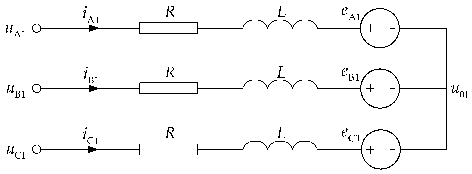
The voltages $u_{\alpha 1}^{\ast }$, $u_{\beta 1}^{\ast }$ and $u_{\alpha 2}^{\ast }$, $u_{\beta 2}^{\ast }$ represent the voltages $u_{\alpha 1}$, $u_{\beta 1}$ and $u_{\alpha 2}$, $u_{\beta 2}$ in reality. The formula for calculating the difference of instantaneous reactive power between the normal set and the fault set is given by:

$$\Delta q=\left[\left(u_{\beta 1}^{\ast }{i}_{\alpha 1}-u_{\alpha 1}^{\ast }{i}_{\beta 1}\right)-\left(u_{\beta 2}^{\ast }{i}_{\alpha 2}-u_{\alpha 2}^{\ast }{i}_{\beta 2}\right)\right]$$

(35)

The difference of the instantaneous reactive power $\Delta q$ between two sets can be obtained during system sampling period. If the average value of $\Delta q$ is got during the latest K periods and K is big, Equation (36) can be obtained:

$$\frac{1}{K}{\displaystyle \sum _{k=1}^K\Delta q}\left(k\right)\approx \Delta q_{\mathrm{av}}$$

(36)

The positive and negative of the average value can be treated as the diagnosis characteristic of the ISCF. The rated speed of the motor is 1200 r/min and the rated frequency is 100 Hz, which means the rated electrical period is 0.01 s. The value of K is the number of data collected within 0.01 s, which means the rated electrical period is set as the sampling calculation period. And the average value of these data is taken as the fault diagnosis characteristic to judge which set of winding is faulty in real time. When the average value is positive, the ISCF occurs in the second set of windings; conversely, the ISCF occurs in the first set.

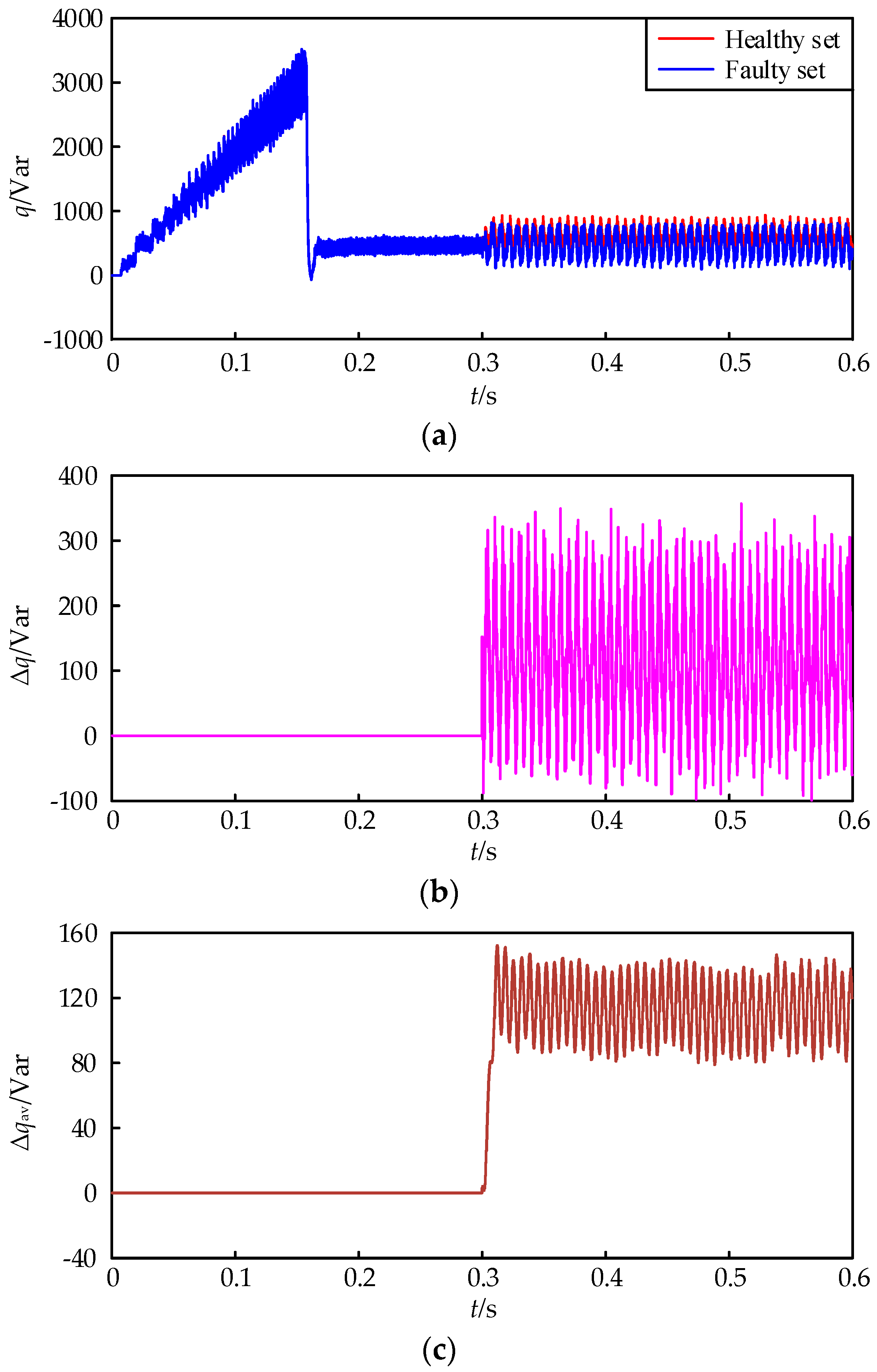
When the coils of 10 turns in the 12th tooth (phase C2) are shorted at 0.3 s (speed: 900 rpm, load torque: 20 N·m), the instantaneous reactive power curve are shown in Figure 12. According to Figure 12c, the average value is positive, so it is diagnosed that the ISCF occurs at the second set. The simulation system can be used to further analyze the factors affecting the difference of reactive power when ISCF occurs under the electrical operation condition.

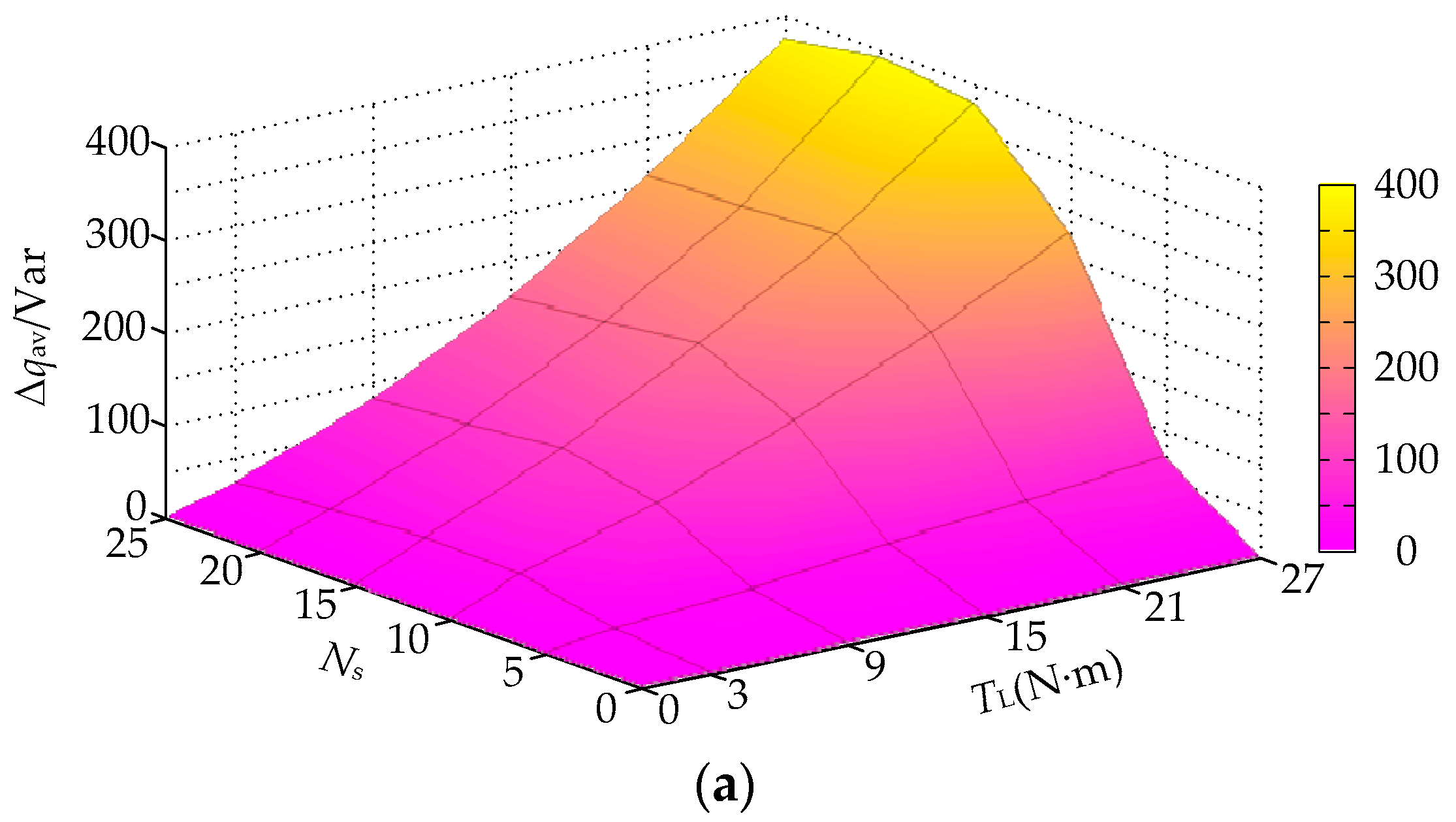
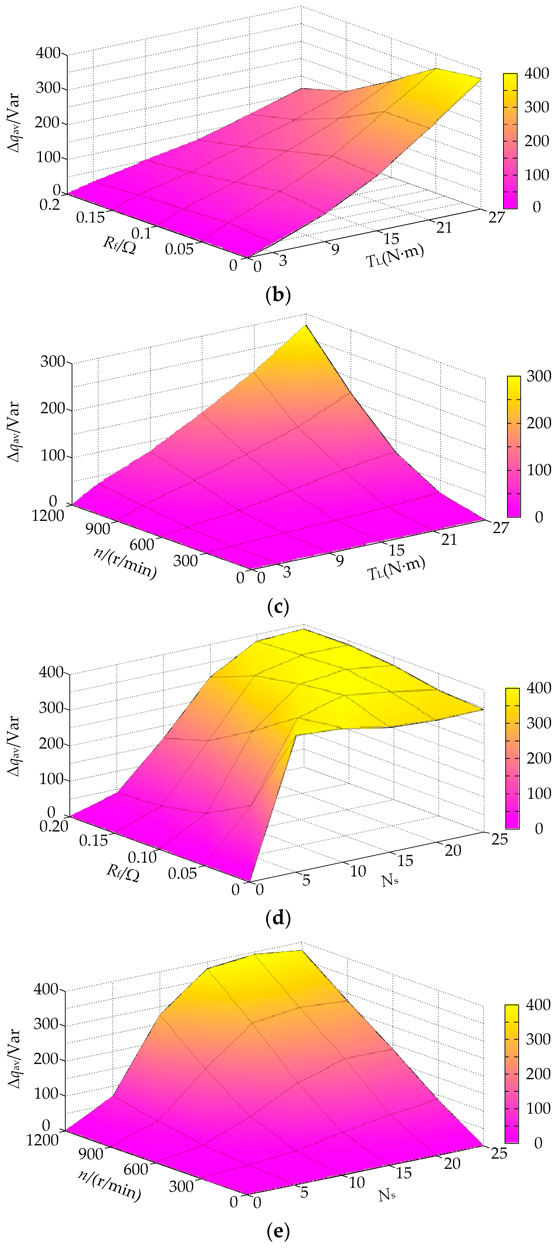
It can be seen from Equation (30) that the value of $\Delta q_{\mathrm{av}}$ is related to four factors such as the load, the number of short-circuit turns, contact resistance, and the speed. The values of the four variables are selected separately, and the obtained $\Delta q_{\mathrm{av}}$ are recorded. The results are shown in Figure 13 to observe the influence trend of different factors:

(1) The load

The larger the load is, the larger the value $I_{\mathrm{C}}$ is. As can be seen from Equation (30), both parts of $\Delta q_{\mathrm{av}}$ are positively correlated with the current $I_{\mathrm{C}}$, so the value of the fault characteristic gradually increases as the load increases. The simulation results reflecting these trends are shown in Figure 13a–c.

(2) Number of short circuit turns

It is known from Equation (30) that in the case other factors are constant, when the number of short-circuit turns is small, the contact resistance is bigger than the reactance of short-circuit turns. In addition, $\Delta L$ and $\Delta E$ are small, so the value of $\Delta q_{\mathrm{av}}$ is small. On the other hand, the current flowing through the contact resistance is small on condition that the small number of short-circuit turns, so the motor operates nearly at the normal state and $\Delta q_{\mathrm{av}}$ is small. As the number of short-circuit turns increases, $\Delta L$ and $\Delta E$ increase, and the value of short-circuit turns reactance gradually approaches that of the contact resistance. Through the Equation (31), as $\xi$ increases, $\Delta q_{\mathrm{av}}$ increases. When the number of short-circuit turns is big, its reactance approaches or even exceeds that of the contact resistance, which means the ISCF has been very serious. The value of $\Delta L$ approaches the maximum value of $L/2$, and $\Delta q_{\mathrm{av}}$ maintains a large value. However, since the value of $\xi$ gradually reduces during this process, the value of the fault characteristic may be reduced when the number of short-circuit turns is large. The entire process of change is like a curve “S” similar to the magnetization curve. The results are shown in Figure 13a,d,e.

(3) Contact resistance

When the contact resistance is larger than the reactance of short-circuit turns, the fault is light, and the conductors of coils are just beginning to contact, so $\Delta q_{\mathrm{av}}$ is small. As the fault gradually deteriorates, the adhesion between the coils becomes more and more serious, and the contact area becomes larger. As a result, the contact resistance becomes smaller, and the short-circuit becomes serious, so $\Delta q_{\mathrm{av}}$ maintains a large value. The results are shown in Figure 13b,d,f.

(4) The speed

When the load is constant and the speed is low, it is known from the Equations (10) and (11) that $\Delta L$ and $\Delta E$ are both small, and the value of $\xi$ is small, so the value of $\Delta q_{\mathrm{av}}$ is small. With the speed increasing, the values of $\Delta L$, $\Delta E$ and $\xi$ increase gradually, so $\Delta q_{\mathrm{av}}$ increases. The results are shown in Figure 13c,e,f.

The value of the fault characteristic is affected by the number of the load, short-circuit turns, the contact resistance and the speed from the above analysis. Those factors should be considered comprehensively when setting the threshold value of the fault characteristic. When the threshold set is larger, the fault of short-circuit can be diagnosed only if a certain load and a high speed. So, the rapidity of diagnosis is affected. If the threshold is smaller, the fault may be misjudged due to calculation error and external interference. The threshold can be set as a function related to the load (or $i_q$) and the speed, with different standards for the real-time operating conditions.

7. Experiments

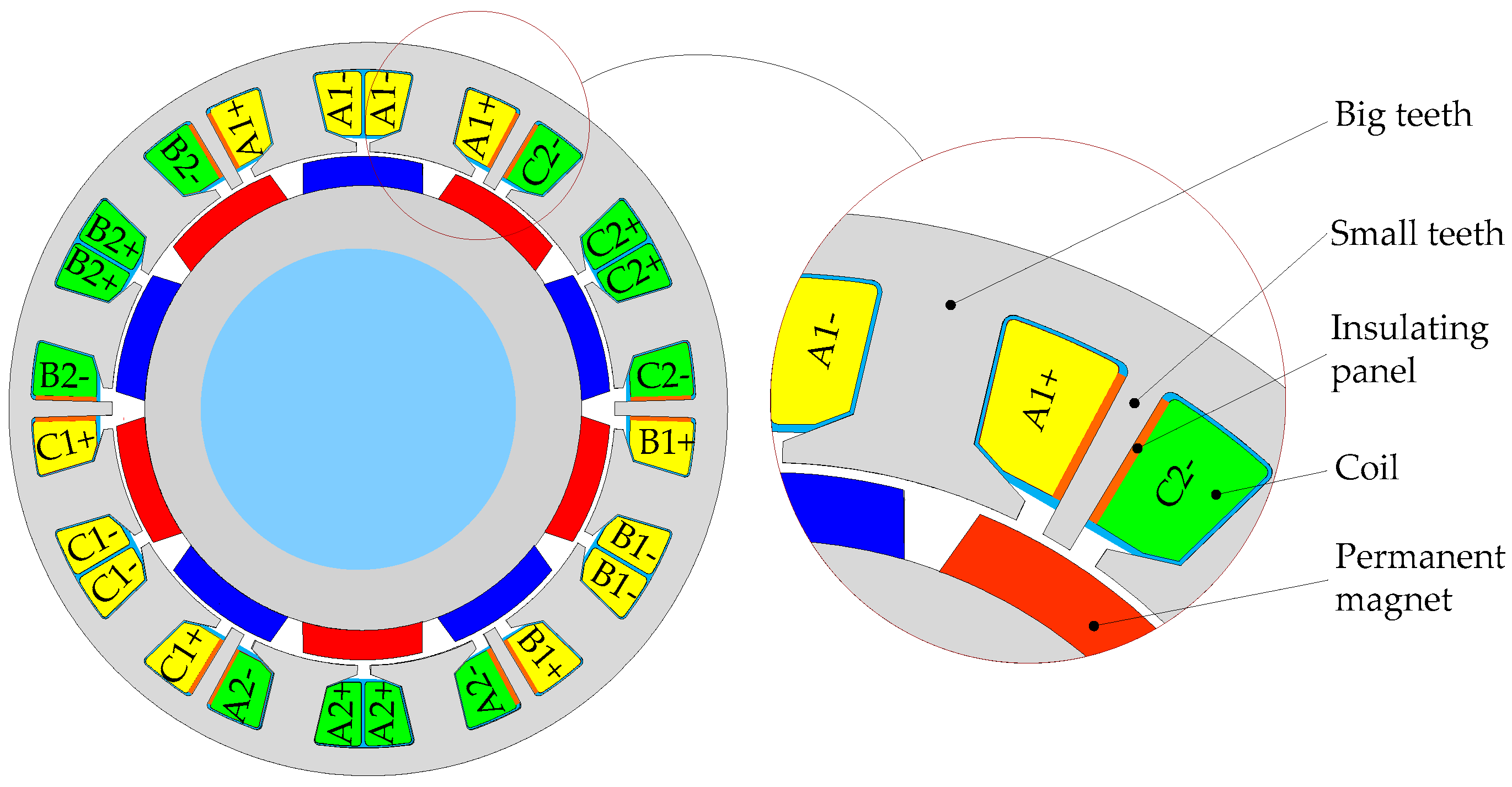
In order to verify the feasibility of the online diagnosis method after the ISCF proposed in this paper, the experimental system shown in Figure 14 was established. The experiment adopts the TMS320F2812DSP, and the load torque is provided by the magnetic powder brake. The speed in the experiment is 600 rpm, and a 10-turn coil around the 12th tooth is short-circuited. The contact resistance is 0.1 Ω, and the load torque is 16 N·m. In the experiment, DSP collects signals of $u_{\alpha 1}^{\ast },u_{\alpha 2}^{\ast },u_{\beta 1}^{\ast },u_{\beta 2}^{\ast },i_{\alpha 1},i_{\beta 1},i_{\alpha 2}$ and $i_{\beta 2}$ and transmit them to CAN, by which they are delivered to the host computer. Then the data can be exported and processed to establish the curves.

When the load torque is 16 N·m, the experimental results of the instantaneous reactive power are shown in Figure 15. In order to show the difference between the experimental results of the inter-turn short circuit fault and the normal condition, we add the $\Delta q_{\mathrm{av}}$ between two sets of windings under the normal operation in the Figure 15c. It is clear that $\Delta q_{\mathrm{av}}$ fluctuates around 0 when the motor is in normal operation, and $\Delta q_{\mathrm{av}}$ is obviously greater than 0 when the motor fails.

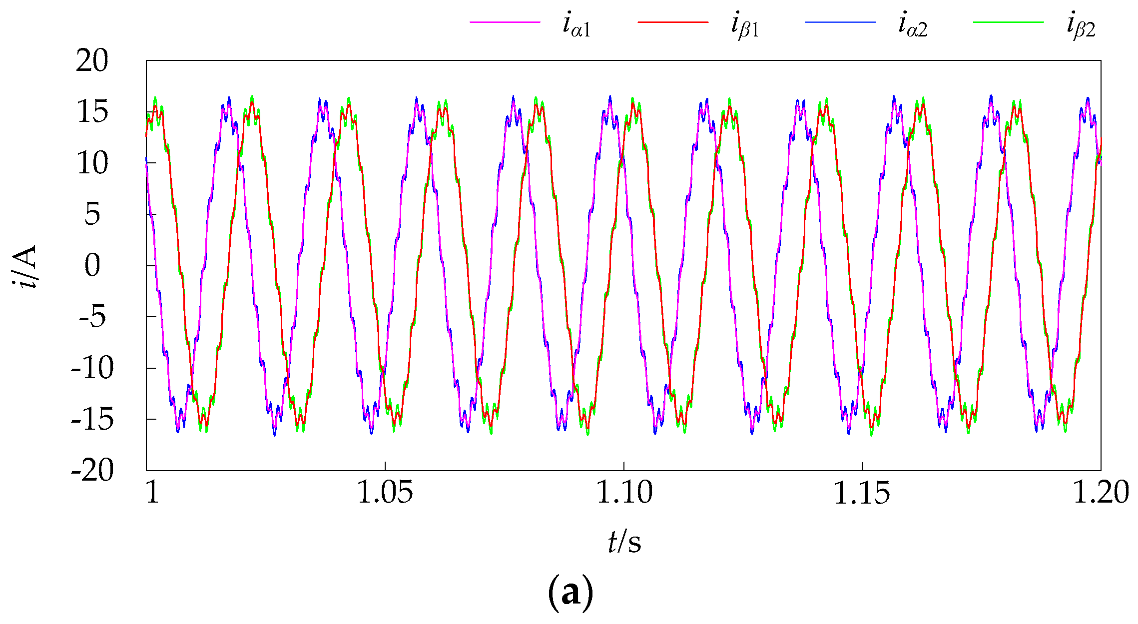
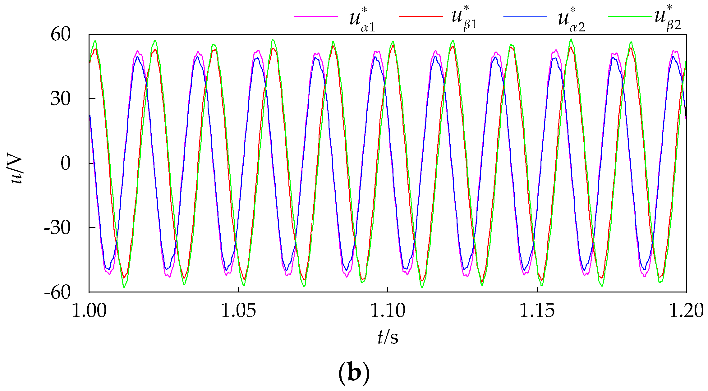
In order to observe clearly, the waveforms in 10 electrical cycles (1.00~1.20 s) in the experiment are selected. The experimental result of $i_{\alpha 1},i_{\alpha 2},i_{\beta 1},i_{\beta 2},u_{\alpha 1}^{\ast },u_{\alpha 2}^{\ast },u_{\beta 1}^{\ast },u_{\beta 2}^{\ast }$ are shown in Figure 16.

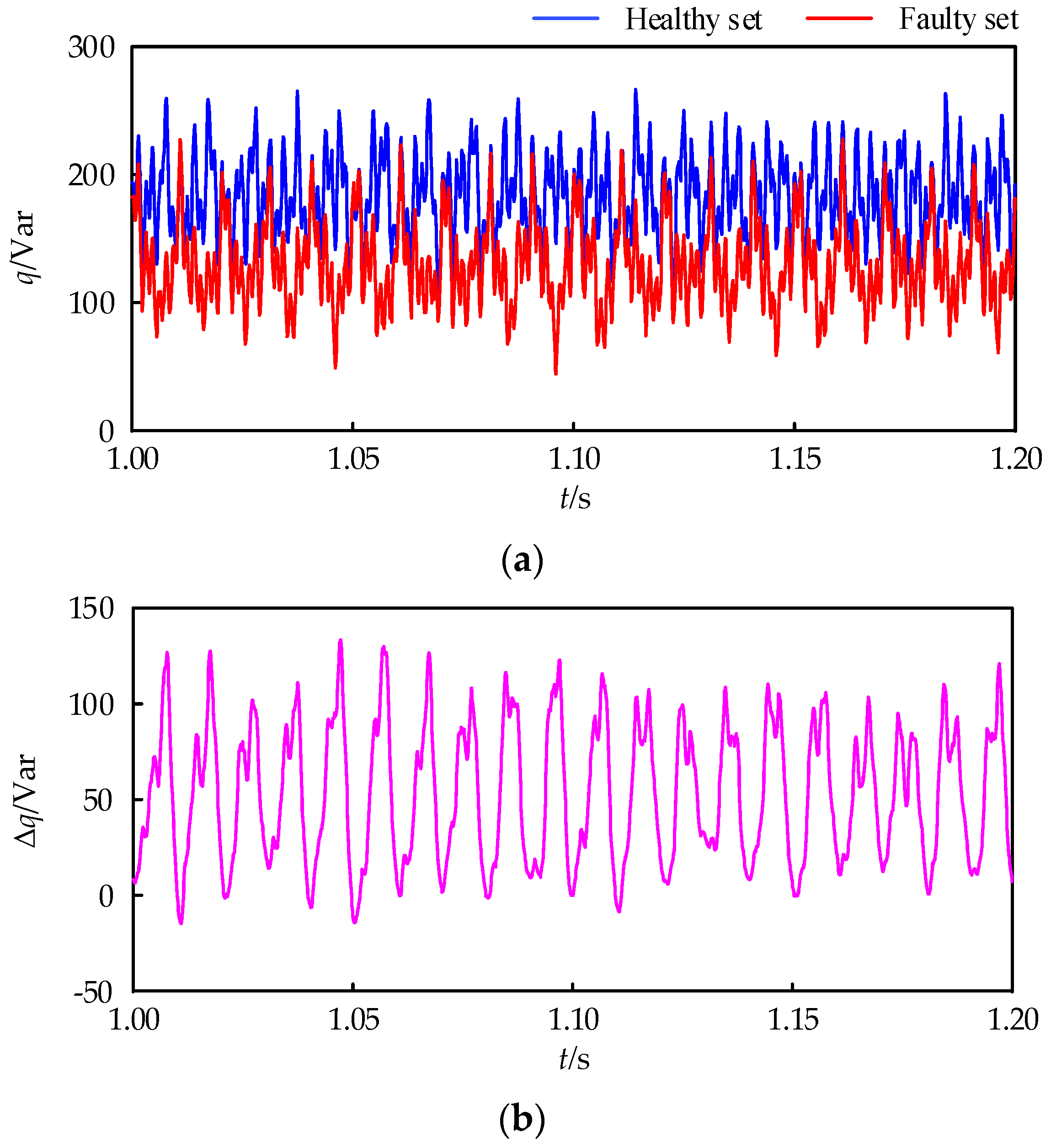
The waveforms of the instantaneous reactive power q and the difference of instantaneous reactive power $\Delta q$ between the two sets in 10 cycles are shown in Figure 17. 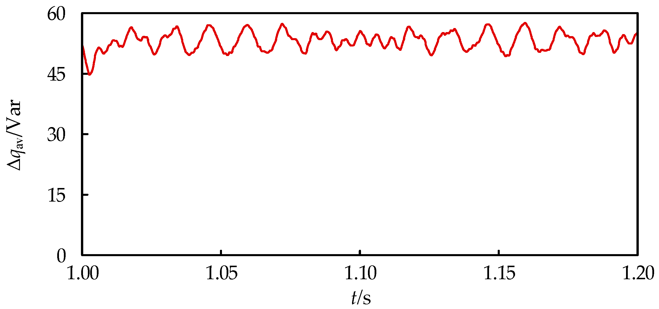In Figure 17b, the harmonic at the double frequency (100 Hz) is the main part, it is mainly caused by the negative sequence component of fundamental current and the third harmonic currents whose phase differences are $2\mathsf{\pi }/3$ electrical angle after inter-turn short circuit. The average value of $\Delta q_{\mathrm{av}}$ during this process is calculated with the period of 0.01 s shown in Figure 18. It can be concluded that when ISCF occurs, $\Delta q_{\mathrm{av}}$ is positive.

From the theoretical analysis, simulation and experimental verification of the above sections, it is feasible that the method of an online diagnosis for the ISCF of the DRPMSM based on instantaneous power theory proposed in this paper.

8. Conclusions

This paper focuses on a simplified circuit model of the DRPMSM after the ISCF occurs where the equivalent resistance, inductance and EMF are only considered without concerning harmonics. From the aspects of the traditional circuit theory and the Akagi instantaneous power theory, the reactive power of the healthy set and faulty set are calculated respectively based on the simplified circuit. And the results of the two theories are consistent with each other. The difference of the instantaneous reactive power between two sets is deduced in detail, and the characteristics of that are obtained from the phasor of the motor at different operating states. Therefore, a method based on the difference of instantaneous reactive power ($\Delta q$) between two sets of windings to realize on-line diagnosis of coil ISCF is proposed. Qualitative analysis and simulation show the trends of $\Delta q$ affected by several factors such as the number of short circuit turns, motor speed, contact resistance and load torque. And by the theoretical analysis, simulation and experimental verification, it is feasible that an online diagnosis method for the ISCF of DRPMSM based on instantaneous power theory in this paper.