Monetary Policy Effects on Energy Sector Bubbles

Abstract

We investigate the effects of monetary policy shocks, including unconventional policy measures, on the bubbles of the energy sector, for the case of the United States. We estimate a time-varying Bayesian VAR model that allows for quantifying the impact of monetary policy shocks on asset prices and bubbles. The energy sector is measured through the S&P Energy Index, while bubbles are measured through the difference between asset prices and the corresponding dividends for the energy sector. We find significant differences in the impact of monetary policy shocks for the aggregate economy and for the energy sector. The findings seem sensitive to the interest rate use, i.e., whether one uses the shadow interest rate or the long-term interest rate.

1. Introduction

The energy sector has proven to be very dynamic in the last decade. On one hand, there have been large swings in energy (especially oil) prices which are hard to be reconciled with the fundamentals, see [1]. In addition to this, we have witnessed the rapid emergence of new technologies that have pushed energy prices further lower, while fueling a boom in the energy sector that propelled the United States among the first oil producers in the world. On the other hand, the general picture is filled by a post-crisis macroeconomic environment where there is a reliance of key central banks in developed countries on quantitative easing, as a measure to counter the effects of the Great Recession. This has without doubt limited the ability to understand the dynamics of energy prices, as well as the dynamics the energy sector as a whole.

While there has been some research that deals with the effects of monetary policy at zero lower bound on energy (or oil) prices, the behavior of energy stocks has been far less discussed.

In this paper, we aim to answer two research questions. Firstly, we are interested in studying what are the effects of monetary policy on the energy sector. In addition to this, we scrutinize the manner in which bubbles in energy sector stocks responded to the dynamics of monetary policy, especially during the zero lower bound period.

As already mentioned, there has been some work dealing with the effects of conventional or unconventional monetary policy on energy prices, especially oil. Ref. [2] discussed the effects of US monetary policy on commodity prices. Their main finding is that expansionary US monetary policy shocks led to increases in global commodity prices.

Along the same line, but with a deeper focus, Ref. [3] study the effects of US monetary policy on sectoral commodity prices employing a vast array of assets, ranging from food and beverage prices to energy commodities. Using a Structural Vector Autoregression (SVAR) model setup, the authors notice that a contraction of monetary policy translates into a swift escalation of the broad commodity price index. Even with more relevance to the present paper, Ref. [3] also report that a positive interest rate shock determines a steady reduction in energy and metals prices. Similar results are obtained in the large-scale investigation of [4] which is dedicated to the interaction between oil prices and global macroeconomic factors. By means of a global factor-augmented error correction model, the study finds that positive innovations in global interest rates are associated with declines in global oil prices.

On a different note, Ref. [5] seeks to determine whether US monetary policy responds to changes in energy prices. Relying on a multi-sector version of the Smets-Wouters (SW) model estimated in a Bayesian approach, Kara (2017) argues that despite the mainstream view that stipulates a lack of reaction, the results point to the fact that the US central bank considers energy prices in the policy rule.

In another very recent contribution, Ref. [6] study the connections between energy prices and innovations in monetary policy deriving from the Federal Open Market Committee’s announcements. The authors find abnormal behavior in terms of price dynamics surrounding monetary policy announcements. Moreover, the abnormal behavior tends to be proportional to the expected modifications of policy rate. In addition to this, the authors argue in favor of pre-announcement effects via volatility channels.

Ref. [7] analyzed the effects of monetary policy in the United States on oil prices, using high frequency data. Quite significantly, the author looked at both conventional and unconventional monetary policy measures, relying on an event study framework. He employed three types of monetary policy surprises: surprise changes in federal funds rate, surprise changes in the future path of monetary policy and surprise changes in the future large-scale purchases. The study reported significant effects of monetary policy surprises. For example, a 1% rise in the interest rate led to a decrease of 3% in oil prices. Unconventional monetary policy measures had similar effects, though a bit larger.

There is also some consistent literature on the speculative elements in energy prices, especially for oil prices. For example, Ref. [8] found a significant explanatory power of the financial component for oil prices after 2000. At the same time, according to the above-mentioned study, the swing in oil prices during the 2007–2008 financial crisis was mainly due to macro-financial factors. Focusing rather on extreme events, Ref. [9] studied extreme oil prices increases and reported that even though acute, these price movements could be explained based on fundamentals.

Although not directly related to our work, it is worth mentioning other investigations on the impact of monetary policy on oil prices (or commodity prices). Ref. [10] considered the assumption that the US monetary policy could be considered a driver of oil prices. By implementing a cointegrated vector autoregression procedure, the authors observed that monetary shocks led to adjustments in both oil and industrial prices. The study also concluded that oil prices adjusted faster to monetary shocks than industrial prices.

More recently, Ref. [11] focus on the potential cross-correlations between US monetary policy, the US dollar index and the crude oil market (WTI). Using a multifractal detrended cross-correlation analysis (MF-DCCA) approach, the authors argue in favor of multifractal features for the cross-correlation between the variables. Moreover, Ref. [11] report that the monetary policy actions determine clear effects on the cross-correlated dynamics of the other series.

Ref. [12] focused on a related topic, namely the way the US monetary policy responses should vary in accordance to oil price fluctuations. In a two-block dynamic stochastic general equilibrium model (DSGE) setup, the authors documented on the way in which the monetary policy is affected by shocks that alter oil prices.

In this paper, we contribute to the debate regarding the design and effects of monetary policy in the aftermath of the crisis, by focusing on one of the most dynamic sectors, namely the energy sector. On one hand, the energy sector in the United States has passed through a recent boom due to current technological advances. On the other hand, commodity prices have been very volatile in the last decade. Thus, the focus of the research on the energy sector is fully justified.

In contrast to previous work, we focus on the behavior of the firms in the energy sector. Clearly, there is a positive link between the dynamics of market evaluations of energy stocks and the fluctuations of current and future commodity prices. Energy companies are the main actors in the energy sector, and investors’ perceptions on the future dynamics of commodity prices will be reflected in the market values of the energy companies.

There are also additional reasons for which studying the behavior of energy sector stocks is of interest. Recent research by [13,14] or [15], to cite only a few papers, has outlined the impact of monetary policy shocks on stock market bubbles.

Despite the lack of studies dealing directly with the connection between monetary policy and energy market bubbles, there is a block of literature dedicated to the investigation of bubbles endemic to energy markets. Without having the purpose of offering an exhaustive review, we mention the contribution of [16] that aims to determine the potential existence of instances of explosive behavior in crude oil, heating oil, and natural gas indices, as well as in WTI, Brent, natural gas, jet fuel and heating oil spot prices. In a first step, the authors notice explosive patterns for all energy series and then manage to isolate bubble episodes for four out of five spot prices series. Comparable results are obtained in a similar methodological approach by [17] for the case of spot and futures prices for oil, gasoline, and coal.

It is, therefore, relevant for policy makers, investors, and academics to learn how the energy sector and the measured bubbles in this sector, have reacted to the changing monetary policy conditions, especially in the aftermath of the financial crisis. This can help in understanding the sustainability of the recent booms in green energy, see [18] for a study, or the prospects of continuing the accelerated development in the shale production in the US and other countries, as reported by [19].

This paper brings several contributions. Firstly, we propose one of the first studies that identifies not only the effects of monetary policy shocks on the energy stocks, but also the responses of bubbles in the energy sector to such shocks. Secondly, we contribute to the recent literature on bubbles by focusing on a specific sector, in contrast to most of the research that considered the aggregate behavior of an economy. We also contribute to the ongoing research effort that studies the sustainability of the recent booms in the various activities of the energy industry.

2. A Bayesian Time-Varying VAR Approach

This section briefly details the time-varying Bayesian VAR designed to isolate the influence of monetary policy shocks on bubbles, which incorporates the specifications of [20]. From a technical perspective, our time-varying Bayesian autoregressive model takes the following form:

$$x_t=A_{0,t}+A_{1,t}{x}_{t-1}+\dots +A_{p,t}{x}_{t-p}+u_t$$

(1)

$A_{0,t}$ denotes a vector of time-varying intercepts and at the same time the $A_{i,t}$ matrices carry the time-varying coefficients. We consider $u_t$ to be a white noise Gaussian process with zero mean and ${\mathsf{\Sigma }}_t$ as covariance matrix.

Our approach treats innovations as linear transformations of the structural shocks such that: $u_t=S_t{ϵ}_t$. In addition to this, we note that $E\left\{{ϵ}_t{ϵ}_t^{\prime }\right\}=I$ and $E\left\{{ϵ}_t{ϵ}_{t-k}^{\prime }\right\}=0$. Moreover, we also assume that: $S_t{S}_t^{\prime }={\mathsf{\Sigma }}_t$.

In the spirit of [14] we assimilate the identification procedure introduced by [21]. The following ordering of the variables is used: $y_t,p_t,d_t,p_t^e,i_t,q_t$, with $y_t$ log of GDP, $p_t$ log of the GDP deflator, $d_t$ the log of real dividends, $p_t^e$, the log of World Bank commodity prices index, $i_t$ the interest rate, and $q_t$ the log of the stock market index (or the corresponding index for the energy sector).

In this specification based on the Choleski ordering of the variables, the monetary policy shocks are assumed not to affect contemporaneously the Gross Domestic Product, the inflation or the dividends, while, furthermore, the central bank does not respond contemporaneously to innovations in real stock prices.

We do not perform changes in the ordering of the VAR model, since the literature, see [21], or [14], explains that we should expect the central bank not to react contemporaneously to stock market changes, while the stock market responds to interest rate changes. Changing the ordering by placing the interest rate as last variable would make the stock market not react to interest rate changes.

3. Data

Our data set follows the specifications of [14] and focuses on a sample ranging from 1992 Q1 to 2016 Q4. It contains seven variables specific to the US. The data can be divided into two main categories: macroeconomic and financial. The first set comprises of: GDP, GDP deflator, the interest rate, and a non-energy commodity price index, data that have as source the OECD, FRED or the World Bank. Our second set focuses on the returns of the S&P 500 Energy Sector Index (GICS Level 1) and its associated dividends. All financial data have been obtained from Bloomberg.

Moreover, our methodology also relies on the use of shadow rates formulated in the study by [22] for the case of the Federal Reserve. This is done to take into account the fact that the nominal interest rate has hit the zero lower bound and thus, for a few years, has ceased to be a relevant measure of the monetary policy stance. As a robustness exercise, we also re-estimate the models using the long-term interest rate corresponding to the 10-year US bonds.

The descriptive statistics related to the data are presented below. We treat all data in log difference form, except for the two interest rates, to long term interest rate and the shadow rate. The basic statistics are shown in

Table 1. Descriptive statistics.

Country	Mean	Std. Deviation	Max	Min	Jarque-Bera
GDP	0.14	0.62	1.35	−4.80	24.65
GDP deflator	0.47	0.21	1.11	−0.16	4.80
Stock Market	1.20	11.80	−31.83	6.23	280.43
Stock Market Energy	1.43	9.18	18.4	−29.37	4.80
Real Dividends	0.84	2.01	4.60	6.87	81.33
Real Dividends for Energy	0.94	23.52	105.99	−106.13	206.6
World Bank Price index	0.53	5.85	13.67	−36.39	4.80
Shadow rate	2.35	6.52	2.77	2.77	8.03
Long-term interest rate	4.45	1.67	7.83	1.56	4.49

.

4. Results

4.1. Testing for Causality

The time-varying BVAR used in the following section, although able to detect the impact of different shocks, including that of monetary policy shocks, cannot decide whether there is a causality mechanism between monetary policy changes and the formation of bubbles. Although some theoretical mechanisms were discussed in [13], the empirical evidence is limited to the subsequent study by [14].

We include below the results for Granger causality tests between the interest rate used in the estimation of the BVAR model, the shadow interest rate, as well as the alternative measure, the long term interest rate (10 years bonds yield), see

Table 2. Granger Causality tests: shadow interest rate.

Country	1 Lag	2 Lags	3 Lags	4 Lags	8 Lags
Stock Market	0.02	0.42	1.14	2.15 *	2.22 **
Stock Market Energy	0.96	1.13	1.71	2.53 **	1.56
Real Dividends	1.59	1.15	1.04	1.45	1.89 *
Real Dividends for Energy	0.07	0.39	0.42	0.33	0.42

Note: * denotes statistical significance of the F statistic at the 0.10 level; ** at the 0.05 level; and *** at 0.01 level.

and

Table 3. Granger Causality tests: long-term interest rate.

Country	1 Lag	2 Lags	3 Lags	4 Lags	8 Lags
Stock Market	0.02	1.05	0.55	0.51	1.92 *
Stock Market Energy	0.20	0.28	0.60	1.54	0.91
Real Dividends	0.18	0.81	0.72	0.86	3.25 ***
Real Dividends for Energy	0.06	0.76	0.42	0.32	0.46

Note: * denotes statistical significance of the F statistic at the 0.10 level; ** at the 0.05 level; and *** at 0.01 level.

.

The results above indicate some traces of causality from the two interest rates used, to the stock market, especially at higher lags. This is rather in line with the large literature showing that movements in the exchange rates do matter for stock market fluctuations. This assertion is also verified for the Energy Index, though less for the case of long-term interest rates (which might give a different signal to the markets in the end). The discussion in literature on the effects of monetary policy shocks on dividends is less developed, since dividends are largely the results of economic activity. In our case, there are some instances at larger lags (up to 2 years) of causality from monetary policy to dividends, but not for the energy sector (in which there is also a large volatility for dividends).

4.2. Estimation

We estimate a Bayesian time-varying VAR model for the sample between 1992 Q1 and 2016 Q4. The settings are similar to those in [14]. To estimate the model, we use the Gibbs sampling algorithm put forward by [23]. As for the prior distributions, it is presumed that the covariance matrices $\mathsf{\Omega },\mathsf{\Xi },\mathsf{\Psi }$ and the initial states ${\theta }_0,{\varphi }_0,log{\sigma }_0$ are independent, and that the prior distributions for the initial states are set as normal distributions, while for ${\mathsf{\Omega }}^{-1},{\mathsf{\Xi }}^{-1},{\mathsf{\Psi }}^{-1}$ we use Wishart distributions. For the normal distributions, the prior means and variances are derived from an estimated time-invariant VAR on a sub-sample. We use 22,000 draws for the estimation of the model, but discard the first 20,000 to keep 2000 draws, following basically the approach in [14].

We perform two estimations: one on the extended original data sample provided by [14], and an alternative estimation that focuses on the energy sector, i.e., we use the S&P data for the energy sector, as well as the corresponding dividends. It must be noted that our data differ from the setup in [14] also by the use of the shadow interest rate.

4.3. The Impact of Monetary Policy Shocks on the Energy Sector

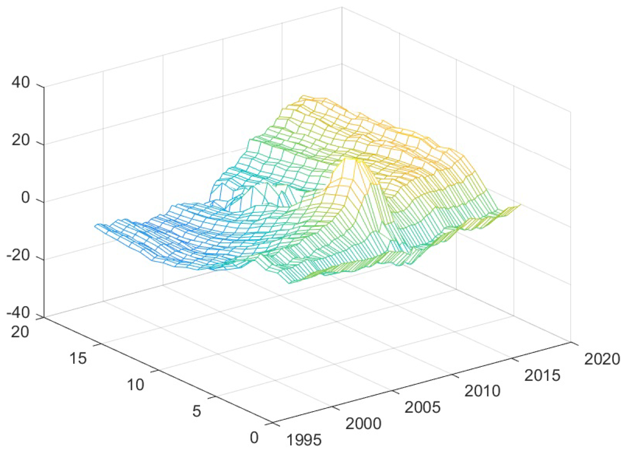
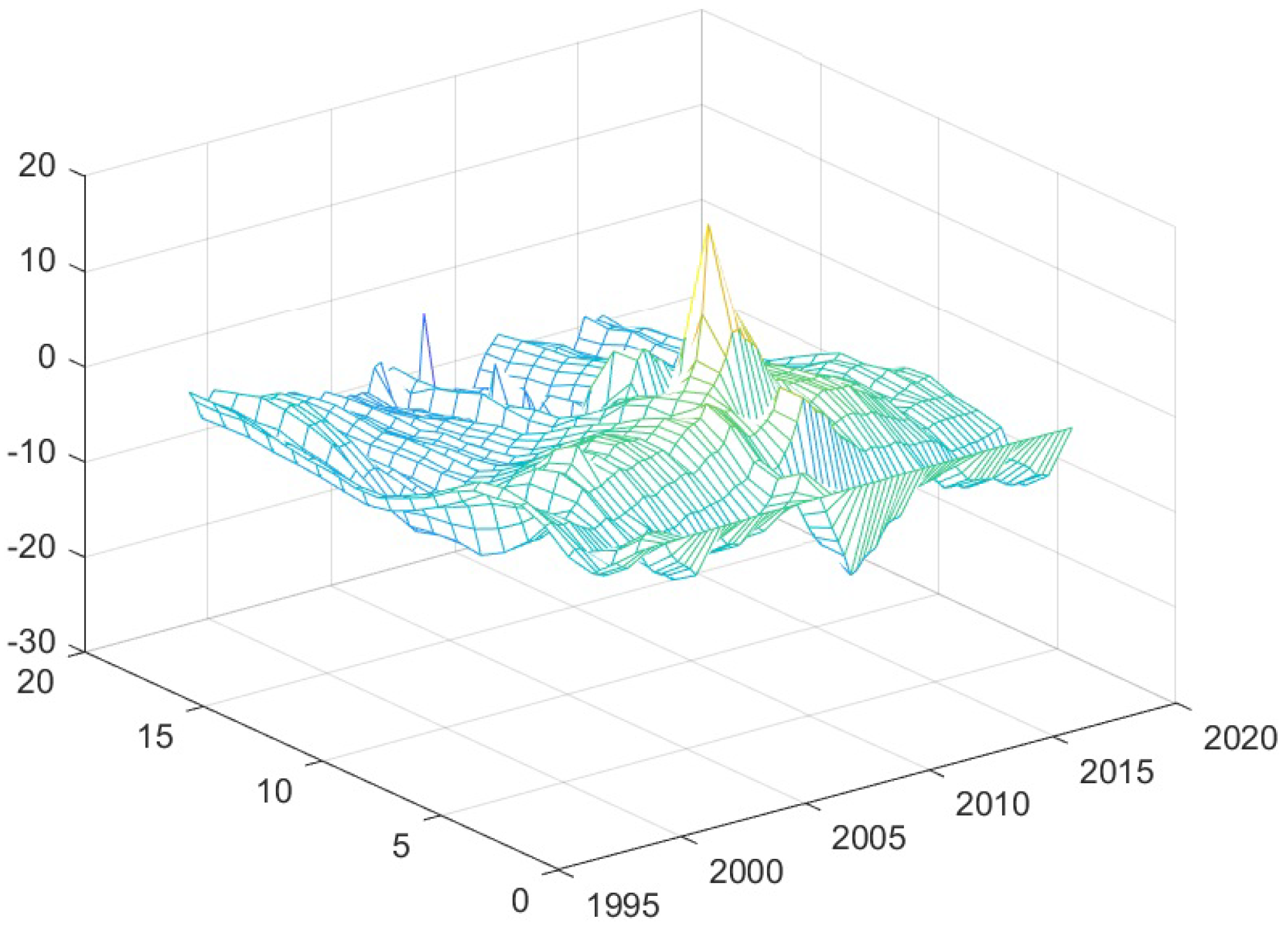
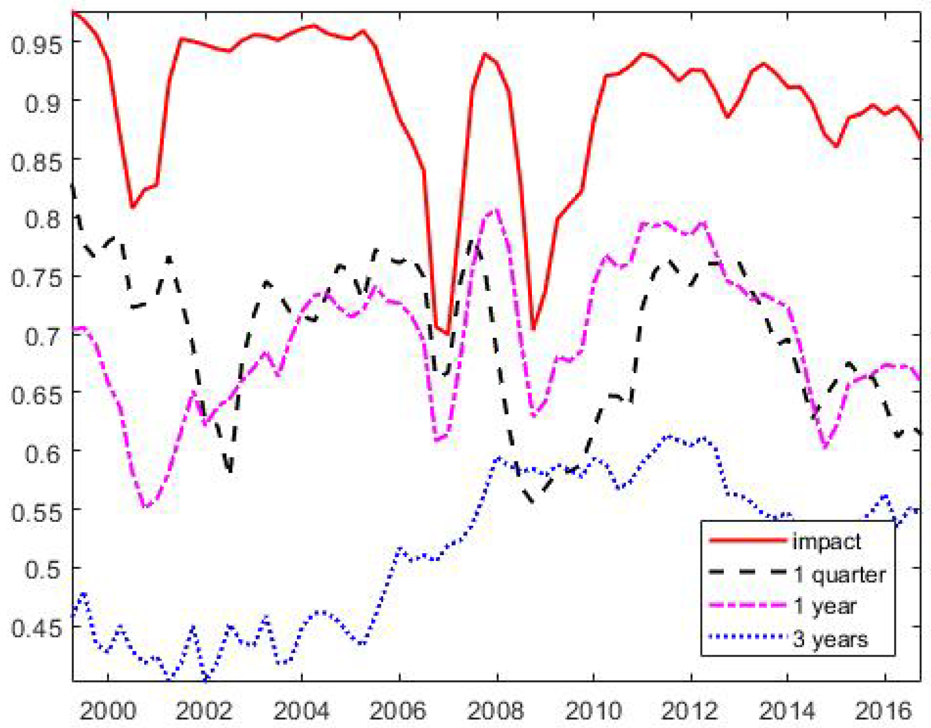
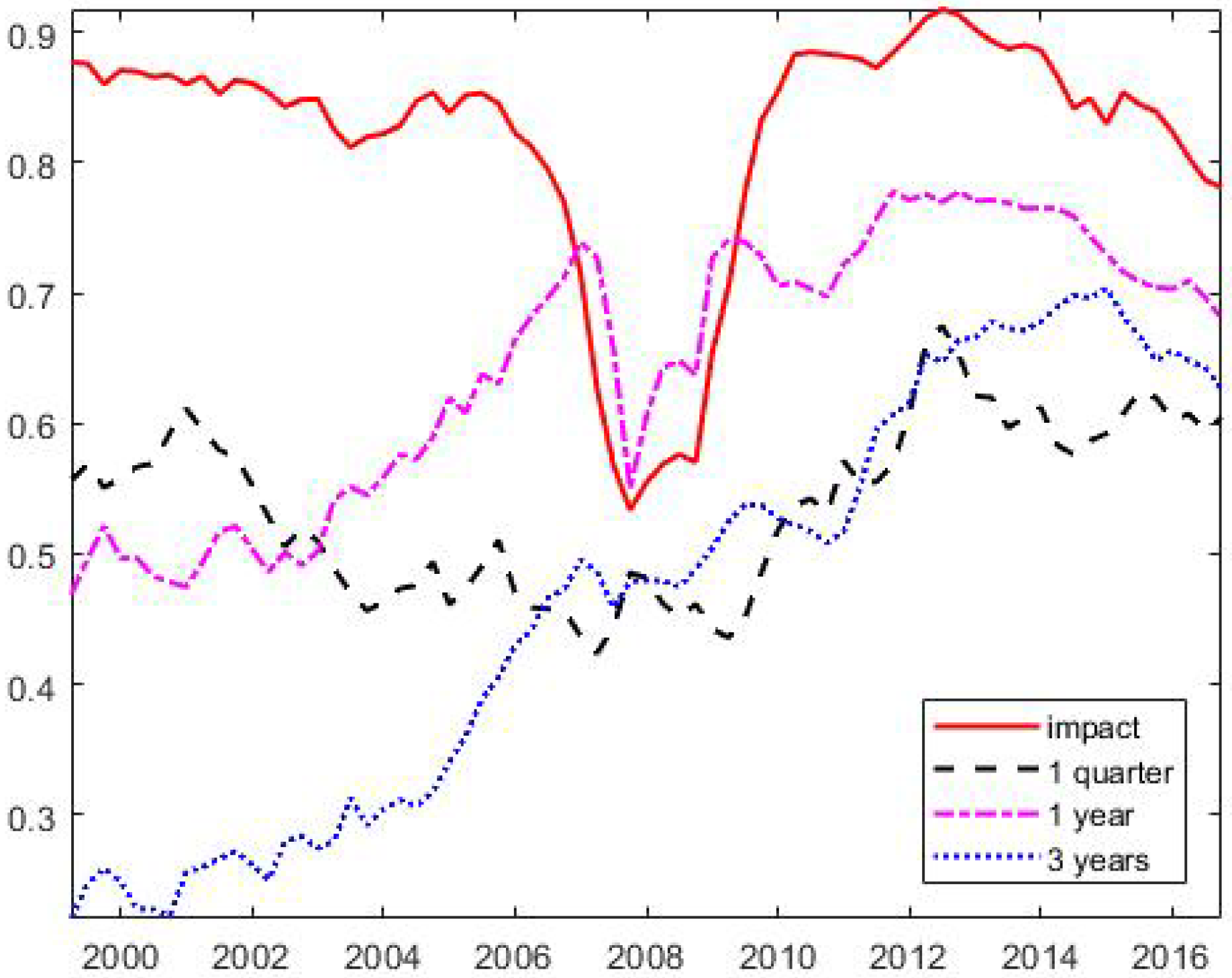
We discuss the results from several perspectives. We look at the time-varying impulse response functions for both asset prices, i.e., the prices of energy stocks, and for the bubbles in the sector (given by the difference between the asset prices as the underlying fundamentals, reflected in dividends). Results are shown in Appendix A (time-varying IRFs for asset prices), Appendix B (time-varying IRFs for bubbles), while the probabilities of a positive response are reported in Appendix C. We computed the mean response over our sample for the time-varying IRFs for horizons of 1 up to 20 periods ahead.

We found significant effects of monetary policy on asset prices for energy stocks, as well as on bubbles. The effects are stronger around the crisis period for both equity prices for energy and for the associated bubbles. This might suggest a high sensitivity of energy stock prices to the interest rate, as well as macro-financial conditions.

The sign of the energy stock responses is generally negative for both asset prices and bubbles (though there is an initial positive response by bubbles in the energy sector). The volatility around the crisis is quite high. This can be linked to the high drop in oil prices present at the end of 2008, a fact already studied in the literature.

Recent research (see [8]) has linked the volatility of oil prices during the crisis to macro-financial shocks. Furthermore, Ref. [24] found that the accelerated decrease at the end of 2008 is due to deleveraging by investing funds as well as reduced liquidity.

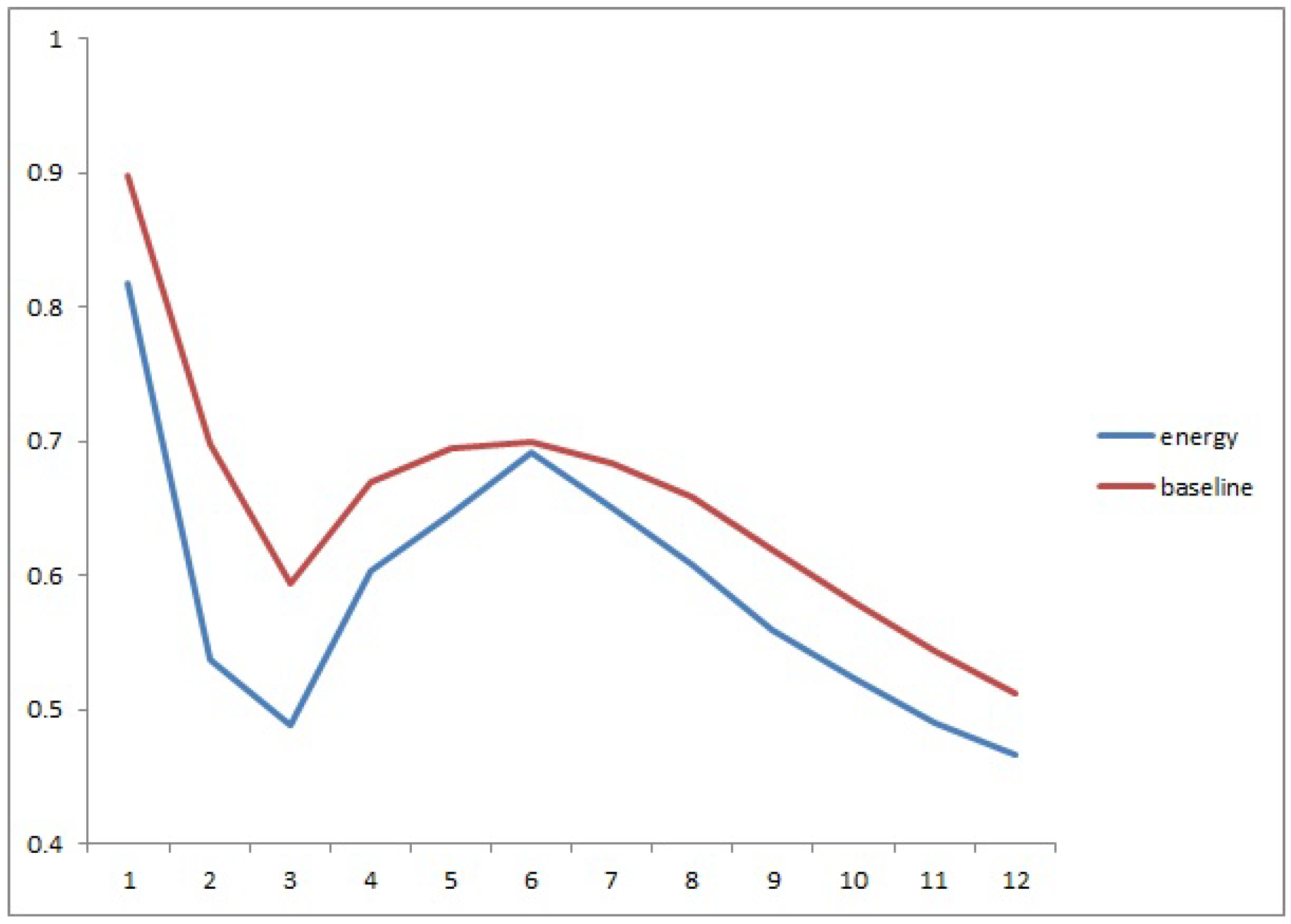
4.4. Comparing the Energy Sector to the Aggregate Economy

We further analyze the key results of our econometric analysis by comparing the results for the energy sector to those for the aggregate economy. The results for the aggregate case, i.e., the case of the United States, are based on an updated data sample of the original study by [14] that includes data up to the end of 2016 and considers the shadow interest rate. We have already compared the results obtained by using the shadow rate against those acquired when using the federal funds rate in a recent study, see [25], underlining that there are some substantial differences with respect to the sign of asset price responses. At the same time, the magnitude of the response of asset bubbles is much lower, (by 3 percentage points) when using the shadow interest rate.

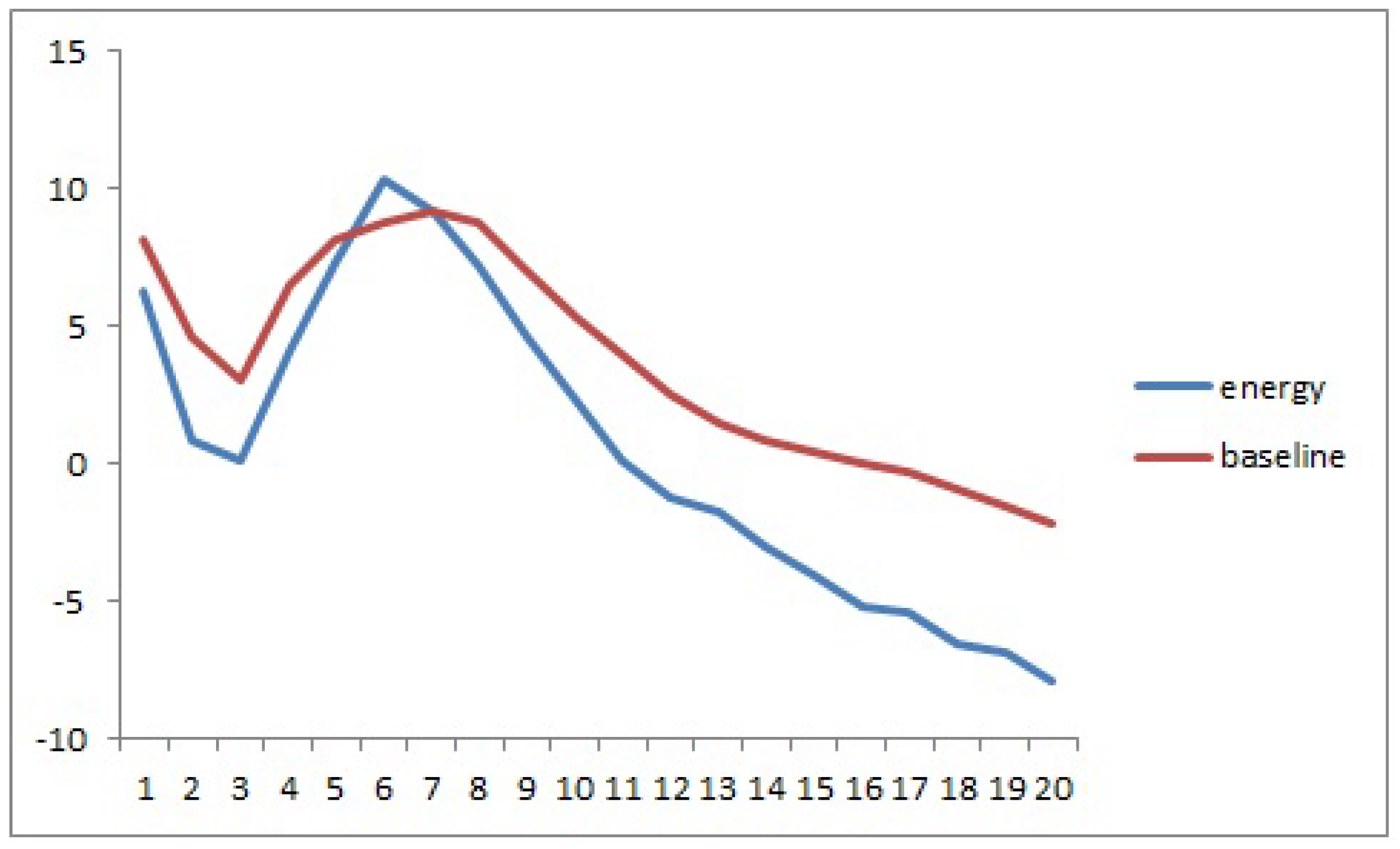
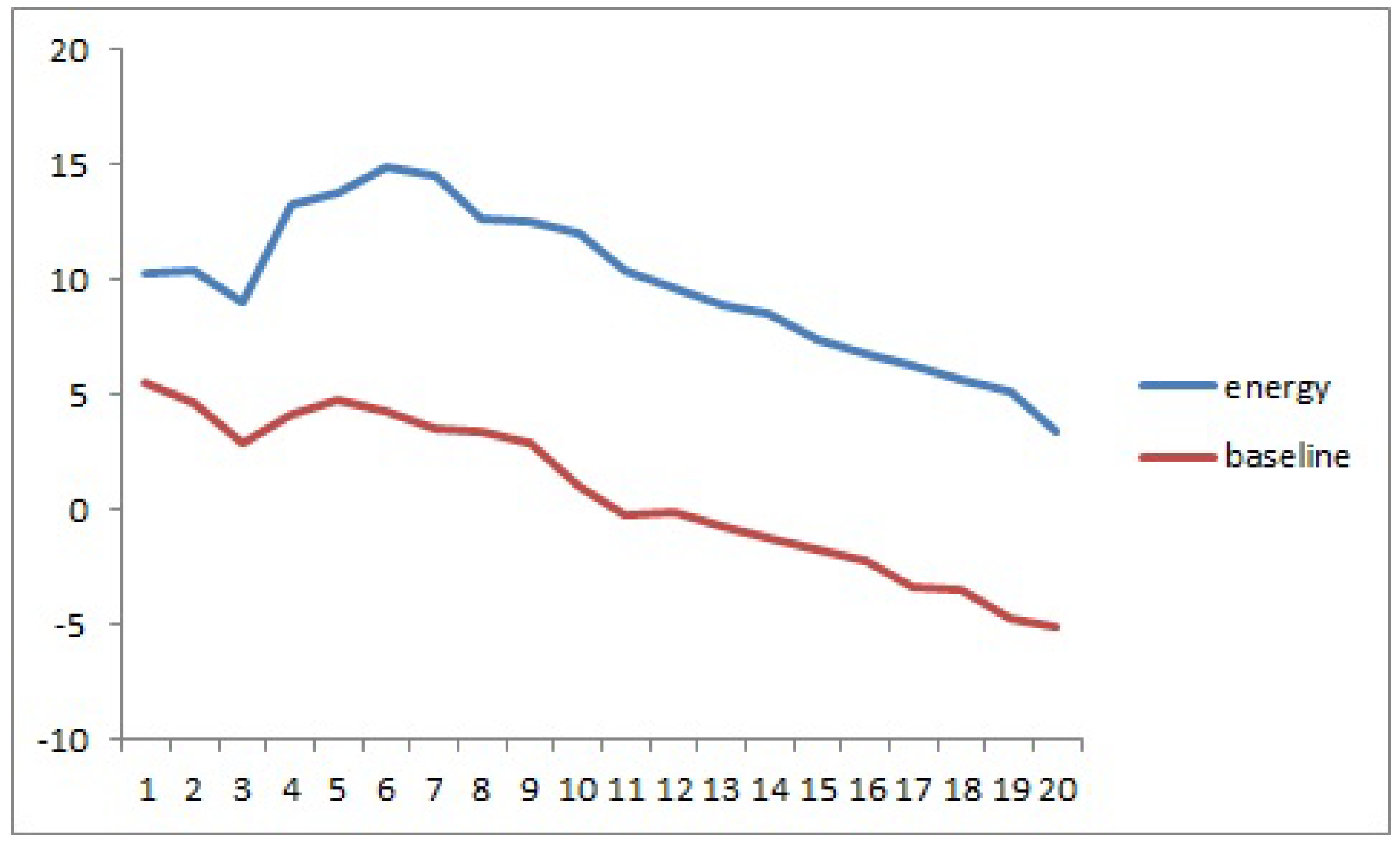
We found significant differences of the responses of the energy sector to monetary policy shocks. First, in terms of asset prices response, the effect of a positive shock in US monetary policy (a more restrictive monetary policy) leads to a lower and a more negative response relative to the aggregate economy (the gap is about two percentage points and it increases as the horizon of the IRF increases). We also found a very strong response during the financial crisis for both the aggregate and the energy sector, which can relate to previous research regarding the behavior of energy prices during the financial crisis, see again [8]. Second, with respect to bubble responses, the effects for the energy sector are initially positive but much weaker, and become negative after 3 years (12 periods). The effects for the aggregate economy remain slightly positive even towards the end of the sample (though the sign becomes negative in the last quarters). The gap between the two widens to over 5 percentage points as the horizon of the IRF increases.

Third, in terms of probability of a positive response of bubbles, we found a lower probability in the long run (of up to 20 quarters, i.e., 5 years) for the case of the energy sector. This is on average lower by 0.05 for the above-mentioned case.

In terms of magnitude, the results might appear to be quite strong. However, a few things should be underscored. First, the results are distorted by the fact that the sample for the time-varying IRFs is quite small, starting around 2000, including at the same time the last financial crisis (as well as the dot-com crisis in 2001). Second, there has been a very strong response of commodity prices at the beginning of the crisis which was surely reflected in the valuation of the energy firms. Third, the values of the IRFs indicate the growth in the returns of energy asset prices and the associated dividends. Moreover, related literature, such as [7], also found stronger effects for unconventional monetary policy shocks with respect to commodity prices.

4.5. Robustness

In this section, we consider an alternative measure of interest rate. Instead of the shadow rate, we use the long-term interest rate which is not deemed as sensitive to the zero lower bound. This has been used recently in the context of Phillips curve by [26]. The results are shown in Appendix D.

The use of long-term interest rates leads to several changes. First, for aggregate asset prices (that is, the stock market index for the aggregate case), the reaction becomes even more negative. We could note that the response of the energy sector is less negative, as it becomes less responsive than that of the aggregate market index.

Second, there are also some changes for the bubble responses. For the aggregate market, the reaction becomes negative, except for the first quarters. The response of bubbles in the energy sector is more stable and it stays positive.

The fact that the energy sector becomes less responsive for the long-term interest rate relative to the aggregate case might have to do with the way in which the market reacts to long-term versus short-term interest rates. The finding that the reaction of asset prices for energy prices remains about the same when using different interest rates is not really surprising. However, the switch from a short-term to a long-term interest rate leads to different bubble responses. This might be explained through the fact the bubbles are expected to be very sensitive especially to short run interest rates.

5. Discussion of Results

There has been a lot of debate in macroeconomics regarding the appropriate design of monetary policy in the wake of perceived asset bubbles. At the same time, researchers and policy makers in the field of energy economics have been puzzled by the high volatility of energy prices, as well as by their connection with potential bubbles in the energy sector, fueled by the increased use of advanced technology (for studies on the shale revolution or the boom in the green energy industry, see [18,27,28] or [19], to cite only a few contributions). In this paper, we tried to link the two and looked at the behavior of energy sector stocks following monetary policy shocks.

We analyzed both the responses of energy stocks and of the bubbles in the energy sector, measured by the difference between the market value of a stock and the underlying dividends. We also compared the dynamics for the energy sector with those for the aggregate US economy.

We found a significant difference between the energy sector and the aggregate US economy: the asset, as well as the bubbles responses to a positive monetary policy shock are more negative in the energy sector. This might suggest a high sensitivity of the US energy sector to changes in financing conditions.

We also considered as a robustness exercise, the use of the long-term interest rate, as advocated in the recent paper by [26]. Some results change, in the sense that the energy sector is less responsive, on one hand, and, at the same time, it reacts less than the aggregate stock market. The energy stocks continue to show a negative reaction to an unexpected increase in the monetary policy, while bubbles in the energy sector react now positively to shocks in the interest rate, pretty much along the results in [14] with respect to bubbles in the aggregate stock market.

Future studies could disaggregate the energy sector in the United States (or other countries) by using data on renewable energy or shale gas production. They could also look at the sources of financing that could uncover the main factors behind the sensitivity of energy stocks to monetary policy shocks.

The results of the article can also be regarded from the point of view of the extensive academic debate regarding the suitability of monetary policy reaction to asset prices dynamics, generally known as the “leaning against the wind” approach.

The mainstream view on the matter stipulates that monetary policy should not directly target stock prices. Under this view, its mission should reside in guarding the quality of the financial system and the price stability. These in turn can be achieved through inflation targeting even in the case of bubble-generated adverse effects [29].

A contrary perspective considers that central banks should modulate their policy to accommodate asset price bubbles. Its advocates argue that the intervention costs are usually lower than those deriving from the negative effects of bubble bursts.

Though extensive and in constant evolution, the specific literature is still far from reaching a conclusion on the above-mentioned debate. In addition to this, the case of energy markets has been generally ignored up to present in the corresponding literature. Future studies could perform more in-depth analyses about the formation of bubbles, while discussing the opportunity and limits of monetary policy measures (or other policy measures, including fiscal ones) that could counter bubble formation in energy market, see similar studies for the housing market, [30], or for the stock market, [14,25].