Abstract
A robust synergetic controller using different observers is developed to drive an anaerobic digestion biogas plant. The latter, a highly nonlinear process requires prohibitive cost sensors. Furthermore, some variables are downright immeasurable rendering control an intricate challenge. Only biogas flow which can be effectively measured, due to an easily integrated low cost sensor, will be considered available and used in this work. The proposed synergetic controller depends on immeasurable system states, thus observers will be used for state estimation. Substrate and biomass concentrations required in the synergetic control law will be obtained via three virtual sensors developed for a one stage fermentation process model. The model, used in this paper, consider the mechanization phase responsible for the biogas production because the objective is to improve the amount of methane produced. A simulation study of the biogas plant control with the proposed technique is compared to a classic PID (Proportional, Integral and Derivative) approach. Comparative studies are provided for observation and control via computer simulations.
1. Introduction
Anaerobic digestion (AD) is a biotechnological process widely used and a promising method to solve some energy and ecological problems in the agriculture and the agro-industry.
Production of biogas via anaerobic fermentation has been recently one of the most interesting research topics for two essential reasons: Elimination of organic waste (ecological aspect) and renewable power production (energetical aspect). The renewable energy produced in gas form is coined biogas in which methane constitutes the main component. This biotechnological process is described by a two stages reaction diagram expressed by a second order nonlinear model.
Biogas production by fermentation of organic material takes place in bioreactors tanks continuously stirred. The organic material is cleaned up by microorganisms producing biogas essentially composed of methane, carbon dioxide and compost in the absence of oxygen [1,2,3]. Different biogases with non-methane content can also be produced through this bioprocess [4] but will not be addressed in this work. Biogas is an additional source of energy which can possibly back up dwindling fossil fuels sources. Besides it has an indirect positive effect in the reduction of greenhouse gas emission, yet this complex process can become unstable in open-loop configuration and production of biogas may even exhaust itself if left without control.
Many factors enter in the biogas production among which the biodegradable organic matter content of the raw material subjected to anaerobic digestion, the sub-layer pH and temperature of the digester process [2]. An equally significant issue consists in the control approach applied to supervise the global biogas production process, which is to be addressed in this paper.
Implementation of the proposed synergetic control law based on the nonlinear system model entails the knowledge of the complete state vector of the system. Thus, it is necessary to reconstruct the state vector, using virtual sensors, i.e., observers, to generate the proposed control law. Observers are used in conjunction with a robust synergetic controller to address both robustness and variable unavailability issues in a tracking problem in a biogas production process.
This seemingly simple biogas process has revealed to be a challenging control topic, not only because it exhibits high nonlinearity features, but the controllers proposed in the literature rely on a problematic to a non-measurable system variable.
The contribution in this work lies in the fact that both biomass and substrate concentrations are estimated through different virtual sensors while the only really measurable variable relied upon, in the development of the control laws, is the output gas flow Q which is indeed readily available. Further enhancement comes from the synergetic control approach used, which is as robust as SMC (sliding mode control) but without the chattering problem.
Observers are used in conjunction with a robust synergetic controller to address both robustness and variable unavailability issues in a tracking problem in a biogas production process.
The rest of the paper is organized as follows: First, process description is briefly recalled followed by a brief synergetic control section. Introduction of three observers and their corresponding synergetic control laws of a biogas plant are then developed. The results of the simulation are presented and discussed in subsequent sections.
2. Process Description
2.1. Process Outline
These processes are carried out in continuously stirred tank bioreactors (CSTR); Figure 1 gives a basic layout of such a plant. The organic matter is depolluted by microorganisms into biogas (methane and carbon dioxide) and digestate in the absence of oxygen. The liquid medium contains cells and the substrates which are needed for the cell growth and cell production. The feed D is used to control the substrate concentration.

Figure 1.
Bioreactor basic schematics.
Well-mixed conditions are obtained through continuous stirring with a mechanical agitator. The produced cells are kept in the bioreactor where several control loops ensure that important process parameters, such as pH and temperature, stay close to specified operating conditions. The stirrer speed is often used to be kept constant as long as the liquid medium level is high enough; keeping good mixing in the reactor, the stirrer speed, N, does never fall never below a minimum value.
Cell metabolism can be described by different specific rates of growth μ, among which the Monod type will be used in this paper.
2.2. Process Modeling
Different mathematical models of AD exist in the specialized literature: One-stage, Three-stage and Five-stage model.
The model for the description of the AD process used in this study is the basic one-stage proposed in References [5,6,7,8] devoted to modeling anaerobic digestion obtained by fermentation.
The dynamics of the anaerobic digestion system represented by the model is illustrated by the following first order differential equations system:
is the concentration of the bacterial population (or biomass) (g/L), is the substrate concentration of complex organic materials in the bioreactor (g/L), is the inlet substrate concentration (g/L), and are positive constant yield coefficients. is the dilution rate and is the specific bacterial growth expressed by Equation (3). and are both expressed in day−1.
The measured output flow rate , in biogas (methane) is given by Equation (2). It’s expressed in L/day.
The last Equation (3) expresses the growth rate of methanogen bacteria that is obtained through the Monod model. is the maximum specific growth rate (day−1) and is a saturation parameter (g/L).
Specific values used in this work are given by:
are always positive values. is defined as the ratio of the flow to the volume of the bioreactor [1],
The plant model can be written in the following standard form:
where is the state vector defined by: , , is the control input: and .
The initial conditions are calculated at the equilibrium point given by L/day and day−1 [5]. By replacing in the Equation (1), we obtain at the equilibrium: and .
The bacterial concentration although small is never zero at startup, so: day−1.
Replacing by its value in Equation (3), leads to:
The resolution of this equation gives:
Replacing by its value, leads to:
The resolution of this equation gives:
2.3. Reference Process Modeling Analysis
The anaerobic fermentation process modeling has attracted interest as early as 1976 as can be seen in Reference [9] which tackled animal waste digestion modeling. Ensuing work of Bastin and Dochain [10] who proposed a one-stage reaction model for methane fermentation process formalized by a nonlinear second order system much used in the specialized literature. The methane fermentation process is a complex system with many time varying parameters, as well as variables that cannot be accurately measured if at all. Furthermore, the specific bacteria growth rate can take three different forms as proposed in Reference [10] and can greatly impact simulation results. Nevertheless, models based on Monod bacteria growth rate have been used extensively in biogas production control algorithms reinforced by Simeonov’s work [11] in which Monod, Contois, and Haldane bacteria growth rates were investigated in a thorough experimental study assessing positively the second order nonlinear model developed in Reference [10] and used in this paper. Indeed, the author in Reference [11] concludes that the model is suitable for control algorithms testing when considering continuous biogas fermentation.
This simple nonlinear model has been extensively used since then to evaluate control algorithms, such as extremum seeking [6], SMC [7,12,13,14], composite adaptive control [5], Hinf control [15], and fuzzy logic control [16].
More complex models, such as three and five stage reaction scheme models, exist, but only one-stage model using Monod’s growth rate form will be considered in this paper as continuous methane production is envisaged.
3. Bioreactor Control
CSTR is often a preferred way of methane production because the additional substrate is well integrated into agricultural cultures during the fermentation process.
3.1. Synergetic Control
Consider a nonlinear SISO dynamic process of any dimension described by Equation (4).
The development of the synergetic control starts with the choice of a macro variable [17,18,19], which contains the desired control constraints, as well as the performance specifications:
is the macro-variable and is a function of the state variables and the time chosen by the designer.
The synergetic control forces the system to evolve on the domain chosen by the user:
The macro-variable is forced to evolve in a desired way through a chosen constraint indicated by Equation (10) according to the desired dynamics for the evolution of .
T is the convergence speed. Differentiation of the macro-variable gives:
The substitution of Equation (10) in Equation (9) leads to writing:
By solving Equation (11) the control law can thus be obtained as a function of the state vector, the macro-variable, the convergence speed and time.
Applying this approach to the underlying bioprocess starts by a choice of a synergetic macro-variable defined by:
where represents constant desired gas flow output.
Expressing the constraints of Equation (9) with the synergetic macro-variable defined by Equation (13) gives:
Calculation of :
Basic simplification steps lead to:
Using:
One can rewrite Equation (17) as:
Replacing by its value:
Porting Equation (19) in Equation (14), gives:
Straightforward steps lead to the controller of Equation (22):
It is to be noted that biomass concentration is never null.
Synergetic control stability proof
Stability of the closed loop system can be proved using the following Lyapunov function:
The derivative of the Lyapunov function is given by:
From the constraints of Equation (9) one obtains:
Replacing Equation (25) in Equation (24) leads to:
The closed loop system is thus stable under synergetic control.
3.2. PID Control
A standard PID (Proportional, Integral and Derivative) controller, widely used in industry [20] will be used in this paper with the aim of comparison. The controller in this case can be expressed by the following relation:
As defined before for the fermentation process expresses the error between the desired biogas output flow and the actual plant output .
The PID gains used in this paper are taken from reference [5] for comparative purposes.
The desired trajectory of the output is selected in the form of steps of increasing heights for 200 days [5]:
0.45 L/day before 30 days; 1 L/day between 30 days and 60 days; 1.5 L/day between 60 days and 90 days; 1.8 L/day between 90 days and 120 days; 2.1 L/day between 120 days and 200 days.
3.3. Simulation Results
Simulation is carried out under the environment Matlab/Simulink for a 200 days period using PID and synergetic controllers. The system is simulated using Equations (1)–(3), (5), (6), (22) and (27), process parameters, given in Section 2.2, and PID parameters, given in Section 3.2.
It is evident, as can be noted from Figure 2, that good tracking occurs under both controllers, using the parameters of the PID mentioned above given in Reference [5] and T = 0.01 for the synergetic approach. It is observed that PID control provides a faster response than the proposed approach at transitions and in the event of reference variations. Besides PID control presents elevated peaks at transitions. Overall synergetic performance, such as response time and steady-state error are improved compared to PID.

Figure 2.
Time evolution of biogas flow rate under PID control and synergetic control for T = 0.01.
On the other hand, PID control signal requires much more dilution rate D at transitions time than when synergetic control is used as can be seen in Figure 3c. Indeed, the highest level of required flow rate (6.1/day) for synergetic control occurs at 120 days but reaches a much higher level (61/day) for PID control lasting for 0.01 day(≈15min).Thus, the value of these peaks is more reasonable with the synergetic control. These results have been obtained making the assumption that the complete system state vector was readily available and used in the control laws used; however, the state vector is not completely measurable. A more realistic approach would be therefore to rely on an observer devoted to the estimation of both concentrations X and S. Different observers are introducing in the ensuing sections and simulation results discussed.

Figure 3.
Control signal evolution (a) under synergetic control for T = 0.01 (b) under PID control (c) under PID control zoomed section.
4. Observers Based Control
In practice it is not possible to measure on-line the different bacterial concentrations or their specific growth rates. Other biochemical variables important for the AD processes are too costly to be measured. In practice, only the biogas flow rate can be easily measured on-line. One of the most promising ways to solve this problem is the design of software sensors for estimating biochemical variables on the basis of an AD mathematical model and some easily measured process parameters [8,13,21].
Hence in this paper, only the use of reliable gas sensor will be exploited in the control of this biotechnological process, other required state variables will be estimated through different observers (Figure 4).

Figure 4.
Control based on observer state estimation.
As with most applications, biogas production does not offer readily accessible variables for the direct measure to empower developed control law; the latter requires nevertheless high cost sensors not often accurate or always available. These drawbacks on top of difficulties in maintenance and eventual induced stochastic errors are often mitigated by the use of algorithms coined observers designed to replace hard sensors efficiently. Such observers are used to estimate substrate and biomass of the bioreactor previously described.
Different observers for this kind of process have been proposed in the literature but these observers rely on measurements made on the substrate which is not only very costly but may be less efficient than gas flow measurement.
Furthermore, it is practically impossible to measure on-line different bacterial concentrations or specific growth rates [21]. Other biochemical variables are too expensive to be measured. In practice, the biogas flow rate sensor is not expensive and it is easily integrated in the process. So, it’s the only measured variable and virtual sensors are used in the following section to estimate bacterial and substrate concentrations variables.
4.1. Observer with Linear Feedback
Observer dynamics are given by Equation (28). The estimated state vector is computed using the plant model, to which a linear corrective term is added [8], to ensure the convergence of the state estimate to the system state x.
Defining the output estimation error then the observer may be written as:
where, is the observer gain.
Using the observer above onto the biogas process, where , leads to Equation (29). Biomass, substrate concentration and biogas flow rate estimations are given by Equation (29):
Global stability proof
After observation, defined in the control section becomes which can be written . Steady state as has already been proven so .
Observation errors are given by Equation (30):
Introducing a new variable given by Equation (31)
The error dynamics can be rewritten as:
Choosing the following Lyapunov function:
Its derivative is given by:
Making use of Equation (32) into Equation (34) leads to:
Noting that:
So:
Porting Equation (37) into Equation (35) gives:
This can be written as:
With:
For it is necessary that the symmetric matrix be positive definite.
For positive definite, it is necessary that the main minors of are positive [22].
For simplification purpose the following steps are taken:
This leads to:
Stability is thus guaranteed with gains defined by Equations (42) and (43).
A nonlinear robust observer based on sliding mode techniques will be recalled in the ensuing section.
4.2. Sliding Mode Observers
As stated above only Q measurements are available, estimates of both biomass and substrate concentrations will be obtained via a first order sliding mode observer.
4.2.1. First Order Sliding Mode Observer (FOSMO)
The sliding mode observer [23,24] is given by:
The used term of correction is proportional to the discontinuous function sign applied to the output error where is defined by:
Applying FOSMO to the biogas process lead to:
where , and are observer gains and is the sliding surface [23,24].
Global stability proof
Introduction of the variable . defined by Equation (31), Equation (32) can be written for this observer as:
Choosing Lyapunov function , Equation (33), and proceeding in the same manner as before for Equations (34) and (35), one can write:
Eliminating the sign function using .
And noting that is small but not null lead to:
For , it is necessary that the matrix be positive definite.
For positive definite, it is necessary that the main minors of be positive.
Some simplification steps taken before are carried out a gain:
The gain may be obtained by Equation (51):
Stability is thus guaranteed with gains defined by Equations (50) and (51).
4.2.2. Sliding Mode Observer with PD Based Surface
In this section, the proposed sliding surface is PD (Proportional derived). Proceeding as before, the observer gain term is replaced by for the first state variable and for the second state variable .
where is the new sliding surface [25].
Stability proof is similar to Section 4.2.1.
Interested readers in the observability of the bioprocess are referred to the excellent and detailed work of Selişteanu [13].
5. Simulation and Results
For the bioprocess represented by Equations (1)–(3), simulation results are presented for the synergetic controller given by Equation (24), the process parameters used in Section 2, , , , , , , , .
The observer based synergetic control is obtained by replacing by , by , by , as well as by in Equation (22) for all the virtual sensors written as (53):
Simulation of the biogas process control using:
a) Linear feedback observer based synergetic control.
Starting with as shown in Figure 5a good tracking occurs under the proposed observer based synergetic controller. As previously found the control signal in Figure 5b although vitiated with peaks at transitions show much lower magnitude values as opposed to the PID approach. Rapidly dwindling estimation errors for both concentrations and are given in Figure 5c,d.

Figure 5.
Linear feedback observer based synergetic controller. (a) Time evolution biogas flow rate; (b) control signal evolution; (c) error of the bacterial concentration evolution; (d) error of the substrate concentration evolution.
b) First order sliding mode observer based synergetic control.
c) Sliding mode observer with PD based surface based synergetic control.
Simulation results for biogas output flow rate, biomass and substrate concentration obtained for three observers under the proposed control approach used are given in Figure 5, Figure 6 and Figure 7 showing good overall tracking performance. Figure 5a, Figure 6a, Figure 7a show that the three observers act in the same way on biogas flow rate evolution. Figure 5b, Figure 6b and Figure 7b show the control effort necessary to achieve the desired tracking. It is to be noted that the magnitude of the synergetic control signal is much lower than under PID control for all observers. Estimation errors magnitude orders are similar for the three observers used as can be seen in Figure 8a, and faster response time for the SMO based proposed control technique this comes out with chattering as expected. As anticipated response time using the two type of SMO is faster than that obtained with the linear feedback observer (Figure 8a).

Figure 6.
Anaerobic digestion first order sliding mode observer based synergetic controller. (a) Biogas flow rate; (b) control signal evolution; (c) estimation error of the concentration of the bacterial population X; (d) estimation error of the concentration of the substrate S.
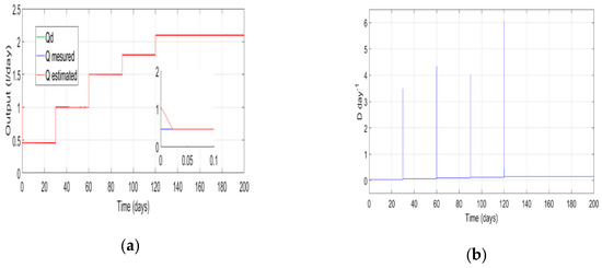

Figure 7.
Anaerobic digestion sliding mode observer with PD based surface under a synergetic controller. (a) Biogas flow rate evolution; (b) control signal; (c) error of the concentration of the bacterial population X; (d) error of the concentration of the substrate S.
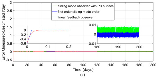

Figure 8.
Comparison between three observers (a) Error evolution of biogas flow rate measured, and biogas flow rate estimated with the virtual sensors; (b) evolution of the real biomass and estimated biomass with three observers; (c) evolution of the real substrate and estimated substrate for three observers.
Figure 8b,c shows the chattering phenomenon for the two sliding mode observers. Switching/chattering of sliding mode observation signals crossing the sliding mode surfaces is an important characteristic in all current sliding mode observation systems. To eliminate the chattering, the property of the zero-error convergence is to replace the sign function by the sigmoid function in sliding mode observation and also control signals. Nevertheless, this phenomenon is less important when introducing PD surface.
6. Conclusions
Among the multiple sources of renewable energy, biogas is produced by anaerobic digestion. The controlled use of this natural phenomenon makes it possible to recover organic waste while producing biogas that can replace natural gas for many applications.
In this paper, the synergetic approach has been proposed for trajectory tracking in the context of the fermentation of organic waste in a biogas bioreactor.
Contrarily to many other published works in which bacterial and substrate concentrations are used in the control algorithms, in this work a more realistic approach, based on effectively measurable biogas flow rate, is developed based on synergetic control methodology.
Simulation results compared to a typical PID control show not only the improvement in response time and static error, but a drastic reduction in the control signal occurs as well.
Synergetic control depends on the substrate and biomass concentrations that are not easily measurable, that which justifies the use of virtual sensors. Thus, three observers have been used in conjunction with the proposed approach in tracking a nonlinear trajectory showing acceptable performances. Substrate concentration estimation allows possible to estimate the growth rate of methanogen bacteria.
Finally, we summarize the perspectives in four main areas:
- Optimization of the control parameters via meta-heuristic techniques;
- Use of the three and five stage process models;
- Use of higher order sliding mode observers in order to eliminate the chattering phenomenon caused by the sliding mode observers used;
- Experimental validation should be carried out to assess the soundness of the studied control algorithm and the effectiveness of all the proposed observers.
Author Contributions
H.B. and S.S. built the simulation model, M.N.H. proposed the controller K.N.M. and A.N. proposed the observers and studied the stability. All the authors analyzed the results and revised the paper.
Conflicts of Interest
The authors declare no conflict of interest.
References
- Tan Deublein, L.; Steinhauser, A. Biogas from Waste and Renewable Resources; Wiley-VCH: Weinheim, Germany, 2008; ISBN 978-3-527-31841-4. [Google Scholar]
- Simeonov, I.; Naamane, A. Hybrid mathematical modeling and PH control of anaerobic waste waters treatment processes. In Proceedings of the AIS’2002, Lisbon, Portugal, 7–10 April 2002. [Google Scholar]
- Achiraya, J.; Kornpong, V.; Malinee, L.; Sumaeth, C. Three-stage anaerobic sequencing batch reactor (ASBR) for maximum methane production: Effects of COD loading rate and reactor volumetric ratio. Energies 2018, 11, 1543. [Google Scholar]
- Cermy, M.; Vitezova, M.; Vitez, T.; Bartos, M.; Kushkevych, I. Variation in the distribution of hydrogen producers from the clostridiales order in biogas reactors depending on different input substrates. Energies 2018, 11, 3270. [Google Scholar] [CrossRef]
- Wang, H.P.; Kalchev, B.; Tian, Y.; Simeonov, I.; Christov, N.; Vasseur, C. Composed adaptive control for a second-order nonlinear model of a biotechnological process. In Proceedings of the 19th Mediterranean Conference on Control and Automation, Corfu, Greece, 20–23 June 2011. [Google Scholar]
- Wang, H.P.; Krstic, M.; Bastin, G. Optimizing bioreactors by extremum seeking. Int. J. Adapt. Control Signal Process. 1999, 13, 651–669. [Google Scholar] [CrossRef]
- Kravaris, C.; Savoglidis, G. Tracking the singular arc of a continuous bioreactor using sliding mode control. J. Frankl. Inst. 2012, 349, 1583–1601. [Google Scholar] [CrossRef]
- Ramjug-Ballgobin, R.; Rugooputh, H.C.S.; Busawon, K.; Binns, R. Observer-based control for biomass regulation in wastewater treatment plants. In Proceedings of the International Conference on Computing, Communication and Security, Pamplemousses, Mauritius, 4–5 December 2015. [Google Scholar]
- Hill, D.T.; Barth, C.L. A dynamical model for simulation of animal waste digestion. J. Watt. Pol. Contr. Fed 1977, 49, 2126–2143. [Google Scholar]
- Bastin, G.; Dochain, D. On-line Estimation and Adaptive Control of Bioreactors; Elsevier Science Publishers: Amsterdam, The Netherlands; New York, NY, USA, 1990; ISBN 0-444-88430-0. [Google Scholar]
- Simeonov, I. Mathematical modeling and parameters estimation of anaerobic fermentation processes. Bioprocess Eng. 1999, 21, 377–381. [Google Scholar] [CrossRef]
- Tham, H.J.; Ramachandran, K.B.; Hussain, M.A. Sliding mode control for a continuous bioreactor. Chem. Biochem. Eng. Q. 2003, 4, 267–275. [Google Scholar]
- Selişteanu, D.; Petre, E.; Rasvan, V.B. Sliding mode and adaptive sliding-mode control of a class of nonlinear bioprocesses. Int. J. Adapt. Control Signal Process Wiley Inter Sci. 2007, 21, 795–822. [Google Scholar] [CrossRef]
- Veluvolu, K.C.; Soh, Y.C.; Cao, W. Robust observer with sliding mode estimation for nonlinear uncertain systems. Iet Control Theory Appl 2007, 5, 1533–1540. [Google Scholar] [CrossRef]
- Kalchev, B.; Christov, N.; Simeonov, I. Output-feedback Hinf control for a second-order nonlinear model of a biotechnological process. Compt. Rend. Acad. Bulg. 2011, 64, 125–132. [Google Scholar]
- Arulmozhi, N. Bioreactor control using fuzzy logic controllers. Appl. Mech. Mater. 2014, 573, 291–296. [Google Scholar] [CrossRef]
- Mehdi, L.; Barazane, L. Synergetic speed control of squirrel motor drives. Rev. Room Sci. Tech Électrotechn. et Énerg. 2016, 61, 111–115. [Google Scholar]
- Kolesnikov, A.; Veselov, G. Modern Applied Control Theory: Synergetic Approach in Control Theory; TSURE Press: Taganrog, Russia, 2000. [Google Scholar]
- Bouchama, Z.; Essounbouli, N.; Harmas, M.N.; Hamzaoui, A.; Saoudi, K. Reaching phase free adaptive fuzzy synergetic power system stabilizer. Int. J. Electr. Power Energy Syst. 2016, 77, 43–49. [Google Scholar] [CrossRef]
- Visioli, A. Practical PID Control; Springer: London, UK, 2006. [Google Scholar]
- Simeonov, I.; Diop, S.; Kalchev, B.; Chorukova, E.; Christov, N. Design of Soft-Ware Sensors for Unmeasurable Variables of Anaerobic Digestion Processes; Bulgarian Academy of Sciences, Science and Engineering: Sofia, Bulgaria, 2012; pp. 307–311. [Google Scholar]
- Gilbert, G.T. Positive definite matrices and Sylvester’s criterion. Am. Math. Mon. 1991, 98, 44–46. [Google Scholar] [CrossRef]
- Jaballah, B.; M’sirdi, K.N.; Naamane, A.; Hassani, M. Estimation of vehicle longitudinal tire force with FOSMO & SOSMO. Int. J. Sci. Tech. Autom. Control Comput. Eng. 2011, 5, 1516–1531. [Google Scholar]
- Rabhi, A.; M’sirdi, K.N.; Naamane, A.; Jaballah, B. Estimation of contact forces and road profile using high order sliding modes. Int. J. Veh. Auton. Syst. 2010, 8, 23–38. [Google Scholar] [CrossRef]
- Edwards, C.; Spurgeon, S.K.; Patton, R.J. Sliding mode observers for fault detection and isolation. Automatica 2000, 36, 541–553. [Google Scholar] [CrossRef]


© 2019 by the authors. Licensee MDPI, Basel, Switzerland. This article is an open access article distributed under the terms and conditions of the Creative Commons Attribution (CC BY) license (http://creativecommons.org/licenses/by/4.0/).