Model Predictive-Based Secondary Frequency Control Considering Heat Pump Water Heaters

Abstract

The extensive development of renewable energies in power systems causes several problems due to intermittent output power generation. To tackle the challenge, demand response contribution to ancillary service is currently well recognized under the smart grid infrastructure. The application of the heat pump water heater (HPWH) as a controllable load in primary frequency control is well presented in the literature; however, the motivation of this paper is to use HPWHs for secondary frequency control. To this end, a model predictive control (MPC) method for a two-area power system incorporating HPWHs to contribute to secondary frequency control is proposed in this paper. A detailed model of HPWH is employed as a controllable load to control the power consumption during water heating. The MPC method predicts the future control signals using a quadratic programming-based optimization. It uses the system model, past inputs and outputs, as well as system control signals to predict the next signals. The effective performance of the proposed method for the two-area power system with HPWH is demonstrated for different scenarios of load changes, intermittent renewable power generation and parameter variations as the sensitivity analysis.

1. Introduction

Load frequency control (LFC) is responsible for frequency regulation in power systems after any imbalances between generation and load demand. In power systems, the LFC is utilized at two levels or loops: primary control and secondary control [1]. Automatic generation control (AGC) is the mechanism that supervises the secondary frequency control in a power system. Traditionally, conventional power plants such as thermal plants participate in both levels of LFC [2]. However, the increased fossil fuels price and air pollution concerns cause attenuation of the role of conventional generation plants in frequency control [3]. Renewable energy resources like wind turbines and solar photovoltaic can participate in frequency control [4,5]. Since the active power output of renewable energies is intermittent, they should operate near their highest capacity for efficient generation [6]. Therefore, there is not enough reserve for efficient contribution to LFC from renewable energy resources. Flexible AC transmission systems are the other components that can contribute to secondary frequency control [7]. Meanwhile, the high cost of these components is a barrier to their application.

Owing to the smart grid infrastructure in modern power systems, the demand response contribution to frequency control is currently well recognized [8]. Among the different types of demand response appliances, electric vehicles (EVs) and heat pump water heaters (HPWHs) are the most significant controllable loads. The charging/discharging process of EVs can be controlled using bidirectional inverters by appropriate control signals in designed stations to contribute to LFC. In HPWH, the power consumption of the appliance can be controlled during water heating through appropriate control signals of the control centre. Frequency control using EVs is well addressed in the literature for primary control [9,10] and secondary control [11,12,13] of power systems. Meanwhile, there is a lack of study of the HPWH contribution to LFC in power systems.

A detailed model is developed for HPWH under smart grid infrastructure in [14] for primary frequency control. In [15], the participation of HPWH in primary frequency control of a single-area power system has been proposed along with EVs and battery energy storage without any secondary loop controller. As is seen, the application of HPWH as a controllable load in primary frequency control has been presented in the literature; however, the motivation of this paper is to use HPWHs for secondary frequency control. In [16], HPWHs have been developed for secondary frequency control of a multi-area power system; however, a simple model has been employed for HPWH. In this study, a model predictive control (MPC) approach is used for HPWH to contribute to the secondary frequency control of a two-area power system.

MPC is a control approach based on the state-space model prediction of the system. Indeed, MPC provides inputs to the system based on the model and optimization. The objective function is defined by the system designer, and quadratic programming is used for optimization. The MPC method is successfully applied for frequency control of power systems [17,18,19]. The MPC application is also reported for LFC in multi-area power systems with: wind turbines [20], electric vehicles [21], superconducting magnetic energy storage [22], photovoltaic generation [23] and a multi-terminal high voltage direct current-connected grid [24]. Meanwhile, application of MPC in LFC with HPWH is not addressed in the literature.

The main contributions of this paper are:

(1)

The effect of merging HPWHs on the dynamic response performance of multi-area power systems is investigated.

(2)

MPC is designed for an LFC of a hybrid power system including a thermal generator, hydro power, a gas unit and HPWH.

(3)

A state-space model of the two-area power system including a detailed model of HPWH is presented and used in the design process.

(4)

The effectiveness of MPC with the participation of HPWHs is examined under three disturbance scenarios including: step load change, combined scenario of intermittent renewable power generation and random load change, as well as parameter variations.

The remainder of this paper is organized into five sections. Section 2 explains the aggregated model of HPWH and its structure in detail. The state-space model of the power system with generation units and HPWH is addressed in Section 4. The MPC description as a control technique is provided in Section 5. Simulation results in three different scenarios are demonstrated in Section 5. Finally, the conclusion in Section 6 closes the paper.

2. Heat Pump Water Heater

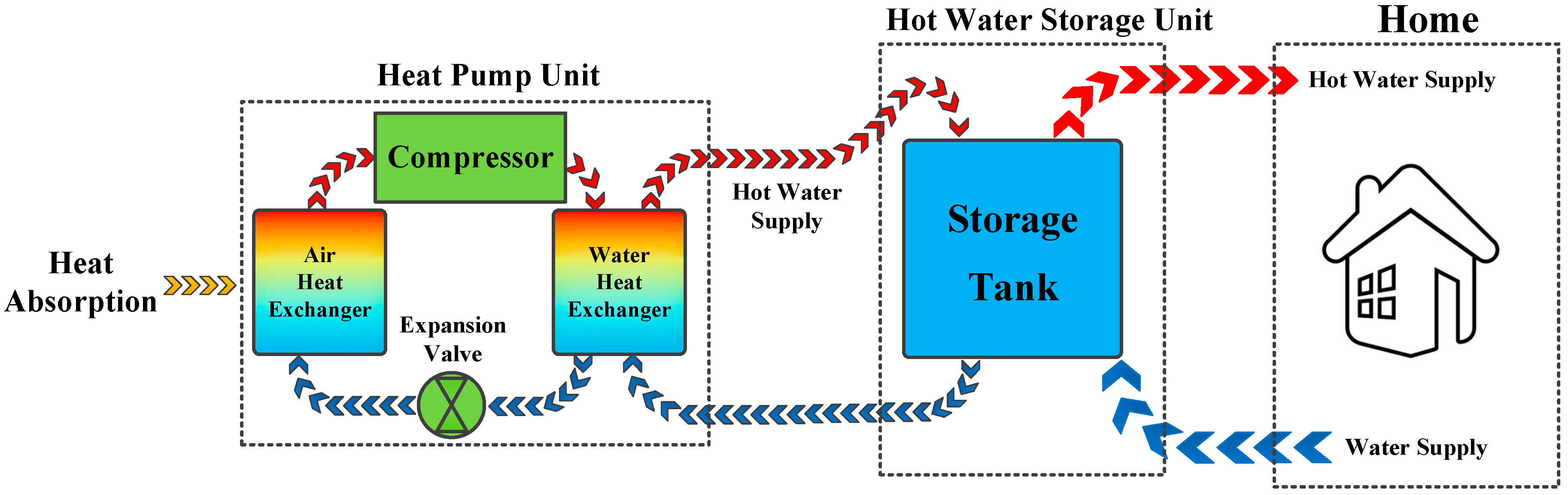
An HPWH absorbs warmth from the surrounding air and transfers it to heat water. Hence, it is also referred to as ‘air-source heat pump’. A tank is used in the HPWH structure to store the amount of hot water used in a day. Figure 1 demonstrates the schematic diagram of the heat pump water heater. It operates on electricity, but is roughly three-times more efficient than a conventional electric water heater [25]. Actually, the heat pump uses a small amount of energy to move heat from one location to another. Therefore, heat pump water heaters are known as high-efficiency and energy-saving appliances. HPWHs provided around three percent of Australian households’ hot water in 2012 [25]. In Japan, it is expected that the numbers of HPWHs will be around 10 million in 2020 [15].

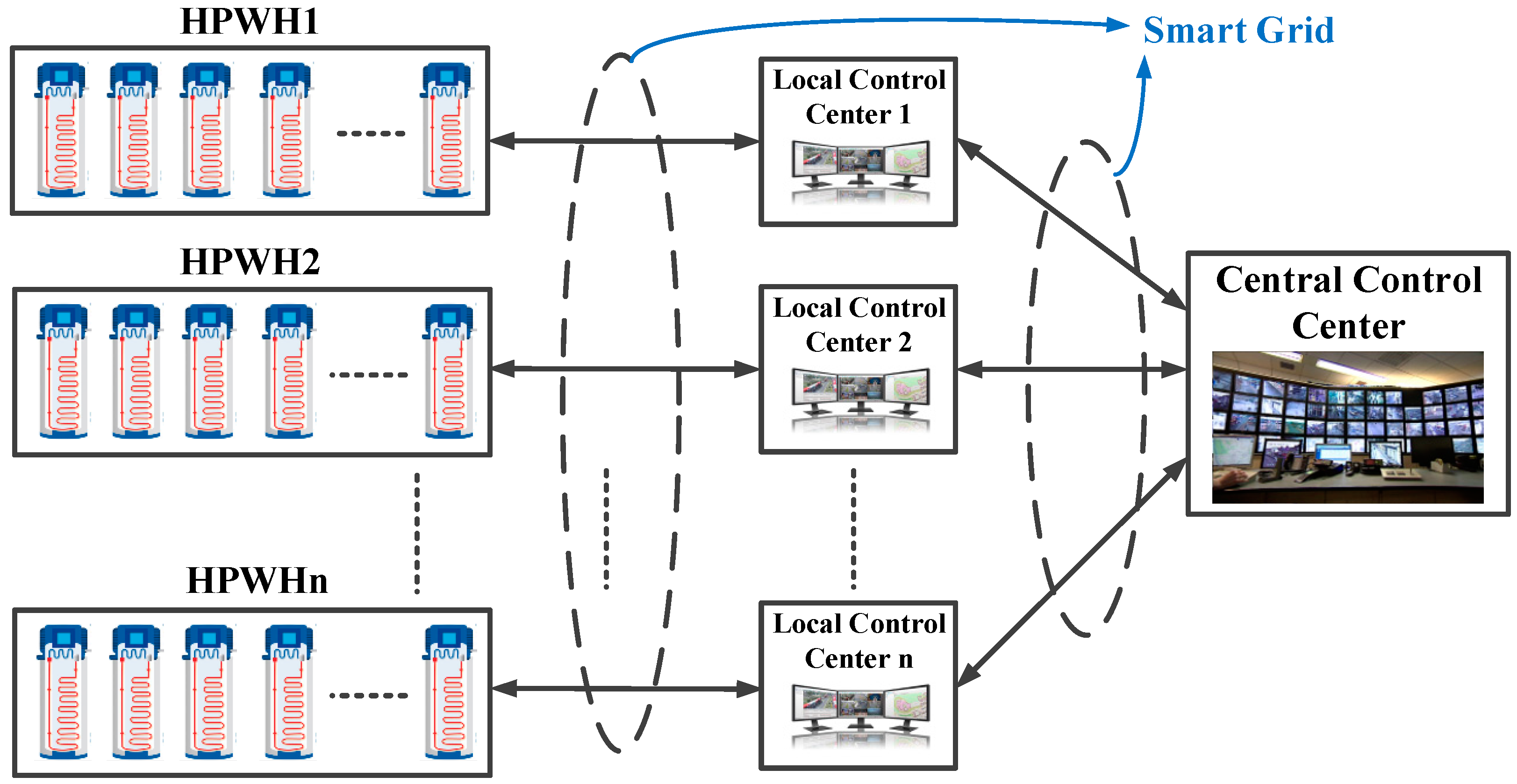
The main point about HPWH is that the power consumption can be controlled during operation. This means that by providing the appropriate control signal, the power consumption can be decreased or increased. The hierarchical control of HPWHs is shown in Figure 2. There is a bidirectional relation between the central control centre and the local control centre; also, the relation between the local control centre and HPWHs is bidirectional. The central control centre determines the amount of power for frequency control, and the local control centre sends the available power through all HPWHs in the system. In the lower layer, the local control centre collects the data of available HPWHs for frequency control. Moreover, it can send the control signal for HPWHs. All these connections are possible under the smart grid concept, which uses information and communication technology. The recent smart grid control approaches for central and distributed levels of HPWHs were investigated in [26].

3. System Dynamics

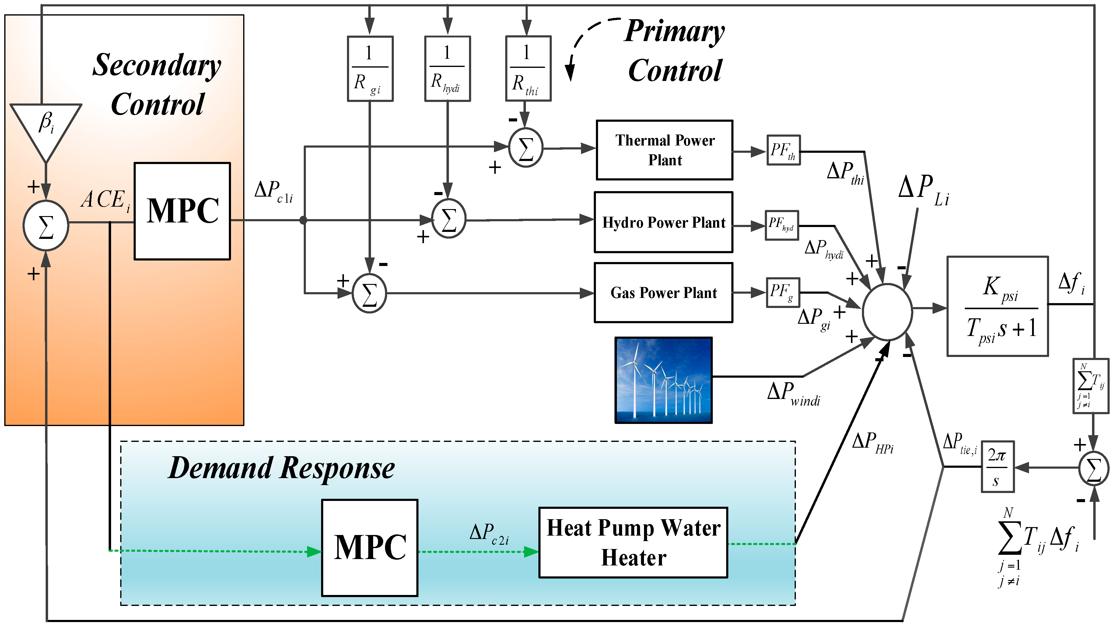
In a multi-area power system, the frequency performance is not just improved by the generators in a specific area; it is also improved by the generators in other areas through the tie-line power. A two-area power system including thermal, hydro and gas generation units in each area is considered as the system under study. HPWHs are added to both areas. Figure 3 shows a sample control area (i) of the considered power system. The system dynamics (state-space model) should be represented clearly in order to apply the MPC approach to the system. To follow the two-area power system model, a block diagram representation of the considering thermal, hydro and gas units and HPWH is shown in Figure 4. To be more accurate, the generation rate constraint (GRC) nonlinearity is also applied in the models of thermal and hydro units. All the considered parameters have been defined in the Nomenclature Section.

In the following, the state-space model for each of the traditional units and HPWH are outlined.

3.1. HPWH State-Space Model

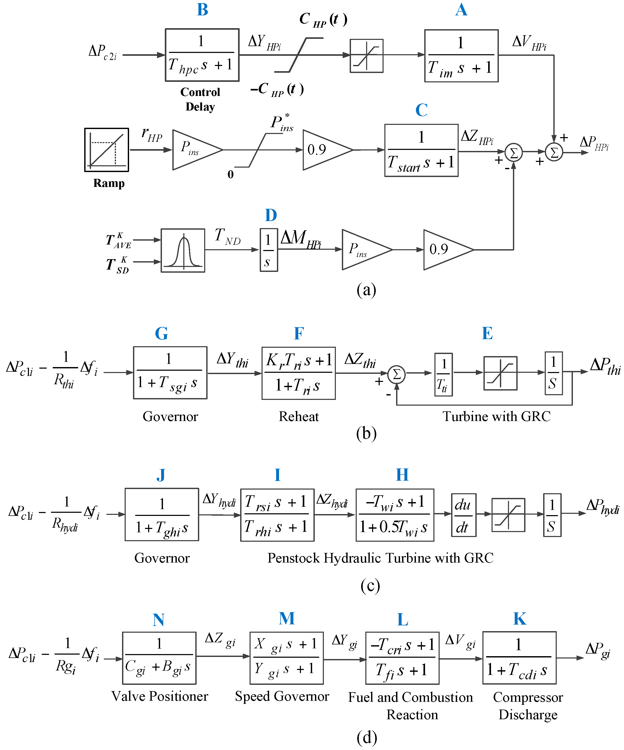
The detailed model of HPWH was provided in [15], which is used in this study. In [15], the secondary frequency control, which should be utilized by the desired controller, was ignored by the authors. In the model, it is assumed that HPWHs can only participate in frequency control at the range of 90 ± 10% of their rated power consumption in order to maintain efficiency. The state-space model in Figure 3a is the aggregated model, which shows the dynamic behaviour of HPWH for one local group. The input signal is the area control error (ACE), which is the summation of frequency deviation in the power system area and tie-line power deviation. The MPC block is added as a controller to contribute to HPWH in the secondary frequency control of the power system. Different time delays including control delay (T_hpc), induction motor delay (T_im) and start delay (T_start) are considered in the model and applied in the MPC design process. The power consumption represents the total power consumption of the local group. The ramp function is for the start-up power consumption, which is 90% of the total power consumption of HPWH. P_i is the total rated power consumption of the installed HPWHs. $T_{AVE}$ and $T_{SD}$ demonstrate the average value and the standard deviation of the estimated heating period of HPWHs in the local group. These two parameters are the inputs for a normal distribution function to approximate the change of the total power consumption after HPWHs begin to stop heating. The state-space model of the aggregated HPWH in the control area (i) can be inferred directly from the block diagram in Figure 3a and can be represented as follows:

$$\mathrm{A}: \stackrel{.}{\Delta V_{HPi}}=\frac{1}{T_{imi}}\Delta Y_{HPi}-\frac{1}{T_{imi}}\Delta V_{HPi}$$

(1)

$$\mathrm{B}: \stackrel{.}{\Delta Y_{HPi}}=\frac{1}{T_{hpci}}\Delta P_{c2i}-\frac{1}{T_{hpci}}\Delta Y_{HPi}$$

(2)

$$\mathrm{C}: \stackrel{.}{\Delta Z_{HPi}}=\frac{0.9r_H{P}_i^{}}{T_{starti}}\Delta P_{c2i}-\frac{1}{T_{starti}}\Delta Z_{HPi}$$

(3)

$$\mathrm{D}: \stackrel{.}{\Delta M_{HPi}}=T_{NDi}^{}$$

(4)

The power consumption change of HPWH can be calculated as:

$$\Delta P_{HPi}=\Delta V_{HPi}+\Delta Z_{HPi}-0.9P_i^{}\Delta M_{HPi}$$

(5)

The frequency deviation $\Delta f_i$ for HPWH can be written as:

$$\stackrel{.}{\Delta f_i}=-\frac{k_{psi}}{T_{psi}}\Delta P_{tie,i}-\frac{k_{psi}}{T_{psi}}\Delta P_{Li}-\frac{k_{psi}}{T_{psi}}\Delta P_{HPi}-\frac{1}{T_{psi}}\Delta f_i$$

(6)

3.2. Thermal Unit State-Space Model

The state-space model of the thermal unit in the control area (i) can be expressed as:

$$\mathrm{E}: \stackrel{.}{\Delta P_{thi}}=-\frac{1}{T_{ti}}\Delta P_{thi}+\frac{1}{T_{ti}}\Delta Z_{thi}$$

(7)

$$\mathrm{F}: \stackrel{.}{\Delta Y_{thi}}=-\frac{1}{T_{sgi}{R}_{thi}}\Delta f_i-\frac{1}{T_{sgi}}\Delta Y_{thi}+\frac{1}{T_{sgi}}\Delta P_{c1i}$$

(8)

$$\mathrm{G}: \stackrel{.}{\Delta Z_{thi}}=-\frac{k_r}{T_{sgi}{R}_{thi}}\Delta f_i+(\frac{1}{T_{ri}}-\frac{k_r}{T_{sgi}})\Delta Y_{thi}-\frac{1}{T_{ri}}\Delta Z_{thi}$$

(9)

The frequency deviation $\Delta f_i$ for the thermal unit can be written as:

$$\stackrel{.}{\Delta f_i}=-\frac{k_{psi}}{T_{psi}}\Delta P_{tie,i}-\frac{k_{psi}}{T_{psi}}\Delta P_{Li}+\frac{k_{psi}}{T_{psi}}\Delta P_{thi}-\frac{1}{T_{psi}}\Delta f_i$$

(10)

3.3. Hydro Unit State-Space Model

The state-space model of the hydro unit in the control area (i) can be defined by the following equations:

$$\mathrm{H}: \stackrel{.}{\Delta P_{hydi}}=2\alpha \Delta f_i-\frac{2}{T_{wi}}\Delta P_{hydi}+2\gamma \Delta Z_{hydi}+2\theta \Delta Y_{hydi}$$

(11)

$$\mathrm{I}: \stackrel{.}{\Delta Z_{hydi}}=-\alpha \Delta f_i-\frac{1}{T_{rhi}}\Delta Z_{hydi}-\theta \Delta Y_{hydi}$$

(12)

$$\mathrm{J}: \stackrel{.}{\Delta Y_{hydi}}=-\frac{1}{T_{ghi}{R}_{hydi}}\Delta f_i-\frac{1}{T_{ghi}}\Delta Y_{hydi}+\frac{1}{T_{ghi}}\Delta P_{c1i}$$

(13)

where $\alpha =\frac{T_{rsi}}{T_{ghi}{T}_{rhi}{R}_i}, \theta =\frac{T_{rsi}-T_{ghi}}{T_{ghi}{T}_{rhi}}, \mathrm{and} \gamma =\frac{T_{rhi}+T_{wi}}{T_{wi}{T}_{rhi}}$.

The frequency deviation $\Delta f_i$ for the hydro unit can be written as:

$$\stackrel{.}{\Delta f_i}=-\frac{k_{psi}}{T_{psi}}\Delta P_{tie,i}-\frac{k_{psi}}{T_{psi}}\Delta P_{Li}+\frac{k_{psi}}{T_{psi}}\Delta P_{hydi}-\frac{1}{T_{psi}}\Delta f_i$$

(14)

3.4. Gas Unit State-Space Model

The state-space model of the gas unit in the control area (i) can be described as:

$$\mathrm{K}: \stackrel{.}{\Delta P_{gi}}=\frac{1}{T_{cdi}}\Delta V_{gi}-\frac{1}{T_{cdi}}\Delta P_{gi}$$

(15)

$$\mathrm{L}: \stackrel{.}{\Delta Z_{gi}}=-\frac{C_{gi}}{B_{gi}}\Delta Z_{gi}+\frac{1}{B_{gi}}\Delta P_{c1i}-\frac{1}{B_{gi}{R}_{gi}}\Delta f_i$$

(16)

$$\mathrm{M}: \stackrel{.}{\Delta Y_{gi}}=\mu \Delta Z_{gi}+\sigma \Delta P_{c1i}+\zeta \Delta f_{gi}-\frac{1}{Y_{gi}}\Delta Y_{gi}$$

(17)

$$\mathrm{N}: \stackrel{.}{\Delta V_{gi}}=-\frac{\mu T_{cri}}{T_{fi}}\Delta Z_{gi}-\frac{\sigma T_{cri}}{T_{fi}}\Delta P_{c1i}-\frac{\zeta T_{cri}}{T_{fi}}\Delta f_i+\mathsf{\Omega }\Delta Y_{gi}-\frac{1}{T_{fi}}\Delta V_{gi}$$

(18)

where $\mu =\frac{B_{gi}-X_{gi}{C}_{gi}}{B_{gi}{Y}_{gi}}, \sigma =\frac{X_{gi}}{B_{gi}{Y}_{gi}}, \zeta =\frac{-X_{gi}}{B_{gi}{Y}_{gi}{R}_{gi}}, \mathrm{and} \mathsf{\Omega }=\frac{T_{cri}-Y_{gi}}{Y_{gi}{T}_{fi}}.$

The frequency deviation $\Delta f_i$ for the hydro unit can be written as:

$$\stackrel{.}{\Delta f_i}=-\frac{k_{psi}}{T_{psi}}\Delta P_{tie,i}-\frac{k_{psi}}{T_{psi}}\Delta P_{Li}+\frac{k_{psi}}{T_{psi}}\Delta P_{gi}-\frac{1}{T_{psi}}\Delta f_i$$

(19)

3.5. Power System Model

In a power system with N-control areas, the total tie-line power deviation between area-i and the other areas can be represented as:

$$\stackrel{.}{\Delta P_{tie,i}}=2\pi \left[{\displaystyle \sum _{\begin{array}{l}j=1\\ j\ne i\end{array}}^N{T}_{ij}\Delta f_i-{\displaystyle \sum _{\begin{array}{l}j=1\\ j\ne i\end{array}}^N{T}_{ij}\Delta f_j}}\right]$$

(20)

To consider the supplementary effect of available input signals on a control area of multi-area interconnected power systems, a combination set can be defined as a new signal error known as ACE. The system frequency deviation, tie-line power change and area frequency bias are some of the available signals. The ACE signal can be mathematically represented as follows:

$$AC{E}_i=\Delta P_{tie,i}+{\beta }_i\Delta f_i$$

(21)

With a set of state variables $x_i=[\Delta P_{thi} \Delta Z_{thi} \Delta Y_{thi} \Delta P_{hydi} \Delta Z_{hydi} \Delta Y_{hydi} \Delta P_{gi} \Delta V_{gi} \Delta Y_{gi}$, $\Delta Z_{gi} \Delta V_{HPi}{ \Delta Y_{HPi} \Delta Z_{HPi} \Delta M_{HPi} \Delta f_i \Delta P_{tie,i}]}^{\mathrm{T}}\in {\Re }^{16}$, control inputs $u_i={\left[\Delta P_{c1i} \Delta P_{c2i}\right]}^{\mathrm{T}}\in {\Re }^2$, disturbance input $w_i={\left[\Delta P_{Li} r_{HP} T_{ND}^{}\right]}^{\mathrm{T}}\in {\Re }^3$ and output $y_i=AC{E}_i$, a state-space representation of the control area i in the two-area interconnected power system can be described as:

$${\stackrel{.}{x}}_i\left(t\right)=A_{ii}{x}_i\left(t\right)+B_{ii}{u}_i\left(t\right)+E_{ii}{w}_i\left(t\right)$$

(22)

$$y_i=C_{ii}{x}_i\left(t\right)$$

(23)

where $A_{ii}, B_{ii}, E_{ii}\mathrm{and} C_{ii}$ are appropriate system matrices for the control area (i), which can be directly written by Equations (1)–(21). The total representation of the matrices in Equations (22) and (23) is mentioned in Appendix A. This state-space model will be applied to the MPC controller.

4. Model Predictive Control

MPC has been widely used in industry as an efficient method to satisfy a set of constraints with manipulated input variables. The MPC method uses an explicit model of the system to predict the future values of system states and outputs. This prediction is capable of solving the optimal control problem online, where optimization objectives contain minimization of the predicted output and reference output and control input action over a future horizon subjected to prescribed constraints. MPC exhibits its main ability in its computational expediency, real-time applications, inherent compensation of time delays, treatment of constraints and possibly for future extensions of the methodology [27]. At each control sampling interval, only the first input into the plant is implemented. A new sequence is then calculated at the next sampling instant. When new measurements are obtained again, only the first input is sent into the plant. This procedure is repeated at subsequent control intervals.

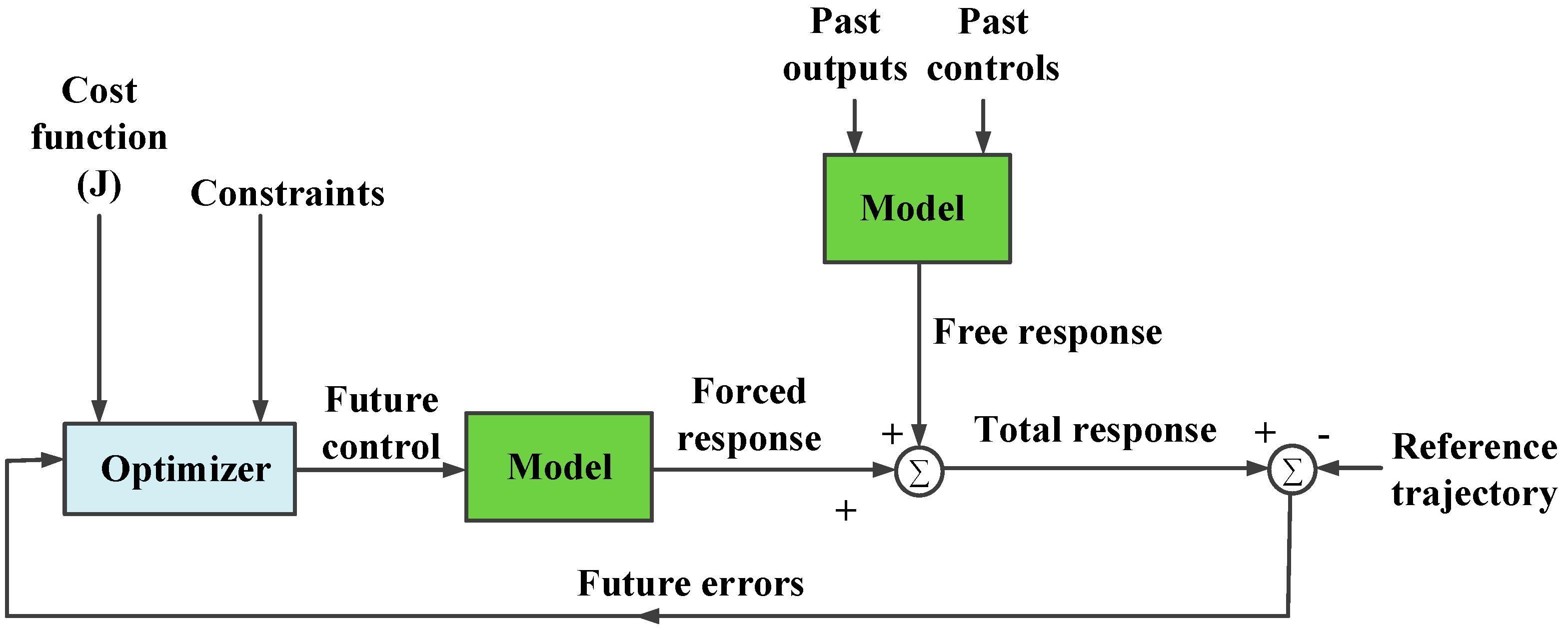
The structure of the applied MPC controller in this study is shown in Figure 5. MPC uses an internal model to predict the future plant outputs based on the past and current values of the inputs and outputs and on the proposed optimal future control actions. The prediction includes two main components known as the free response and the forced response. The free response is the expected behaviour of the output assuming zero future control actions. The forced response is the additional component of the output response due to the candidate set of future controls. In a linear system, the total prediction can be calculated by summing both the free and forced responses; the reference trajectory signal is the target value that the output should attain. The optimizer is used to calculate the best set of future control actions by minimizing a cost function (J), and the optimization is subject to constraints on both manipulated and controlled variables [28].

The main aim of MPC is to minimize the error of predicted output with minimum control effort. In this regard, the objective function is defined as follows:

$$J={\displaystyle \sum _{j=1}^{N_p}{Q}_w}{\left[y(k+j)-r_s(k+j)\right]}^2+{\displaystyle \sum _{j=1}^{Nc}{R}_w}{\left[\Delta u(k+j)\right]}^2$$

(24)

where $N_p \mathrm{and} N_c$ are the prediction and control horizon, respectively. $y(k+j)$ represents the system predicted output at the jth sample; $r_s(k+j)$ is assigned as the future reference trajectory. $Q_w$ and $R_w$ are the positive definite weighting matrices. The first and the second components in Equation (24) are the future output error and the consideration given to the control effort, respectively.

Constraints over the control signal, the outputs, and the control signal changing are as follows:

$$\begin{array}{l}{u}_{\min }=u(k)\le u_{\max }\\ u_{\min }\le \Delta u(k)\le \Delta u_{\max }\\ y_{\min }\le y(k)\le y_{\max }\end{array}$$

(25)

By solving Equation (24) according to the constraints in Equation (25), the optimal sequence of the control signal is given over the horizon N.

5. Simulation Results and Discussions

Simulation results are carried out to validate the efficiency of the proposed MPC for AGC and HPWH. The MATLAB/Simulink software is used for simulations. The proposed controller is applied to AGC and HPWH in a two-area power system. In the considered two-area power system, the areas have the same structure with the same generation units. The rated capacity of each area is 2000 MW, and the nominal load (general loads and HPWHs) of each area is 1840 MW. The base power is considered as 1000 MW in the system. The values of the parameters of the two-area power system are considered in Appendix B. In the design of MPC, the parameters of the MPC controller for both AGC and HPWH in both areas are set as follows: prediction horizon N_p = 20, control horizon N_c = 2, sampling interval = 0.1 s, weights on manipulated variables = 0, weights on manipulated variable rates = 0.1 and weights on the output signals = 1.

In addition, the generation rate constraint is considered for the thermal unit in both areas to be $\left|\stackrel{.}{\Delta P_{thi}} \right|\le 0.1 \mathrm{pu}. \mathrm{MW}/\min =0.0017 \mathrm{pu}. \mathrm{MW}/\mathrm{s}$ and that for the hydro unit in both areas to be $\left|\stackrel{.}{\Delta P_{hydi}} \right|\le 2.7 \mathrm{pu}. \mathrm{MW}/\min =0.045 \mathrm{pu}. \mathrm{MW}/\mathrm{s}$.

Since the secondary frequency control is a dynamic study with a small time frame, it is assumed that the numbers of HPWHs are constant during the simulation. In this study, the rated power consumption of each HPWH is considered 1 kW. It is assumed that 112,000 and 117,000 HPWHs can be controlled in Area 1 and Area 2, respectively. The controllable HPWHs should maintain 90% of their power consumption during their operation to have a contribution to frequency control. The output power and parameters of the aggregated model of HPWH for Areas 1 and 2 are shown in

Table 1. The variation range of the parameters.

Parameters	Area 1	Area 2
Pi: Installed power (MW)	112	117
$T_{AVE}$	2.61	2.66
$T_{SD}$	0.50	0.50

. In the applied model, it is assumed that HPWHs can only participate in frequency control in the range of 90 ± 10% of their rated power consumption in order to maintain the overall efficiency for the customers. This means that the effective capacity of HPWHs to contribute in the secondary frequency control is just ±11.2 MW for Area 1 and ±11.7 MW for Area 2.

Three different scenarios are considered consisting of: step load change, change parameter variations as a sensitivity analysis and a mix of wind farm deviation and random load. In this paper, MPC is applied to AGC and HPWH in a two-area power system simultaneously. The proposed controller is compared with MPC in AGC alone and the optimized proportional-integral-derivative (PID) controller for AGC, which was investigated in [16]. The main aim of the comparison is to demonstrate the effectiveness of HPWH in the secondary frequency control of power system. The root mean square (RMS), peak overshoot, settling time, and peak time of the controllers are also compared.

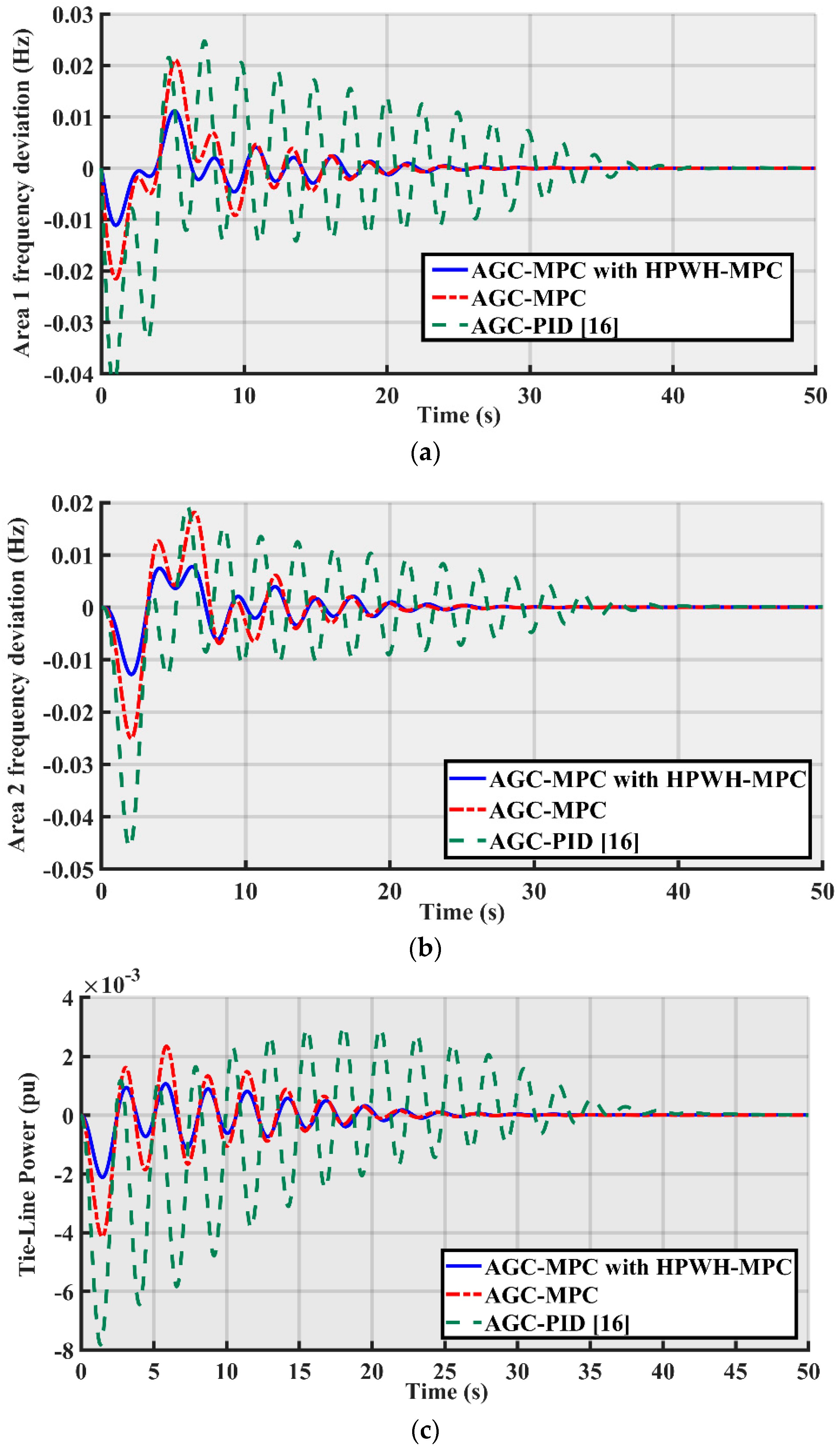
5.1. Step Load Change

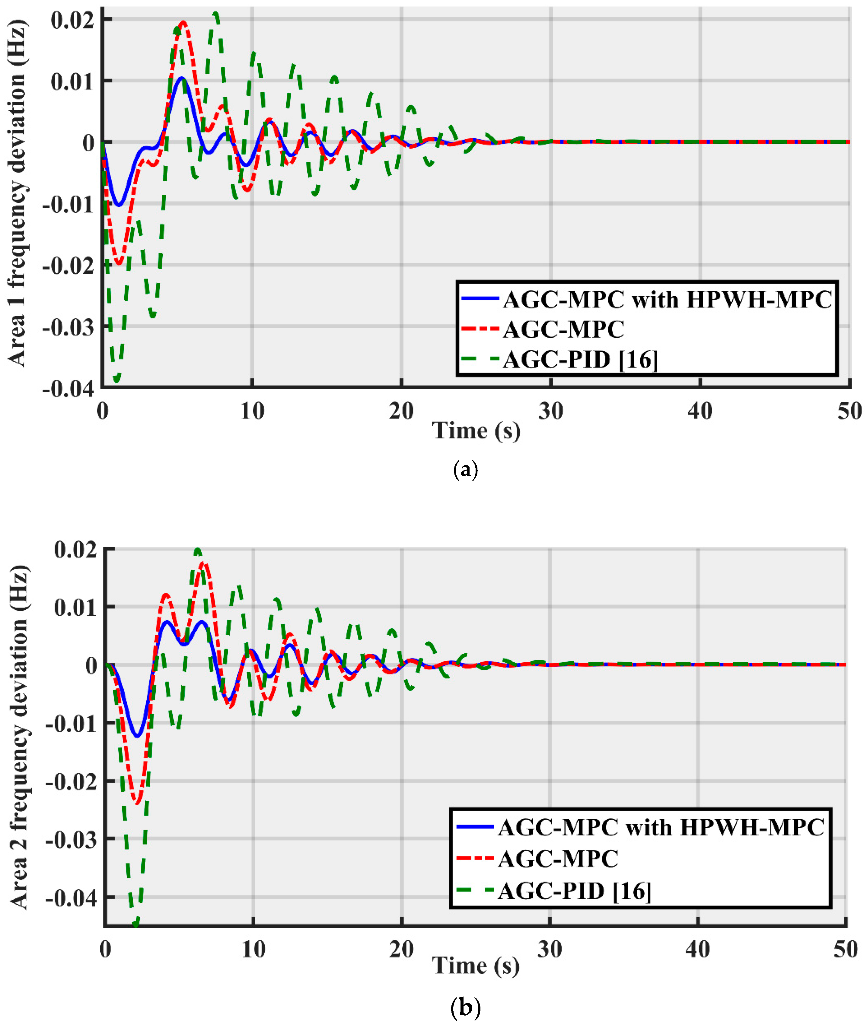
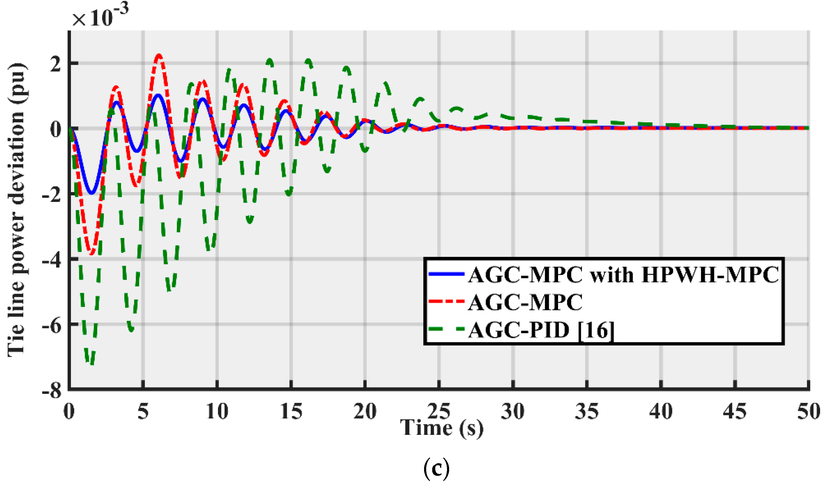
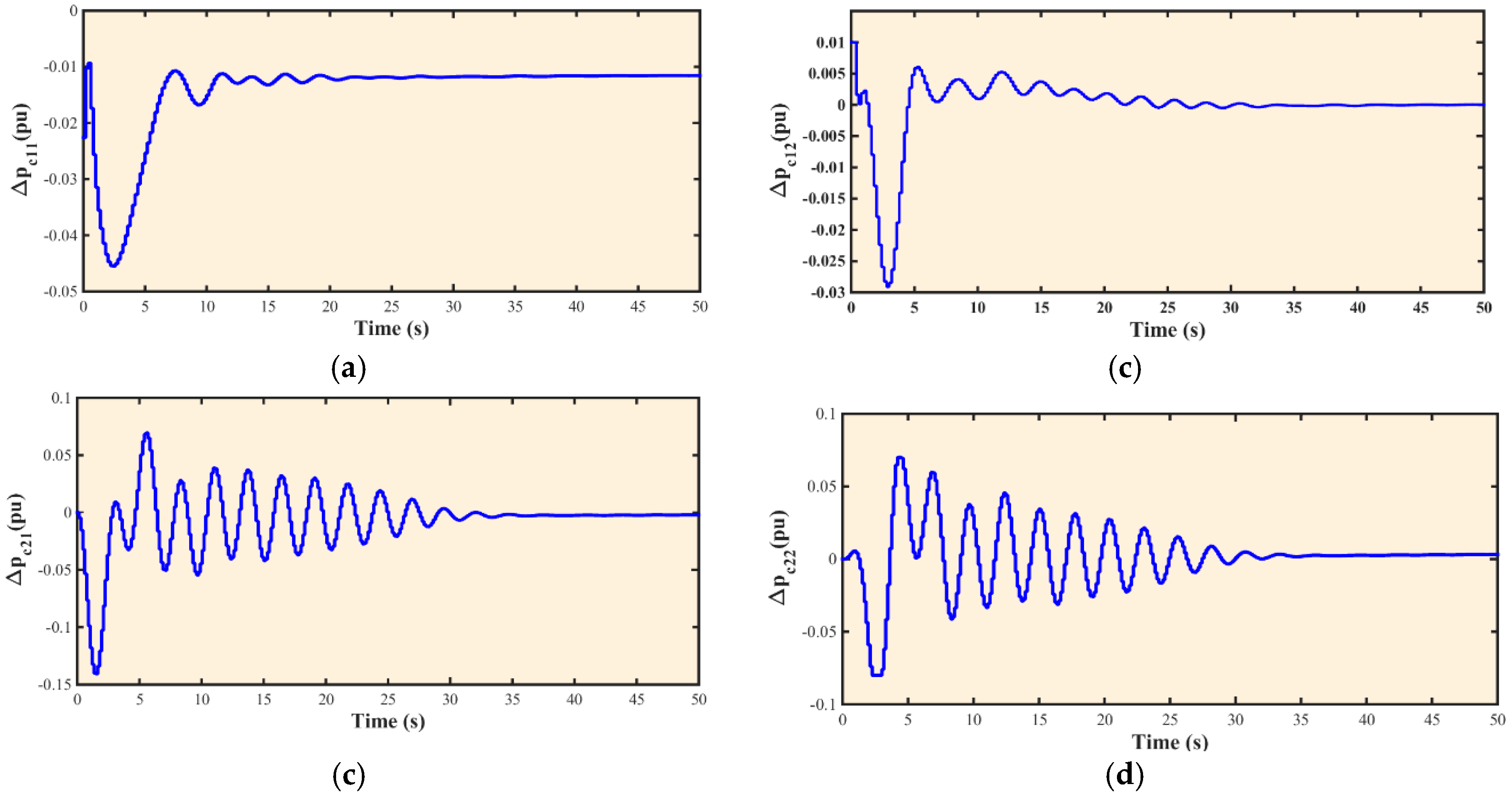
In this scenario, a 0.01 pu (10 MW) step load change is applied in the first area. Figure 6 shows the frequency deviations of Areas 1 and 2 and the tie-line power deviation. MPC controllers have better oscillation damping and settling time over the proposed controller of [16]. Integration of HPWH in the MPC controller results in lower overshoots and better performance than MPC for AGC alone. The control signals of MPC for AGC 1, AGC 2, HPWH 1 and HPWH 2 are demonstrated in Figure 7.

Table 2. Peak overshoot, peak time and settling time for the controllers in the first scenario.

Controller Type	Signal	Peak Overshoot (pu)	Peak Time (s)	Settling Time (s)
AGC-MPC with HPWH-MPC	$\Delta f_1$	−0.0103	2.1560	24.6100
	$\Delta f_2$	−0.0123	2.1560	22.1033
	$\Delta P_{12}$	−0.0020	1.5000	21.0014
AGC-MPC	$\Delta f_1$	−0.0198	1.1000	24.7000
	$\Delta f_2$	−0.0238	2.1539	25.9000
	$\Delta P_{12}$	−0.0038	1.5000	21.1022
AGC-PID	$\Delta f_1$	−0.0390	0.9309	28.1927
	$\Delta f_2$	−0.0449	2.0776	27.1289
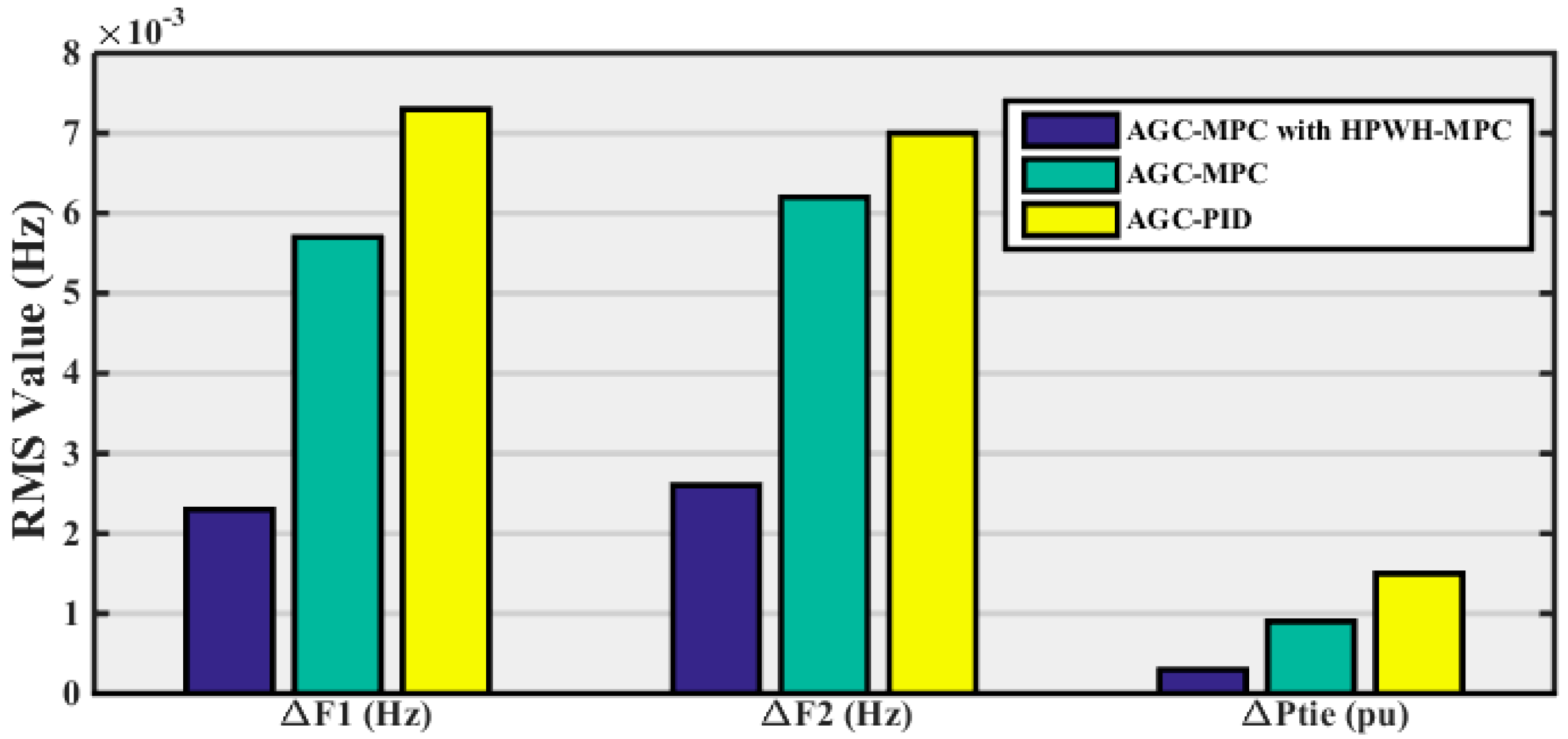
	$\Delta P_{12}$	−0.0074	1.3934	26.5925

presents the peak overshoot in per-unit (pu), peak time in second (s) and settling time in second (s) for the controllers. The peak overshoot for frequency deviation in Area 1 is 0.0103 pu for MPC in AGC-HPWH; and it is −0.0198 for MPC in AGC alone. This means that the peak overshoot is half for the MPC in AGC-HPWH. Same reductions have happened for the frequency deviation in Area 2 and the tie-line power deviation using the MPC for AGC-HPWH. In comparison with [15], the peak overshoots are decreased four-fold by the MPC in AGC-HPWH. 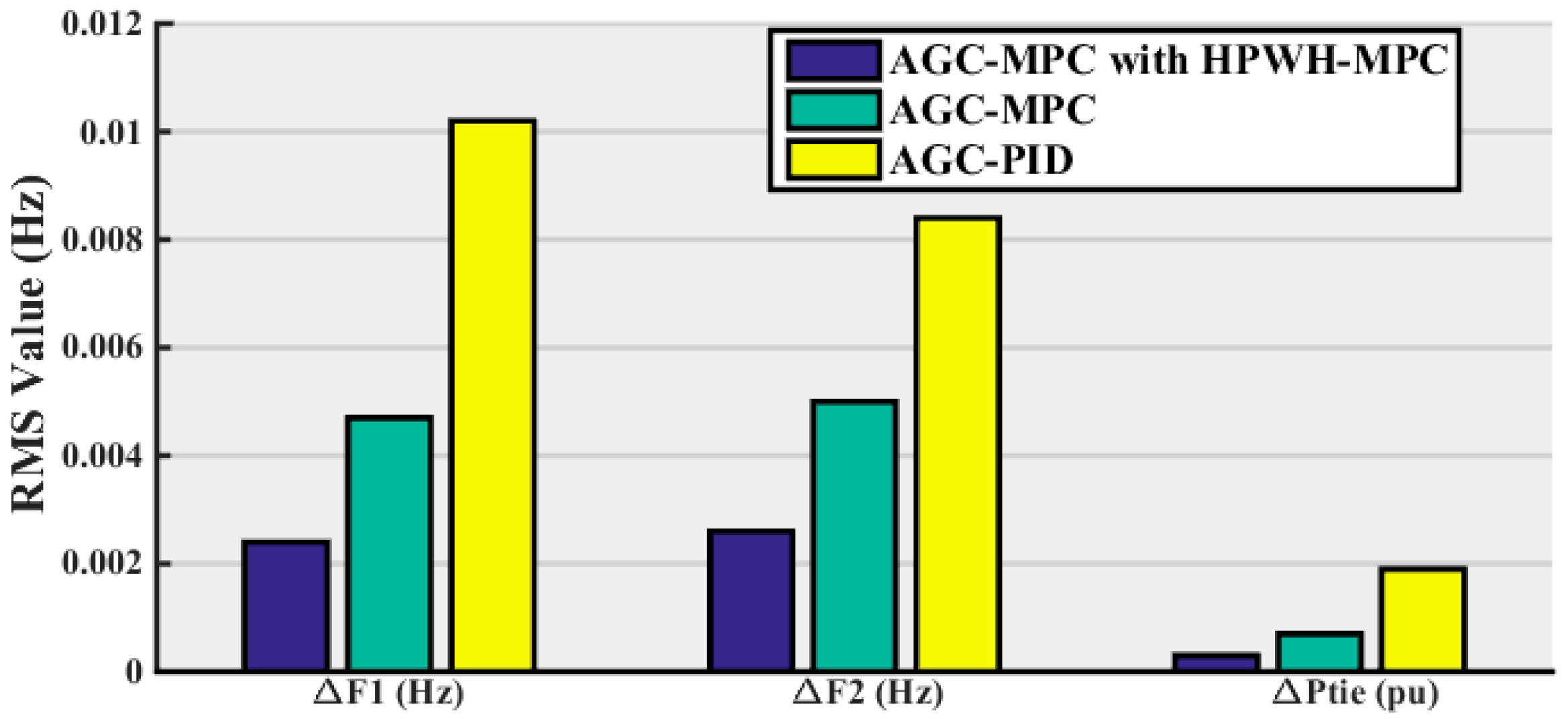Figure 8 demonstrates the RMS value of deviation in hertz (Hz). The MPC in AGC-HPWH has better performance than the other controllers.

5.2. Mix of Wind Farm Deviations and Random Load Change

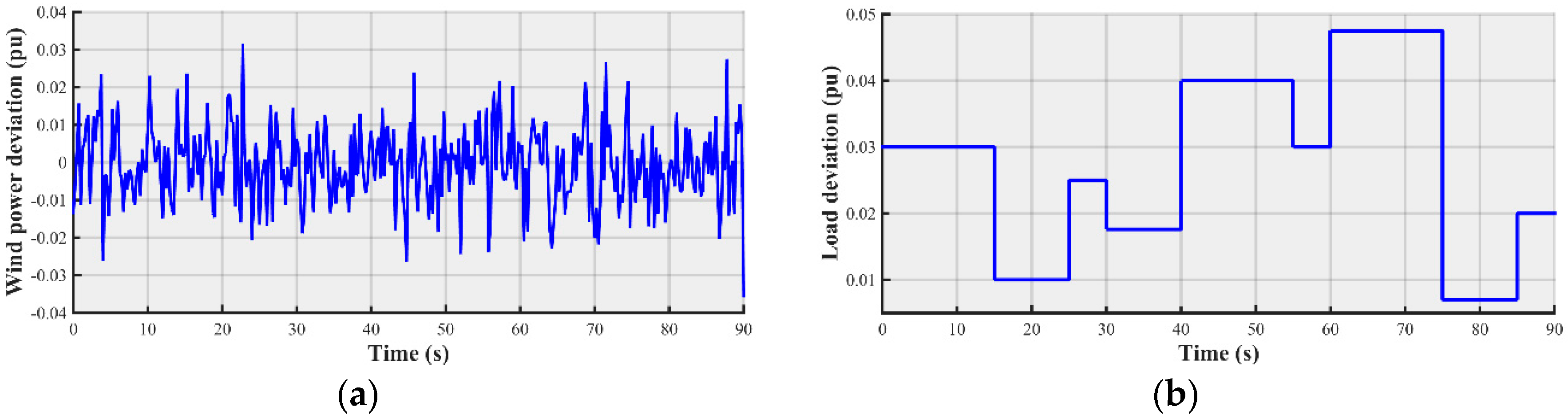
In this scenario, a mix of wind farm power deviation and random load change have been applied to the two-area power system. It is considered that the output power of wind farm has a deviation from a set point. The wind farm output changes between ±0.03 pu from its set point, as demonstrated in Figure 9a. The random load change is illustrated in Figure 9b, which shows deviation between 0 and 0.05 pu. The mix of wind farm power deviation and random load change is used as a real scenario in the power systems.

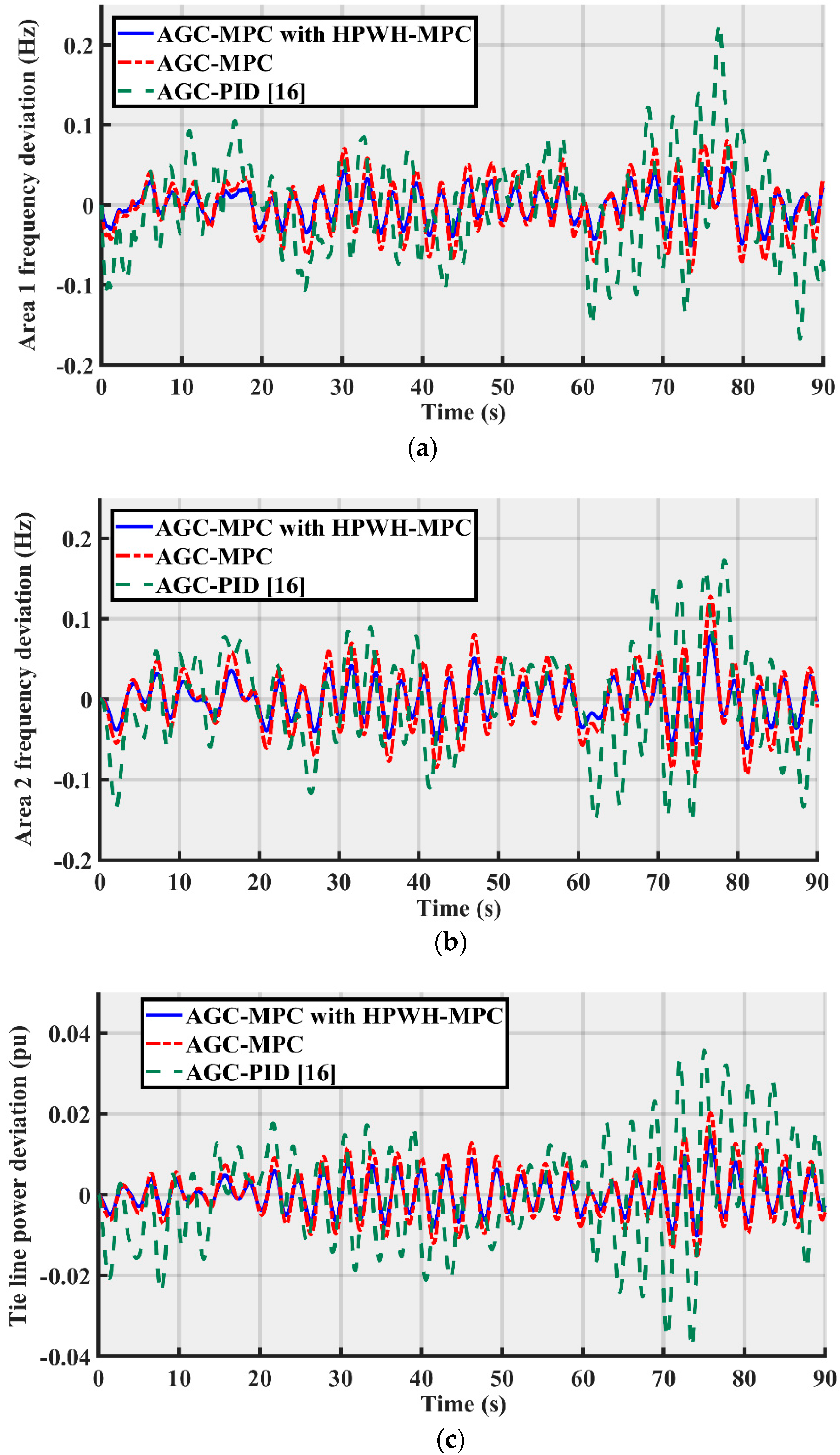
Simulation results including frequency deviations of Areas 1 and 2 and the tie-line power deviation are shown in Figure 10. It has been noticed that with the proposed MPC controller with the participation of HPWH, the system is more stable compared to the system with MPC for AGC alone and the controller applied in [16]. Moreover, the oscillation damping of the proposed MPC is better than the other controllers.

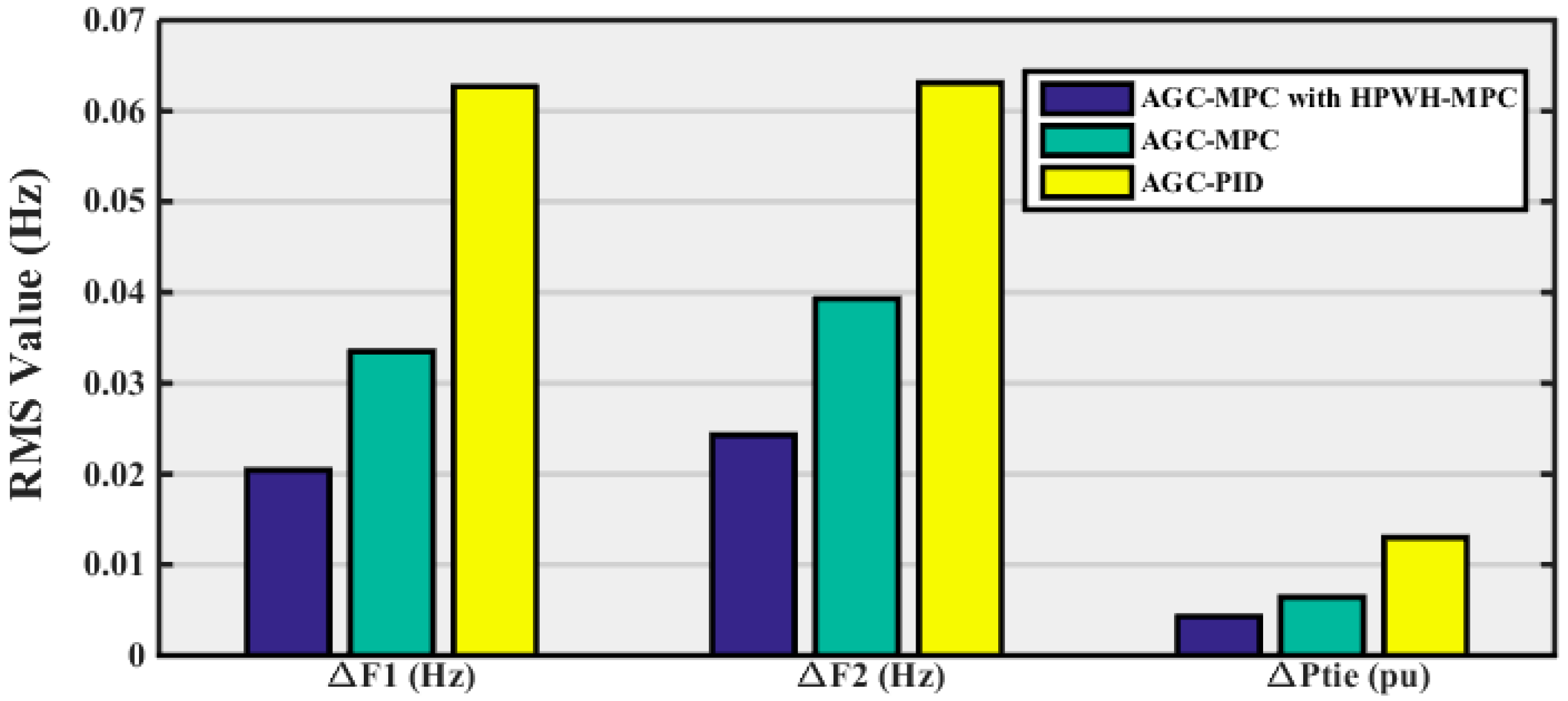
The maximum deviation value and peak time are shown in

Table 3. Peak overshoot, peak time and settling time for the controllers in the second scenario.

Controller Type	Signal	Maximum Deviation (pu)	Peak Time (s)	Settling Time (s)
AGC-MPC with HPWH-MPC	$\Delta f_1$	−0.0507	73.4500	-
	$\Delta f_2$	0.0791	76.5800	-
	$\Delta P_{12}$	0.0139	75.8000	-
AGC-MPC	$\Delta f_1$	−0.0825	73.4500	-
	$\Delta f_2$	0.1281	76.5800	-
	$\Delta P_{12}$	0.0203	75.8000	-
AGC-PID	$\Delta f_1$	0.2257	77.0000	-
	$\Delta f_2$	0.1726	78.3100	-
	$\Delta P_{12}$	−0.0377	73.5000	-

. By integration of the HPWH in the MPC controller, the RMS value of deviation has decreased to 0.0204 pu from 0.0335 pu for the case that MPC was employed for AGC alone. The maximum frequency deviation for Area 1 has a negative value for the MPC controllers. This happens around 73 s of the frequency deviation signal for Area 1. However, the maximum frequency deviation of Area 1 for AGC with the PID controller is 0.2257 pu, and it happens around 77 s. Figure 11 demonstrates a clear comparison between the RMS value of the deviation for the controllers.

5.3. Parameters Variations

The third scenario is a sensitivity analysis to examine the efficiency of the proposed MPC controller for AGC and HPWH. A range of parameters including the governor speed regulation parameter of the gas unit in Area 1 (R_g1), governor time constant of the steam turbine in Area 1 and Area 2 (T_sg1 and T_sg2), power system gain in Area 1 (K_ps1) and compressor time constant in Area 2 (T_cd2) have been changed as shown in

Table 4. The variation range of the parameters.

Parameters	Variation Range
$R_{g1}$	−15%
$T_{sg1}$	+30%
$T_{sg2}$	−20%
$K_{ps1}$	+15%
$T_{cd2}$	−25%

. After changing the parameters in the system, a 0.01-pu step load change has been applied in the first area. Actually, this scenario is an appropriate examination for the robustness of the designed controller.

The frequency deviations and tie-line power deviation are shown in Figure 12 for the parameter variation scenario. The oscillation damping is very slow for AGC with PID controller; while it has improved by MPC in AGC. The proposed MPC for AGC and HPWH has the maximum robustness compared to the other two controllers.

The maximum deviation value, peak time and settling time are shown in

Table 5. Peak overshoot, peak time and settling time for the controllers in the third scenario.

Controller Type	Signal	Maximum Deviation (pu)	Peak Time (s)	Settling Time (s)
AGC-MPC with HPWH-MPC	$\Delta f_1$	−0.0111	1.0000	25.3900
	$\Delta f_2$	−0.0128	2.1000	26.4000
	$\Delta P_{12}$	−0.0021	1.4600	19.5017
AGC-MPC	$\Delta f_1$	−0.0215	1.0000	25.4000
	$\Delta f_2$	−0.0250	2.1000	26.4033
	$\Delta P_{12}$	−0.0041	1.3540	19.6000
AGC-PID	$\Delta f_1$	−0.0424	0.8686	38.1069
	$\Delta f_2$	−0.0460	1.9500	38.1051
	$\Delta P_{12}$	−0.0078	1.3300	35.3305

for the frequency and tie-line deviations after parameter variations. In addition, Figure 13 shows the RMS value of deviation for the three controllers clearly. The proposed MPC for AGC and HPWH has the minimum RMS value of deviation compared to the other two controllers.

6. Conclusions

This paper designed a model predictive control (MPC)-based controller for a two-area power system considering heat pump water heaters (HPWHs) in both areas. The dynamic model of thermal, hydro and gas generation units, as well as the dynamic model of HPWH were employed in the design process. The area control error was used as the input signal to HPWH and AGC to improve the robustness of frequency and tie-line power deviations against the disturbances in different areas. The efficiency of the proposed controller was examined in three different scenarios including: step load change, a mix of intermittent wind farm output and random load change, as well as parameter deviations as the sensitivity analysis. In all scenarios, the performance of the proposed MPC for AGC and HPWH was compared to MPC for AGC alone and AGC with the PID controller. The controllers were compared by the frequency deviations of the areas and tie-line power deviation. The RMS value of deviation showed the superiority of the proposed controller over the other controllers. It was shown that HPWH application in the secondary frequency control of the multi-area power system can improve the frequency and tie-line power performance with an efficient controller.