District Cooling Versus Individual Cooling in Urban Energy Systems: The Impact of District Energy Share in Cities on the Optimal Storage Sizing

Abstract

The energy transition of future urban energy systems is still the subject of an ongoing debate. District energy supply can play an important role in reducing the total socio-economic costs of energy systems and primary energy supply. Although lots of research was done on integrated modelling including district heating, there is a lack of research on integrated energy modelling including district cooling. This paper addressed the latter gap using linear continuous optimization model of the whole energy system, using Singapore for a case study. Results showed that optimal district cooling share was 30% of the total cooling energy demand for both developed scenarios, one that took into account spatial constraints for photovoltaics installation and the other one that did not. In the scenario that took into account existing spatial constraints for installations, optimal capacities of methane and thermal energy storage types were much larger than capacities of grid battery storage, battery storage in vehicles and hydrogen storage. Grid battery storage correlated with photovoltaics capacity installed in the energy system. Furthermore, it was shown that successful representation of long-term storage solutions in urban energy models reduced the total socio-economic costs of the energy system for 4.1%.

1. Introduction

The transition to a low-carbon society got an important impetus following the 21st Conference of Parties, held in Paris in 2015, which resulted in the so-called Paris Agreement. The main long-term goal of the agreement is to keep the increase in the average global temperature preferably to 1.5 °C above the pre-industrial levels [1]. A recent Special Report on Global Warming made by the Intergovernmental Panel on Climate Change reached a conclusion that in order to reach the targets of the Paris Agreement, carbon dioxide (CO₂) emissions will need to fall by 45% until 2030 (compared to 2010 levels), and reach carbon neutrality by the year 2050 [2].

Cities are currently responsible for emitting 70% of the total energy-related CO₂ emissions, while they produce 80% of the world’s gross domestic product (GDP) [3]. Moreover, more than half of the global population lives in cities currently, and it is expected that this share will rise to 66% by 2050 [4]. Due to larger economic activity, more compact spatial layout with higher population densities, cities play an important role in tackling climate problems. Moreover, cities around the world are included in dedicated programs combat climate change such as the Covenant of Mayors for Climate & Energy [5], the Cities Alliance—Cities Without Slums [6], the CIVITAS: Cleaner and better transport in cities [7], the Energy Cities—where action & vision meet [5] and the Climate Alliance [8].

Another important problem, which is more pronounced in urban areas than in rural areas is air pollution [9]. According to the International Energy Agency, 6.5 million premature deaths worldwide can be attributed to the air pollution, placing the air pollution to the 4th place of the largest threats to the health of the humans [10]. For the case of Singapore, it was shown that focusing solely on mitigating climate change emissions, can result in increased air pollution, mainly due to increased biomass use [11].

In a traditional framework of energy systems, the demand for energy is fixed and it needs to be met in all times by different energy sources. The latter framework can become increasingly expensive as more variable renewable energy sources, such as photovoltaics (PV) and wind are introduced, as they cannot be dispatched when needed. In order to reduce both air pollution and climate change related emissions, a shift in the traditional framework started to occur, by creating demand when there is available supply [12]. However, in times when there is very low production from variable renewable energy sources, and demand cannot be reduced enough for the available supply or it is more expensive to reduce it, a resulting difference in demand and supply has to be resolved by different storage solutions.

The first problem detected in the literature was that different energy storage types are rarely represented in the same study, thus making it complicated to detect the interdependency of different storage solutions. Energy storage is often discussed in terms of the power system in general. One review paper focused on the storage solutions for electric vehicles [13]. The authors reached a conclusion that there is still insufficient research carried out about the material support, proper disposal, recycling, safety measures and cost [13]. Another study focused on storage in terms of the integration of wind power [14]. The authors distinguished between the positive impact of storage on power applications, such as voltage and frequency control, as well as on energy applications (storing energy itself) [14]. The authors reached the conclusion that the energy storage can be an effective solution to satisfy the stability and reliability requirements of the power system.

In another set of studies, a focus was placed on the ice storage only. One study examined the system consisting of ice storage, an adsorption chiller and a parabolic trough solar collector [15]. The authors showed that the highest coefficient of performance (COP) in the proposed setup was only 0.15 [15]. In order to increase the performance of the system, some authors suggested the use of double effect absorption chillers in a combination with solar heating plant [16]. The simulated COP of absorption chiller was 1.92, while the measured values showed that the real COP was only 1.21 [16]. Furthermore, much higher inlet temperatures are needed for double-effect absorption chiller compared to the single-effect absorption chiller, which can be problematic for heat sources available at lower temperatures [17]. All those papers pointed to the use of ice storage as daily storage (cooling load shift from day to night), and none of them examined the possibility of using the cold storage in a more seasonal manner.

However, energy storage is a wider concept than just the electrical storage or cold storage. One research paper showed the difference between pumped hydro (electrical), thermal, gas, and liquid storage solutions [18]. The authors concluded that liquid fuel, gas and thermal storage solutions are much cheaper than the electrical storage, as well as that those storage types can store energy for longer periods of time with lower losses [18]. Another paper focused on optimal capacities of different storage types when reaching strict CO₂e emission targets [11]. When looking into minimizing the total socio-economic costs of the energy system, the authors showed that thermal energy storage and hydrogen storage have large potential in future urban energy systems with a high share of electricity generated from PV, while the potential of natural gas and grid battery storage will be much lower [11].

The second problem detected from the literature was a lack of the representation of the long-term storage solutions, usually due to poor (coarse) temporal resolution. A problem that arose in connection with the dawn of the intermittent energy sources, such as wind farms and PV, is the decentralized locations of those energy sources in an energy system. In order to successfully represent and optimize the future capacity investments, energy planning models must successfully represent energy systems both spatially and temporally. In recent reports on long-term energy models, the one from the National Renewable Energy Laboratory (NREL) [19] and the other from the International Renewable Energy Agency (IRENA) [20], it was stated that in order for models to capture both temporal and spatial dimensions, as well as to be computationally tractable, the models use different decomposition techniques or so-called time slicing in order to reduce the complexity of the optimization models. Furthermore, the NREL’s report has clearly stated that the lost ability to represent large-scale storage solutions should be further addressed.

One paper demonstrated the possibility of using statistics-based methods for selecting the optimal subset of the representative days to capture the variability of solar generation and power load in the distribution system [21]. They significantly reduced the number of days that need to be represented, from 365 to 40. However, although they have captured the solar generation and power demand distributions variability, their approach only allows for modelling of intra-day storages.

In Ref [22], the author concluded that for the economic assessment of the energy system it is especially important to capture the value of flexible resources, such as transmission and storage. However, the author has pointed out that the typical models aggregate intra-annual time segments and capacity blocks [22]. The author’s model captured the covariance of resources, operational constraints and regional heterogeneity but energy storage was not able to store seasonal surpluses of renewable energy, according to the author [22].

There are three different papers that tackled the issue of resolution and computational tractability of the energy planning models. The authors in [23] used the National Renewable Energy Laboratory’s Resource Planning Model to demonstrate the difference between results on higher and lower temporal distribution. They simulated different dispatch periods for the “peak-day”, ranging from one day to four consecutive days. They concluded that the shorter simulation periods resulted in over-scheduling of hydro energy and less installation of combined cycle natural gas plants [23]. However, their temporal resolution was still very small (coarse), they focused only on the power sector and no large-scale storages were represented in the model. The same model (Resource Planning Model) was used in another report [24]. The authors carried out a very detailed spatial representation of the distribution and transmission; however, they were still using only consecutive 4-day periods as a temporal resolution. Moreover, the authors explicitly stated that they did not model new storage investments in the model. They reported that increasing sampled dispatch periods had a dramatic effect on computation time, while the investment decisions did not change when changing model configuration from 96-h sample to 24-h sample [24]. The focus of their research was still solely on the power sector, without proper representation of the long-term storages.

To the best knowledge of the authors of this paper, the most detailed research on temporal and spatial trade-offs so far has been carried out in [25]. The authors used the POWER planning model for scenarios with a high share of variable renewable energy generation. The authors concluded that the most trade-offs yield up to the 15% of cost differences. Concerning the spatial resolution, the authors showed that the uniform buildout case resulted in a 10% reduction in cost compared to the site-by-site buildout case. Focusing on the temporal resolution, the authors showed that the total cost is significantly lower with a coarser temporal resolution. However, two limitations, out of the several ones that the authors detected in their paper, are important for this paper. First, the authors reported that their work has focused only on the power sector and it has not captured the current research trend to include all the energy sectors in order to achieve cross-sectoral synergies and second, due to the temporal disjointedness of most days in subsets, the chronological tracking of storages was limited to the 24 h [25].

This paper tackled the both detected problems, the first regarding the optimal storage portfolio depending on the share of district energy supply, and the second, regarding the difference in optimal technology portfolio and corresponding socio-economic costs in energy systems with and without large-scale storage solutions represented. As many different storage solutions exist, it is important to take a holistic look into the energy system, including all of its sectors, in order to be able to track the interplay between different storage solutions. In the existing literature, there is still not enough research carried out on the optimal storage portfolio dependent on different shares of district energy supply. In order to tackle the latter problem, this paper focused on resulting optimal storage portfolio based on the stepwise increase in the share of district energy supply, in this case on district cooling supply for the case of the city of Singapore.

2. Materials and Methods

There are many different energy planning and/or capacity expansion models. The fundamental and the most important difference is between optimization and simulation models. A comprehensive overview of the existing models can be found in [26]. In a recent paper, a critical review has been stated towards the models that report only one optimal solution of the future energy system [27]. The authors claim that the simulation models are better suited for a decision making about the future investments as they typically report several scenarios, i.e. several alternatives, as opposed to the optimization models that typically represent only one (optimal) solution [27]. Although the author of this paper shares the concern about the reporting of the single (optimal) solution to different stakeholders that do not completely understand the complexity of the energy modelling, the number of assumptions and uncertainties about the data, the problem being researched here is especially suitable to be solved by optimization model due to the two reasons. First, the focus of the research is a representation of the different storage solutions, which can be only handled using the optimization techniques. Even the simulation models, such as EnergyPLAN, handle the storage operation via different optimization methods [28]. Second, the geographical scope of this paper is a city scale, as opposed to the more common national or regional models. A city usually has different peculiarities and specifics that need to be taken into account when modelling its energy system. If the focus had been set to the larger geographical areas such as nations, those specifics of a single city would have been averaged out.

Hence, in this paper, a linear continuous optimization model was used to model the representative city of a hot climate. As a linear optimization model, the developed model has many similarities to the more common Balmorel model [29]. The main difference is that the model developed for this specific issue can be more tailored, allowing for better representation of different storage types, as well as different integration technologies such as electrolysers and fuel cells. The results of the model include the optimal operation of the energy system on the hourly resolution, as well as the optimal capacities of different technologies in the energy system. The developed model is specifically tailored for integrated energy modelling, which includes power, cooling/heating, gas, mobility and water desalination sector, including the interactions among those sectors. The goal of the integrated energy modelling is to capture additional efficiencies through integration of different energy sectors, contrary to the models focusing on a single sector only. Thus, although the focus of this paper was on the cooling sector, all the energy sectors were optimized simultaneously in order to capture interactions between different energy sectors.

The full set of equations can be found in Appendix B of this paper, while the most important equations are presented and discussed in this section. Most of the equations were initially developed in [30], and further updated in [11].

The objective function of the model was to minimize the total yearly socio-economic costs of the energy system (Equation (1)). Contrary to the business-economic calculations, the socio-economic costs usually exclude different taxes as those are considered to be internal redistributions within the society. However, the cost of negative externalities such as air pollution and climate change costs can be internalized when calculating the total socio-economic costs. In this paper, the costs of both CO₂e (CO₂, CH₄, N₂O) emissions and air pollutants (NO₂, SO₂, PM) were taken into account. The CH₄ and N₂O emissions were transferred to the equivalent CO₂ emissions using the global warming potential factors. The objective function included levelized investment costs of different technologies, fixed operating and maintenance costs (O&M) and fuel costs. The costs of infrastructure, such as electrical transmission and gas transmission grids were also modelled:

$$\begin{array}{c}\min Z={\sum }_{i=1}^n\left(fix\_O\&M_i+le{v}_{in{v}_i}\right)x_i+{\sum }_{j=1}^m(var\_O\&M_j+\frac{fue{l}_j}{{\eta }_j}+CO2e_j·CO2e_{inte{n}_j}+\\ air\_pol{l}_j·air\_pol{l}_{inten,j})x_j+{\sum }_{k=1}^p\left(gas\_im{p}_k+petr\_im{p}_k\right)x_k[30]\end{array}$$

(1)

Levelized investment costs were calculated using Equation (2). All the infrastructure, including power plants, cogeneration plants, distribution grids and different storage types were annualized and corresponding yearly costs were added to the total yearly socio-economic costs reported in this study:

$$lev\_in{v}_i=in{v}_i·\frac{dis\_rat{e}_i}{1-{\left(1+dis\_rat{e}_i\right)}^{-lifetim{e}_i}}$$

(2)

In total, five different storage solutions were implemented in the model, battery grid storage (Equation (3)), battery storage in vehicles, pit thermal energy storage, hydrogen and natural gas storages:

$$\begin{array}{cc}\hfill battery\_leve{l}_r& =battery\_leve{l}_{r-1}+x_{j,battery,storage\_ch,r}-{\eta }_{batt}{x}_{j,battery,storag{e}_{dis},r}\hfill \\ & -x_{j,battery,storage\_grid\_dis,r}\hfill \end{array}$$

(3)

Storages were modelled using the sets of variables for storage charge, storage discharge and level of energy in the storage. Moreover, storage losses were taken into account. Battery storage of vehicles included another set of variables, the one representing the discharge of electricity to the grid, allowing modelling of the vehicle-to-grid behaviour. All other storage types were modelled in the same manner as the grid battery storage represented by Equation (3).

District cooling balance included district cooling demand that needed to be satisfied, cold generated in absorption chillers, cold from geothermal energy (Equation (4)):

$$ab{s}_{DC}+geotherma{l}_{DC}\ge D{C}_{demand}$$

(4)

while the balance of absorption chillers is given by Equation (5):

$$x_{j,wasteheat,l}+{\eta }_{th}{x}_{j,heat,storage\_dis,r}\ge (ab{s}_{DC}/CO{P}_{abs})$$

(5)

Here it is important to note that the term $x_{j,wasteheat,l}$ represents heat that originates from different sources: gas CHP, waste incineration plant, solar thermal or waste heat from data centres. The waste heat from data centres was assumed to be coupled with heat pumps, which would sufficiently raise the temperature to be fed to single-effect absorption chillers.

A total cooling demand could be satisfied either by district cooling or individual cooling, as presented in Equation (6):

$$D{C}_{demand}+ind\_coo{l}_{demand}\ge coo{l}_{demand,total}$$

(6)

The total individual cooling demand needed to be met by individual chillers is obtained using Equation (7). Individual chillers were assumed to be building level air conditioners:

$$chille{r}_{individual}\ge ind\_coo{l}_{demand}$$

(7)

The remaining part of the model developed in this paper, which was used for representing the other sectors of the energy system, can be found in Appendix B.

The model was built using the Matlab interface and Gurobi optimization solver. Optimizations were carried out on a personal computer, with an i7 processor (1.9 GHz), 16 GB of physical RAM, and 25 GB of virtual RAM, dedicated from 500GB SSD hard disc. A single optimization run took 30 min in the most time-consuming run.

3. Case Study

Singapore was chosen for the case study as it is a 100% urbanized country, at a high level of economic development and suitable for district cooling research as it is located very close to the equator. Being a country—city, a large agglomeration with lots of available data, Singapore represents very well the urban zones of many developed countries, especially those with a similar climate.

Singapore is one of the most densely populated cities in the world, with 7900 people per km². It is a very developed region, having the 3rd largest GDP at power purchase parity (PPP), with 93,905 USD per capita according to the World Bank [31]. Large population and high economic activity result in a large energy use per capita. According to the International Energy Agency, Singapore’s primary energy demand per capita was 53.8 MWh in 2015 [32]. Singapore is the most developed part of south-east Asia and thus, its energy consumption is already high [33]. Currently, south-east Asia is rapidly developing, both in terms of population and economic activity. Consequently, it can be expected that the neighbouring cities will see a significant increase in primary energy demand to meet the needs of its increasing population. For the case of Malaysia, the IEA forecasts increase in energy demand by a factor of 2 until the year 2040 [33].

Hence, the results implemented for this case study are transferable to other cities located in the warm regions, as it can be expected that most of the cities that are now significantly increasing economic activity will see much higher energy demand for cooling purposes in the future.

Different assumptions were made as a part of this research. CO₂e emissions factors, capacities of energy facilities, energy demand and the description of the transportation sector can be found in great detail in [34] and [35]. The energy supply of Singapore is dominated by gas power only plants, as can be seen in

Table 1. The energy supply of Singapore in the reference scenario.

Plant Type	Capacity [MW]	Fuel	Efficiency	Reference
Power plants	2225	Natural gas/LNG	47.5%	[36,37]
Waste-to-energy plants	256.8	Waste	16.7%	[36,37,38]
PV	33.1	-	12.4% (capacity factor)	[36,38]

.

The following technologies were predefined in the optimization model: solar heating, absorption chillers, waste heat from data centres coupled with heat pumps to reach sufficient temperatures [39], PTES storage and geothermal energy in district cooling sector; grid battery storage, waste and gas combined heat and power plants, wind turbine, PVs and vehicle-to-grid in the power sector; natural gas transmission grid (import), hydrogen storage, gas storage, solid-oxide electrolysers and fuel cells, syngas to natural gas and syngas to gasoline syntheses and gasoline import in gas and mobility sectors. Finally, other technologies included in the model were individual chillers (individual cooling) and reverse osmosis for desalination of seawater. It is important to notice that all of those technologies were predefined in all the scenarios of this research paper. However, based on the conditions in a specific scenario, different optimal set-ups were possible in different scenarios.

As the focus of this paper was on the optimal portfolio of different storage types depending on different shares of district cooling and individual cooling, it is important to discuss different assumptions regarding the implemented storage types. In this paper, individual cooling included cooling solutions from an apartment level up to the one whole building. To be counted as district cooling, at least two buildings had to be connected to the district cooling grid.

Pit thermal energy storage (PTES) was assumed for district cooling purposes. It is used to store large quantities of warm water before it is fed to single effect absorption chillers. There are two main reasons why pit thermal energy storage was chosen for district cooling sector instead of ice (cold) storage. First, the current literature review shows that no cold storage is currently being used as seasonal storage, while there are plenty of real-world installations of pit thermal energy storage solutions [40]. Second, for ice storage charging, very low temperatures are needed, which cannot be obtained by water-lithium bromide absorption chillers. Instead, the ammonia-water solution should be used. However, the ammonia-water solution was reported to have a lower coefficient of performance than the water-lithium bromide solution [40].

A single-effect water-lithium bromide absorption chiller technology was adopted for this study, in order to make it possible to utilize as much waste heat from different sources as possible. The coefficient of performance (COP) of 0.7 was used. District cooling system was organized as a centralized system, as both PTES and absorption chillers were centrally located. On the other hand, building level air conditioners, designated in this research paper as individual cooling, had a COP of 4.0.

The cost of the district cooling distribution grid with water as a medium flowing through the pipes was adopted from [34], and the price of 37 €/MWh of yearly delivered cold energy was used. The losses of district cooling grid are significantly lower than the district heating grid. One reason is a lower temperature difference between the water flowing through the pipes and the surrounding ground, and the other is a generally larger diameter of distribution pipes in the case of the cooling grid, resulting in a lower area-to-volume ratio and corresponding heat losses. For the tropical region, average losses of 4.8% were reported [34], which is also the number used in this study.

Hydrogen was assumed to be stored in a cavern type of storage at 50 bars. Methane storage was also assumed to be an underground cavern. Grid batteries and vehicle batteries technology were lithium nickel cobalt aluminum oxide (Li-ion) NCA. Assumed investment costs and efficiencies can be seen in

Table 2. Investment costs and efficiency of different storage solutions.

	Investment Cost (€/MWh)	Efficiency *	Reference
PTES	540	75%	[41]
Methane storage	99	97%	[41]
Hydrogen storage	11,000	96%	[41]
Grid battery	127,300	91%	[42]
Vehicle batteries	127,300	91%	[42]
** vehicle to grid mode		79% **	[43,44]

* including charging losses, ** including direct current to alternating current transformation

.

In this paper, a detailed assessment of the potential CO₂ source for natural gas synthesis was out of the scope of the paper. However, the National Climate Change Secretariat of Singapore estimated that large amounts of CO₂ could be extracted from industry and gas power plants in their Carbon Capture and Utilisation roadmap [45]. It is important to keep in mind that CO₂ capture would increase the reported costs of the energy system, which was excluded from this study.

Availability of space for installing large amounts of low-density energy generators, such as PV, is often an issue in highly populated cities in south-east Asia. Singapore has a particularly high density of population, with many competing uses of available space. Regulations for using available space are very tight, and hence, the available area for PV installations has to be constrained. According to the solar photovoltaic roadmap developed for Singapore, the maximum available space for PV installations corresponds to 12,250 MW of peak capacity [46]. The referenced PV capacity already included expected development of the efficiency of PV panels that will consequently require less area for the same capacity than it is the case today. The latter includes also 20% of available seawater where floating PV could be installed. In order to take into account the PV capacity constraint, two different scenarios were developed; the first included the constrained PV capacity (dubbed PV constrained scenario) and the second did not include the constraint on PV capacity (dubbed unconstrained PV scenario). The latter would mean that Singapore should import one part of the energy generated from PV from nearby regions.

Out of other technologies, solar thermal was constrained to 2000 MW also due to space constraints, while geothermal was constrained to 50 MW_e, in line with the current estimates for geothermal potential [47]. Finally, waste heat from data centres was constrained to 735 MW_th, a conservative estimate taken from [35].

4. Results

Several different optimization runs were carried out in order to reach two major conclusions. The first was to detect the difference between the optimal configuration of the energy system with and without the large-scale energy storages, in order to evaluate the potential error when reducing the time resolution in the capacity extension models. This part of the research included spatial constraints influencing maximum PV and solar thermal capacity, as described in the Case study section.

The second gap detected in the literature review was the difference in optimal capacities of different technologies based on different shares of district cooling and individual cooling. In order to reach conclusions on this issue, optimizations were run stepwise (in steps of 10%), starting from 0% of district cooling (100% of individual cooling) to 100% of district cooling (0% of individual cooling). Two scenarios, in this case, PV constrained and unconstrained PV, were run in order to assess the difference between transition the energy system to an isolated one and non-isolated one.

One can note from

Table 3. Results of the comparison of energy models with and without large-scale storage representation (Storages represented optimization run and Storages not represented run had all the predefined technologies the same, except that storage capacities were constrained to zero in the case of Storages not represented scenario).

	Storages Represented	Storages Not Represented	Difference
Total socio-economic costs [mil €]:	8012	7685	−4.1%
Capital costs [mil €]:	3773	3464	−8.2%
Operating costs [mil €]:	3609	3592	−0.5%
CO2e costs [mil €]:	607	607	−0.1%
CO2 costs [mil €]:	605	605	−0.1%
Air pollution costs [mil €]:	23	22	−3.9%
NOx emissions [kg]	11,751,113	11,711,620	−0.3%
SOx emissions [kg]	0	0	-
PM emissions [kg]	19,694	19,627	−0.3%
CO2e emissions [Mt]:	29	29	−0.1%
Primary energy demand (incl. Industry) [GWh]	163,871	163,914	0.0%
Methane consumption [GWh]	73,258	73,021	−0.3%
Oil consumption [GWh]	41	7	−81.8%
Renewable [GWh]	17,662	17,801	0.8%
Waste consumption [GWh]	5989	6166	2.9%
Industry consumption–natural gas [GWh]	66,920	66,920	0.0%

. that total socio-economic costs were 4.1% lower when different storage solutions were included in the urban energy modelling. This difference shows that it is important to be able to represent different storage solutions in energy planning of future urban energy systems. The latter difference would have been even larger if spatial constraints influencing the maximum installed PV and solar thermal capacities had been relaxed. The main difference in costs occurred from capital savings in gas infrastructure, as gas storage replaced one part of gas CHP plant capacity and one part of the gas import capacity.

The differences in the optimal configuration of the energy system can be seen in

Table 4. The difference in the optimal energy system configuration with and without representation of large scale storages. Only non-zero capacities are presented (including all the storages). Optimal capacities were the one that resulted in the lowest socio-economic costs, for valid conditions in each of the specific scenarios.

Capacities [MW]	Storages Not Represented	Storages Represented
solar heating	2000	2000
Electric chillers	43	0
Absorption chillers	4780	6074
PTES storage (GWh)	0	417
battery storage (GWh)	0	4
waste CHP	170	170
gas CHP	5929	4785
PVs	12,250	12,250
gas net import	13,950	10,960
Hydrogen storage (GWh)	0	0
gas storage (GWh)	0	112
SOEC	0	0
SOFC	0	0
gasoline import	813	459
electric vehicles battery capacity (GWh)	15	16 *
Reverse osmosis	31,620	34,937
Geothermal DC capacity	50	50
DC capacity	4607	6074
Non DC capacity	9727	9517

* No vehicle-to-grid mode in non-storage optimization run.

. One can notice from Table 2 that although different storage solutions resulted in a reduced socio-economic cost in the case of storages represented scenario, CO₂ emissions were almost the same. The reason is that the lower share of district cold generation via absorption chillers was replaced by individual electric chillers, which had a high COP value of 4. However, the large share of individual cooling resulted in higher total socio-economic costs.

By comparing Table 3 and Table 4, one can notice that the increased flexibility via the different storage representation in the energy system model resulted in significantly lower total socio-economic costs, which mainly originated from the lower capital costs.

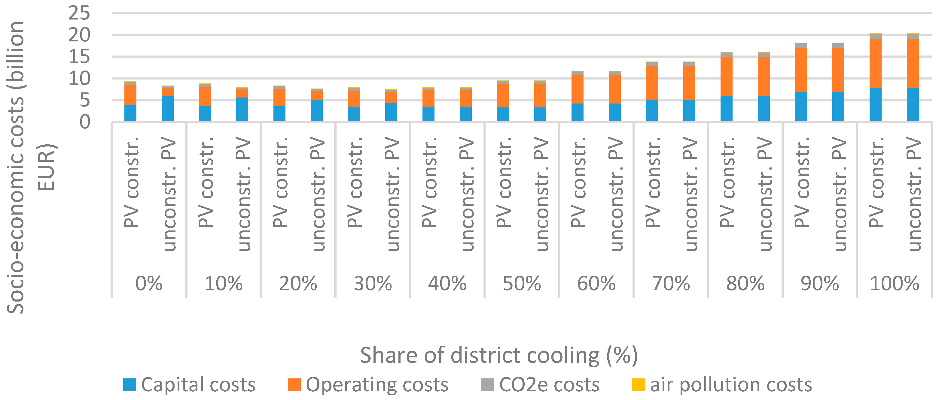
Results of the stepwise increase in the share of district cooling can be looked at in Figure 1, Figure 2 and Figure 3. The difference in socio-economic costs for different shares of district cooling and individual cooling, for both PV constrained and unconstrained PV scenarios, can be seen in Figure 1. The lowest socio-economic costs occurred at 30% penetration of district cooling in both cases. For the PV constrained scenario, the socio-economic cost at 30% share of district cooling was 7.9 billion EUR, while for unconstrained PV scenario the total socio-economic cost was 7.5 billion EUR. Thus, the corresponding difference of allowing larger capacities of PV resulted in a cost reduction of 5.1%, all other assumptions being the same. Increasing the share of district cooling from 50% to 100% resulted in significantly higher total socio-economic costs of the energy system.

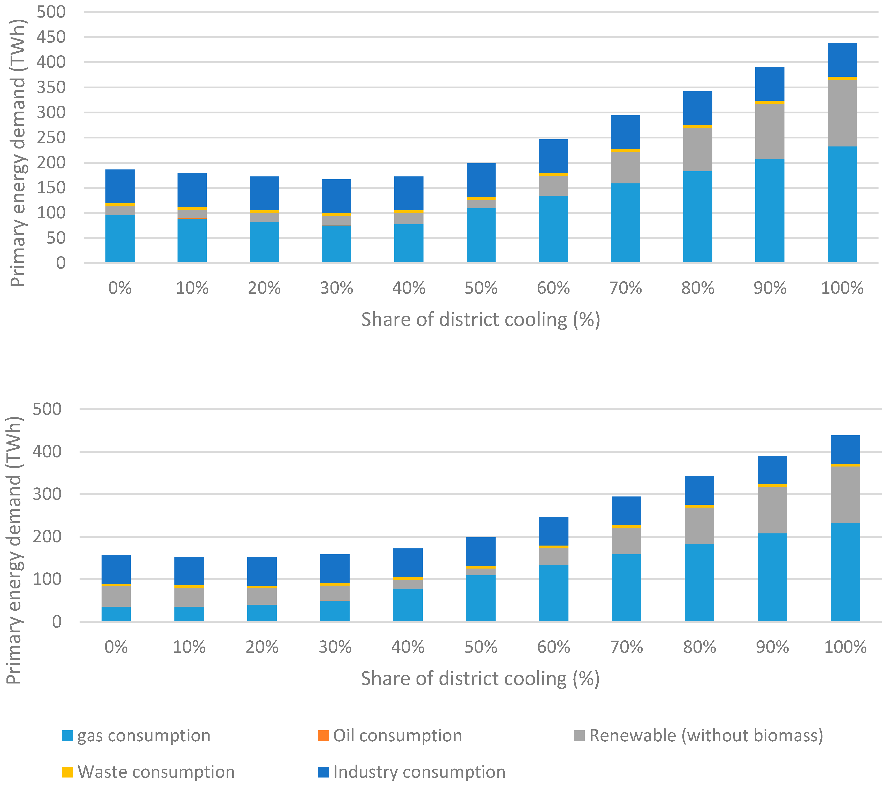
Total primary energy demand in PV constrained and unconstrained PV scenarios can be seen in Figure 2. Primary energy demand started to increase significantly after surpassing the share of district cooling of 50%. At lower shares of district cooling, unconstrained PV scenario had generally lower primary energy demand. On the other hand, at higher shares of district cooling, primary energy demand in PV constrained scenario was lower than in the unconstrained PV scenario. Starting from the district cooling share of 40%, optimal capacities and corresponding costs were the same in both PV constrained and unconstrained PV scenarios. The reason is that the optimal capacity of PV in all those runs was lower than the PV capacity constraint in PV constrained scenario.

The total socio-economic costs were reducing until the share of district cooling of 30% was reached in both scenarios. The main reasons were better utilization of waste heat from gas CHPs and waste incineration plants, which was utilized for a cold generation in absorption chillers, as well as utilization of PTES, a cheaper storage option than the battery storage. Starting from the district cooling share of 40%, socio-economic costs of the energy system started increasing again. The main cause for the latter behaviour was a lack of low-cost waste or excess heat. Without enough heat available, gas CHP needed to consume more fuel in order to generate a sufficient amount of heat needed for absorption chillers. Having more waste heat available could result in a higher optimal share of district cooling than in this case study.

PV constrained scenario had generally a lower share of capital costs and a larger share of operating costs than in the unconstrained PV scenario. The main reason is that the unconstrained PV scenario had significantly larger capacities of PV and grid batteries, resulting in higher upfront investment and lower running costs.

Both air pollution and CO₂e costs were generally higher in PV constrained scenario than in the unconstrained PV scenario. The lowest CO₂e emissions and air pollutant emissions were in the unconstrained PV scenario, without any district cooling. The reason for the latter is that a significant capacity of PV did not cause any carbon emissions or air pollution, while gas CHP plant that was dominating energy source for larger shares of district cooling contributed to both carbon emissions, as well as air pollution.

Optimal shares of different storage capacities can be seen in Figure 3. The largest capacities were those of methane and PTES storage types. Generally, demand for grid battery storage is low in different cases, as smart charging and vehicle-to-grid technology are already providing lots of flexibility in the energy system. The only exception is the case of unconstrained PV scenario, up to the share of district cooling of 30%. In those cases, the grid battery storage capacity was relatively large, as was the capacity of PV. The latter points to the conclusion that grid battery storage can be an economically viable solution if they can be utilized for many day-night charging and discharging cycles, as it was the case when large capacity of PV existed in the energy system. Discharge of electricity for the grid in the vehicle-to-grid mode was maximally utilized in the unconstrained PV scenario, at 30% share of district cooling, with the discharge of electricity from vehicle batteries equalling 0.72% of the total electricity generation over the year. The lowest socio-economic costs in both scenarios occurred at 30% share of district cooling.

At 30% of district cooling share in PV constrained scenario, optimal storage capacities of PTES, grid battery, methane, hydrogen and electric vehicle batteries were 2.7 GWh, 3.9 GWh, 195.1 GWh, 0 GWh and 15.6 GWh. In the case of unconstrained PV scenario, optimal storage capacities of PTES, grid battery, methane, hydrogen and electric vehicle batteries were 5.34 GWh, 28.3 GWh, 0 GWh, 0 GWh and 20.3 GWh. The behaviour of optimal PV capacities and battery storage capacities showed a correlation between those two technologies. Capacities of all the technologies for all the optimization runs can be found in Appendix A.

5. Discussion

Focusing on the first detected issue that was addressed in this paper, looking into Table 3. One can notice significant savings in total socio-economic costs of the energy system that were achieved only by better representing different storage solutions. In that sense, this paper is directly addressing a research gap detected in recent NREL’s [19] and IRENA’s [20] reports on energy modelling. The main difference for the case of Singapore is more efficient utilization of gas infrastructure. The difference in total socio-economic costs in systems with and without different storage solutions represented would have been even larger if PV capacity had been left unconstrained. A sensitivity analysis was carried out with unconstrained PV capacity in order to check the latter claim. It was found out that the difference in total socio-economic costs of the energy system was 7.9% when different storage solutions were represented. The main difference originated from the optimal capacity of PV, which was 52% larger in the case when storage solutions were successfully represented.

Moreover, one can observe in Table 3 a significant difference in oil consumption in the two cases, however, it should be noted that oil consumption in both cases is very low compared to the current oil consumption of Singapore. The reason for almost no oil consumption is that industrial oil consumption was switched to natural gas consumption and most of the transport sector was electrified, a result of the optimization model used in this research paper.

Focusing on the second issue addressed in this paper, looking into primary energy demand in Figure 2, one can note that at high shares of district cooling, primary energy demand tend to rise significantly. There are two main reasons for significantly higher primary energy demand in cases with a higher share of district cooling. First, at lower shares of district cooling, there is a large capacity of individual air conditioners (building level air conditioners), with a coefficient of performance of 4. Hence, ambient thermal energy that was used in the cooling cycle was not accounted for as primary energy demand. The second reason is that large shares of district cooling consequently had a large demand for natural gas. After all the low-cost heat sources were utilized, further heat generation from gas CHPs was not the optimal procedure in energy efficiency terms. Introduction of SOEC and SOFC in some of the runs with a higher share of district cooling resulted in additional conversion steps, increasing the losses in the energy system.

The optimal share of district cooling in both PV constrained and unconstrained PV scenarios was 30%. As the current share of district cooling in Singapore is very low, reaching the share of 30% could be challenging. One option would be to connect very densely populated central parts of the city, which includes mostly commercial buildings, to the district cooling and gradually spread the system towards residential areas. The other option would be first to implement district cooling in areas that are currently being developed, and connect the other buildings to the district cooling grid when major retrofit of buildings is scheduled, the approach proposed in [34].

It is important to discuss here the sensitivity of the results. During the case study representation, it became clear that Singapore is significantly lacking in resources for very large shares of renewable energy in the total energy consumption. Singapore is a city with a large energy demand per capita, and it is a very densely populated city. Moreover, it does not have a good wind potential for either onshore nor for offshore turbines. Due to the lack of available space, PV plants built on the ground are not an option in the current urban development plans of Singapore. All of these reasons contribute to the optimal share of district cooling of 30%. The amount of low priced waste heat is a very sensitive parameter, significantly influencing the results. Cities with similar climate, but higher amounts of waste heat availability, would probably result in a significantly larger optimal share of district cooling.

Larger shares of district cooling caused a higher need for waste heat that could be utilized via absorption chillers. To match that additional demand, optimal capacities of gas CHPs were larger than in the case of higher shares of individual cooling. The latter was also matched with much higher capacities of methane storage compared to other storage types. When maximum PV capacity was unconstrained, battery storage capacities were larger than in the case of PV constrained scenario. The reason for the latter is that battery grid storage and vehicle batteries in the form of smart charging were used by the system as day-night storage solutions, while methane, hydrogen and PTES storages solutions were used by the system for much longer periods.

Generally larger capacities of gas and thermal energy storage compared to the grid battery storage confirmed the finding from [18]. Somewhat contrary to the [18], in this paper, optimal grid battery capacities were found to be also rather large, especially in the case of unconstrained PV scenario. The latter can be contributed to the specific weather patterns of Singapore, having no clear distinctions between different seasons and only day-night distinctive insolation pattern (without seasonality effect). In the future work, the optimal capacities of grid battery storage should be assessed in a different setup in order to detect its correlation to different variable renewable energy sources; however, with larger optimal capacities of wind energy compared to PV.

Some regions like the Caribbean have a high potential of both wind and solar energy and thus, large penetration of cost-efficient renewable energy technology can be achieved without large district energy supply systems [48]. On the other hand, this case showed that for the case of Singapore, that has large potential only for solar energy and not for wind energy, a 30% share of district cooling was optimal.

Although there are not many research papers dealing with an optimal share of district versus individual cooling taking holistic energy modelling approach, there is a lot of research on the optimal share of district heating. Energy roadmap Europe has found that optimal shares of district heating versus individual heating solutions would be 66% for Italy and Spain, 50% for the Netherlands and Germany, and between 27% and 43% for most other EU countries [49]. The reason for the difference between the larger optimal shares of district heating compared to district cooling can be explained by climate specifics. Warmer regions that have very high cooling density demands usually correlate with high global insolation, having a large potential for solar energy development. Consequently, a combination of solar energy and efficient heat pumps can be more cost-effective than having very large shares of district cooling based on waste heat utilization in absorption chillers. To check the optimal share of district cooling versus individual cooling, future research projects could encompass different cities across the world, using a similar model to the one developed for this study.

6. Conclusions

Two detected research gaps were part of this study. In order to assess the optimal share of district cooling versus individual cooling taking holistic energy modelling into account, several optimization runs were carried out with a stepwise increase in district cooling share. It was shown that optimal district cooling share for the case of Singapore was 30% in both scenarios that were carried out; one with constrained PV capacity that reflected spatial constraints, and the second with unconstrained PV capacity that would include the use of nearby space, outside of the city borders.

In order to improve the research on the second detected research gap, two cases were assessed, one with five different storage types represented, and the second one without long-term storage types represented. The results revealed that an error by not representing storage technologies in energy planning models was 4.1% for the case of Singapore. The latter difference raised to 7.9% when PV capacity constraint was relaxed.