Object-Oriented Usability Indices for Multi-Objective Demand Side Management Using Teaching-Learning Based Optimization

Abstract

This paper proposes Object-Oriented Usability Indices (OOUI) for multi-objective Demand Side Management (DSM). These indices quantify the achievements of multi-objective DSM in a power network. DSM can be considered as a method adopted by utilities to shed some load during peak load hours. Usually, there are service contracts, and the curtailments or dimming of load are automatically done by service providers based on contract provisions. This paper formulates three indices, namely peak power shaving, renewable energy integration, and an overall usability index. The first two indices indicate the amount of peak load shaving and integration of renewable energy, while the third one combines the impact of both indices and quantifies the overall benefit achieved through DSM. The application of the proposed indices is presented through simulation performed in a grid-tied microgrid environment for a multi-objective DSM formulation. The adopted microgrid structure consists of three units of diesel generators and two renewable energy sources. Simulation has been done using MATLAB software. Teaching-Learning-Based Optimization (TLBO) is adopted as the optimization tool due to its simplicity and independency of algorithm-specific control parameters. Five different cases of renewable energy availability with results validate the efficiency of the proposed approach. The results indicate the usefulness in determining the suitable condition regarding DSM application.

1. Introduction

1.1. Motivation

DSM can be considered as the coordinated reduction in load during a specific time so as to maximize the energy usage from renewable energy and minimize the generation cost. Most of the research on DSM have tried to explore the technical benefit of DSM in design and operation area, recently some studies have tried to quantify the economic benefits of DSM. Thus motivation of the work is to quantify both the technical and economic benefits of DSM using OOUI.

1.2. Literature Review

Currently, the power industry is facing numerous challenges because of the fast-changing structure of the power network. The integration of small-size renewable energy sources with the conventional grid has become a significant challenge. In addition to this, the uncertainty of power availability from these renewable energy sources is also a serious concern. The search for a suitable scheme which provides a solution for technical and commercial challenges associated with the above-discussed problems is the main area of research for system operators. DSM has appeared as a potential solution for many of these problems.

Any scheme that involves alteration in operation of a complex system should be reliable to a certain level. A reliability study of a power system with DSM is presented in [1]. Since a plan for load curtailment can only be prepared when load forecasting is reliable, stochastic optimization and Gray Wolf Optimization (GWO)-based load forecasting and subsequent DSM programs are presented in [2,3]. Load shifting is also an alternative method of performing DSM. In this aspect, a corrective load shifting program is found to be a better option to conventional preventive load shifting [4,5]. In another work, loads are categorized in rigid and flexible types, and DSM is performed keeping in mind the adaptability of the flexible loads [6]. A novel application of DSM to smoothing the peaks of load curve in a small demand area in the Sultanate of Oman is described in [7]. The key contribution was load profile prediction based upon which the DSM program was prepared. The DSM program developed here handles the issue of variable power generation from solar energy-based generation. In a work, the uncertainty due to wind power generation and its impact on the DSM scheme has been discussed [8]. The methodology discusses the fulfillment of two key objectives of DSM, i.e., minimization of emission and cost. Battery storage and diesel-based energy sources are also employed with solar or wind generators to improve the reliability of the system. A DSM program for the hybrid photovoltaic system has been also proposed in the literature [9]. The target of DSM was set to minimize the system component size and extension of battery life. This indicates that the system operation and its reliability can also be improved through DSM.

A unique presentation of DSM using a spatial and temporal approach has been proposed in [10]. Spatial and temporal DSM is a mathematical improvement carried over the conventional DSM mathematical system. In this improved scheme, a power diagram for each load bus is prepared to accomplish the optimality for a complete system. With the proposed DSM method, the overall performance of the system increases with reduced operating cost and increased voltage quality. A Genetic algorithm (GA)-based DSM program has been presented in [11]. With accurate prediction, the DSM program presented successfully improves the economic dispatch. The impact of solar and wind energy variability has been depicted through sensitivity, and its impact on the DSM program has been analyzed [12]. An optimal sizing problem has been investigated with and without DSM, and a solution with DSM employed was found to be more suitable while sizing the sources for optimal operation [13].

In some of the recent works, DSM has been explored for energy management of the microgrid structure as well. The energy planning and management can be done in a certain advance time duration. This duration may be one day (day ahead scheduling), one hour (hour ahead scheduling), or it can be real-time management (real-time scheduling). In one recent work, demand response-based hierarchical energy management of a microgrid was proposed using a scenario-based optimization scheme [14]. In an hourly scheduling study, it was found that the payment for community aggregated electricity consumption can also be reduced through optimal hourly scheduling of electrical loads [15]. Following the same line, work has also been carried out for consumption management. The electrical appliances can be scheduled for optimal consumption. An informatics solution has been proposed for optimal scheduling which interacts with different appliances and utilities and coordinates the optimal scheduling of loads [16]. In a microgrid, multiple sources operate simultaneously. An operation algorithm has recently been proposed for proper scheduling of individual sources. The algorithm is based on the interaction between different sources and operates a demand response for energy management [17]. The load reduction or load profile flattening has also been done based on a shifting optimization algorithm. This method successfully lowers the electricity consumption and bill payment [18].

A prominent challenge for a demand response program is the probabilistic nature of renewable sources. The conventional numerical methods to optimize the system often fail to reach the best possible solution. Adaptive schemes like genetic algorithm- and artificial intelligence-based optimization have been tried upon to obtain the best possible solution in such adverse mathematical environment. A DSM program based on the artificial immune network has been proposed for the peak load problem [19]. Results show that the adaptive technique enabled the DSM program to keep the peak load within one percent of the desired limit. The Artificial Neural Network (ANN)-based decision-making system has also been proposed in the literature to manage the energy storage system and solar PV-based generator to reduce the consumer electricity cost [20]. The adaptive techniques have not only improved the stress issue and design aspect, but also helped in obtaining better economic performance through DSM. Using the load problem of the individual customer, the appliance usage is so adjusted that a minimum bill for each consumer is obtained [21].

To implement the DSM program, an optimization technique is required as a tool for problem-solving. There are conventional techniques used to solve the DSM problem in the literature, such as linear programming [22,23] and dynamic programming [24], which give a globally optimal solution. However, with an increase in the size and complexity of the problem the solution search space increases. These approaches required more computational effort and time with the addition of more variables and variety of constraints. To resolve this problem, modern approaches, such as simulated annealing and GA, have been proposed as alternatives [25,26].

The evolutionary techniques are advanced optimization schemes where the optimization problem is solved with the help of specific control parameters. For example, GA uses the mutation rate and crossover rate, and particle swarm optimization uses the inertia weight, and social and cognitive parameters. In all these evolutionary methods, the tuning of parameters has a significant effect over the end result. The TLBO algorithm has an advantage over other methods in this aspect. It need only the fewer parameters, thus reducing the burden of tuning the parameters. Thus, the TLBO algorithm is simple and effective [27,28,29]. Due to these advantages, TLBO has been adopted in this work.

All works discussed here so far have tried to explore the technical benefit of DSM in design and operation areas. However, there are very few works available in the literature where an attempt has been made to quantify the economic benefit of DSM. An index-based assessment of DSM program is discussed in the literature to quantify the technical and economic benefits that can be obtained through the application of DSM. A DSM quality index quantifies the technical gain, whereas a DSM appreciation index quantizes the economic benefits of DSM program [30]. The work quantifies the benefits of DSM. However, the index includes only a single outcome, i.e., load current reduction, and is based only on per unit energy cost reduction. The other advantages of DSM, such as greater integration of renewable energy sources and peak load shaving, are not included in the index calculation. Therefore, need arises for the quantification of DSM usability which includes the desired objects of DSM. This paper proposes an OOUI which can be used for deciding the usability of the DSM program for a certain application.

1.3. Contribution and Paper Organization

Major contributions of this work are as follows: (1) This work proposes three indices, namely, peak power shaving index, renewable energy integration index and an overall usability index; (2) the proposed indices help the operator determine conditions during which DSM is relatively more beneficial in term of peak power shaving and renewable energy integration; (3) the economic benefit of demand response can also be quantified using the proposed index mechanism; and (4) OOUI can provide aid to the system operator in policy-related decisions.

The rest of this paper is organized as: Section 2 presents the mathematical modeling of the system under study. Section 3 presents a microgrid-DSM formulation. Section 4 introduces the proposed indices and their analysis. Section 5 presents the TLBO-based optimization scheme and its adaption for the demand response program. Section 6 presents the case studies based on MATLAB simulation, results, and discussion. Section 7 provides the conclusion of the proposed research work, followed by the references.

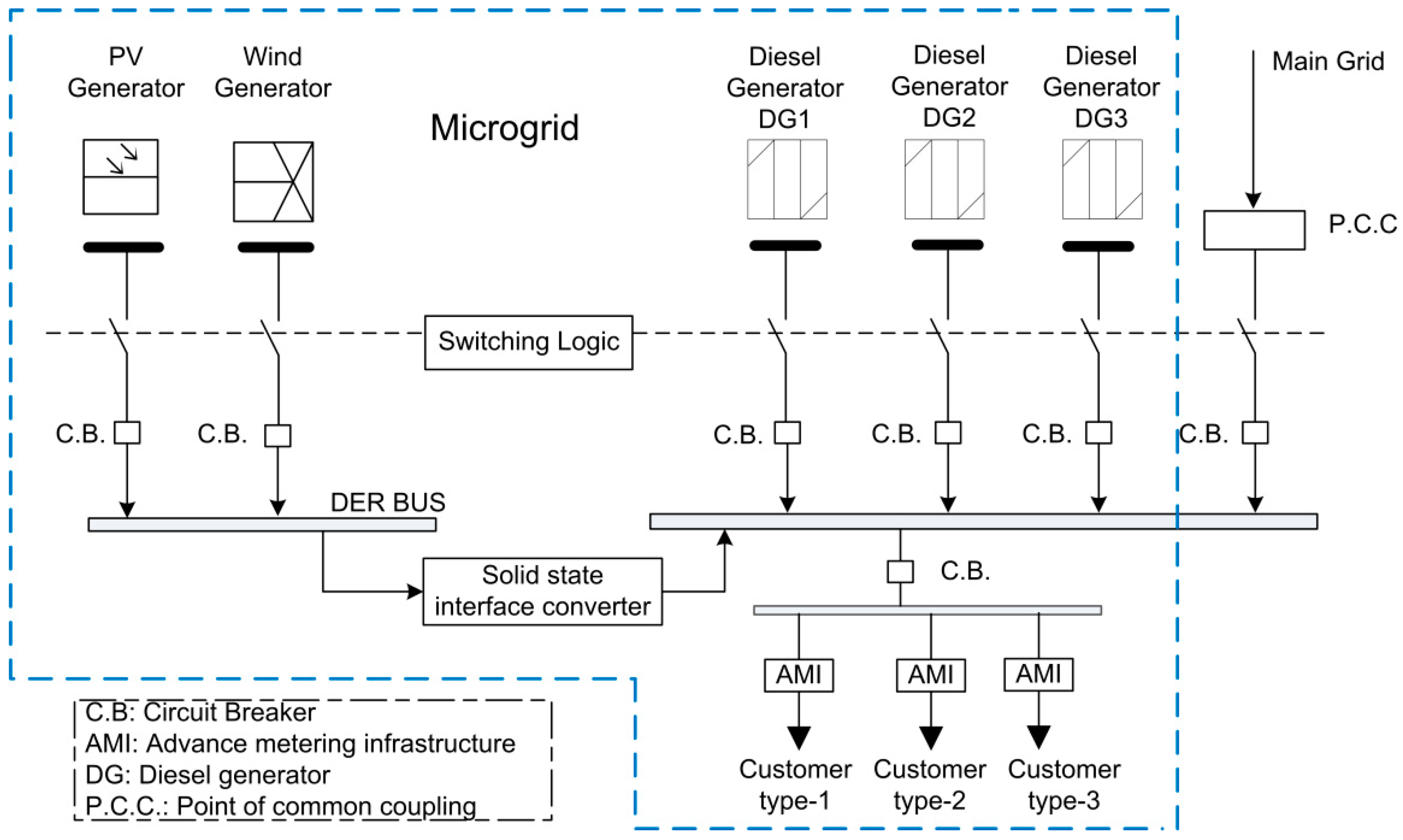
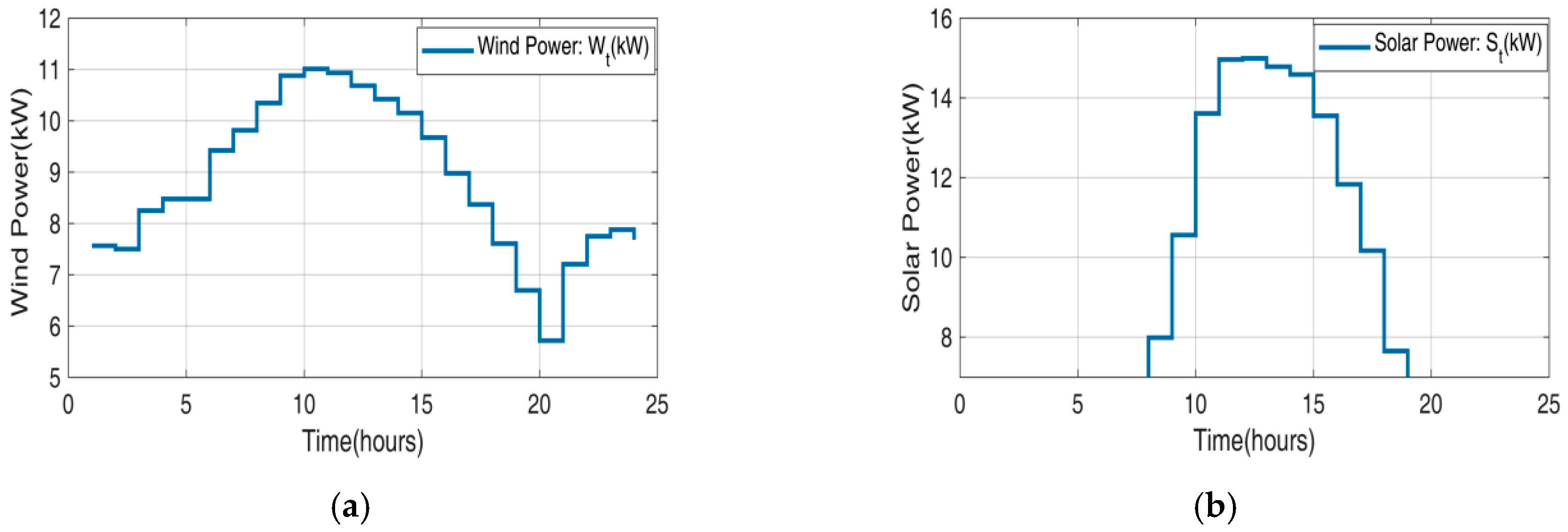
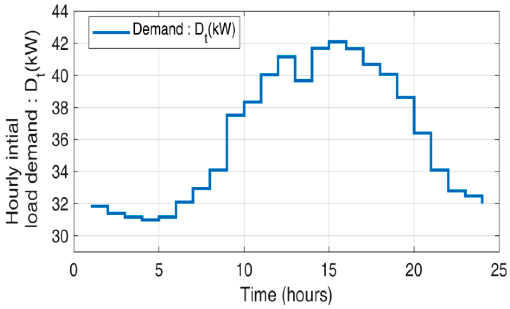
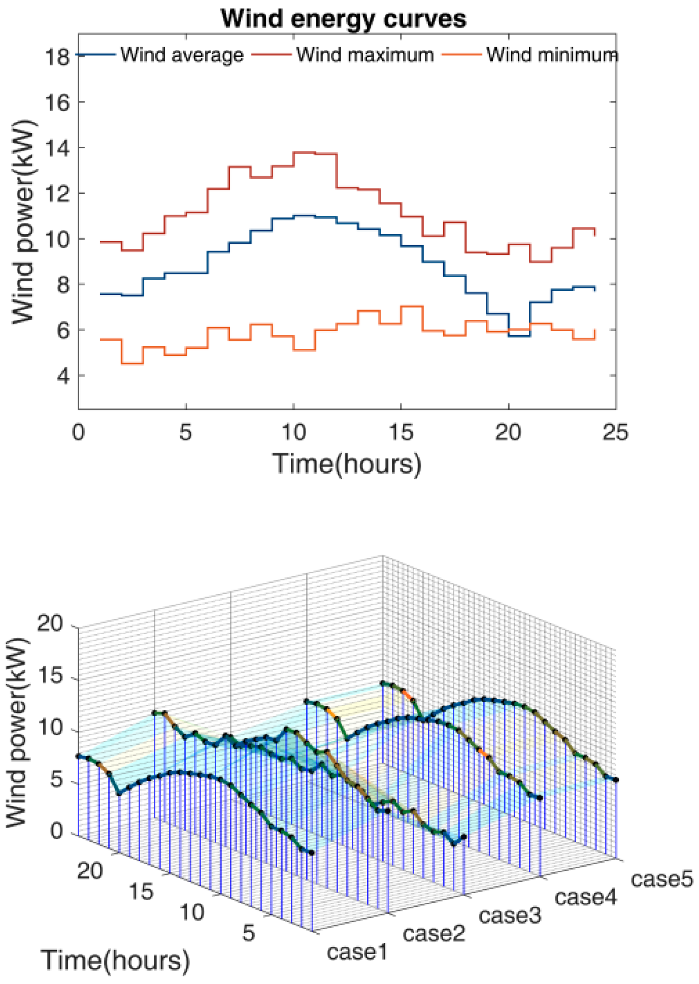
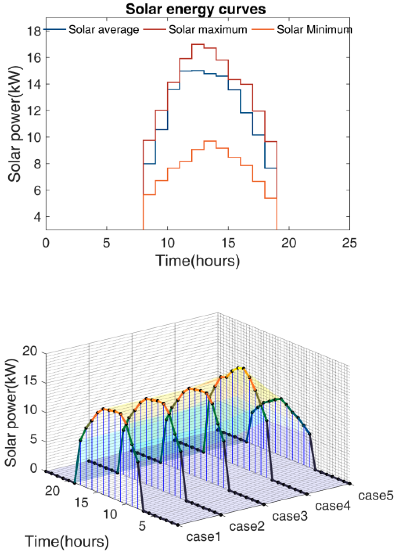
2. Microgrid Modeling

The schematic diagram of the microgrid is given in Figure 1. This microgrid consists of three units of diesel generators (DG1, DG2, DG3) and two renewable energy sources: one wind and one solar generator. The switching logic block in Figure 1 takes care of scheduling all six energy resources. Three different types of customer are assumed to be connected in this system using advanced metering infrastructure (AMI). AMI provides all the required information of the customer load to the utility. A scheduling interval of 24 h is used in this paper. Renewable energy sources are coupled with DGs and the main grid through a solid state interface converter which allows power flow from the grid and distributed energy resources (diesel, wind, solar energy resources) to loads connected at the point of common coupling. The maximum interchangeable power allowed between the main grid and microgrid is 4 kW.

Figure 2a,b presents the availability of electrical energy from wind- and solar-based power plants in our microgrid system from Figure 1. Figure 3 shows the initial hourly demand of three customers. Figure 4 shows the hourly power interruptibility cost$({\lambda }_{j,t}$) in dollars. Descriptions of the dieselgeneration fuel cost function with its parameters are as follow:

$$C_l\left(P_{l,t}\right)=a_l{P}_{l,t}^2+b_l{P}_{l,t}$$

(1)

where $P_{l,t}$ is the power output and $a_l,b_l$, are the fuel cost coefficients related to the lth DG at any time instant t; for example, if the cost function of DG2 is $C_2\left(P_{2,t}\right)$ = $a_2{P}_{2,5}^2+b_2{P}_{2,5}$ then here $a_2$ and $b_2$ are parameters related to DG2 and $P_{2,5}$ is the output power of DG2 during the 5th hour. Information about the conventional DG parameters are tabulated in

Table 1. Data for diesel generator cost parameters.

Parameter	Abbreviations	$\mathbf{D}\mathbf{G}1$	$\mathbf{D}\mathbf{G}2$	$\mathbf{D}\mathbf{G}3$
First fuel cost coefficient $\left(\$/\mathrm{kW}\right)$	$a_l$	0.06	0.03	0.04
Second fuel cost coefficient ($/kW)	$b_l$	0.5	0.25	0.3
Minimum output power limit (kW)	$P_{l,min}$	0	0	0
Maximum output power limit (kW)	$P_{l,max}$	4	6	9
Ramp up rate(kW/hour)	$D{R}_l$	3	5	8
Ramp down rate(kW/hour)	$U{R}_l$	3	5	8

, providing all the cost parameter data of the diesel generators.

The solar and wind modeling presented here is based on a complex and detailed model. For the detailed model please referred to [12,31].

Wind energy conversion units develop electrical energy from wind speed using the mathematical relation of Equation (1a), referred to in [12,31]:

$$E_t=0.5\eta {\rho }_{air}{C}_{p}A{V}^3$$

(1a)

where η is the efficiency of the wind generator, A is the swept area of the wind turbine rotor; V is the velocity of the wind at the hub height, $C_p$ is the power coefficient of the wind turbine, and $\rho$ is the air density.

The PV generator output per hour is given below [12,31]:

$$E_{pv}=\eta A_c{I}_{pvt}$$

(1b)

where η is the efficiency of the solar $pv$ generator, $A_c$ is the area of the solar $pv$ array, and $I_{pvt}$ is the per hour incident of solar irradiation (kWh/${\mathrm{m}}^2$) on the solar array.

Load modeling is an important part of the demand response program as the main target of the program is to reschedule the consumer loads. The loads in this paper are taken as aggregate loads as individual customers. Unlike some other load modeling where loads are presented in terms of individual load types (i.e., air conditioners, refrigerators, etc.), or presented as characteristic impedance equations (i.e., constant impedance loads, non-linear loads, etc.), this paper considers loads as cumulative consumer units. The flexibility of the load is presented through a term ${\theta }_i$ which indicates the willingness of individual customers to participate in the rescheduling process. The willingness value varies from 0 to 1, which indicates zero percent willingness to one-hundred percent willingness. The details of customer-related parameters are discussed in Section 3.2 and tabulated in

Table 2. Customer cost function related data.

Description	Abbr.	Customer Type1	Customer Type2	Customer Type3
Customer type	$i$	1	2	3
1st coefficient related to customer cost function	$K_{1,i}$	1.079	1.378	1.847
2nd coefficient related to customer cost function	$K_{2,i}$	1.32	1.63	1.64
User Type	${\theta }_i$	0	0.45	0.9
Curtail limit $\left(\mathrm{kW}\right)$	$C{M}_i$	80	85	90

.

The microgrid conceptually utilizes the potential of solar and wind energy generation units. The small-scale generation units based on renewable energy sources are normally interfaced into the conventional grid at the low-voltage distribution level. Such microgrid structures lower the cost, negating traditional economies [32]. The studied system adopted in this paper is a microgrid structure in grid-tied mode. The adopted microgrid structure consists of a solar-based generator, wind-based generator, and three conventional diesel generators at the source end.

The mathematical model describing the structure and behavior of individual components and the complete system is prepared and presented in the next sections.

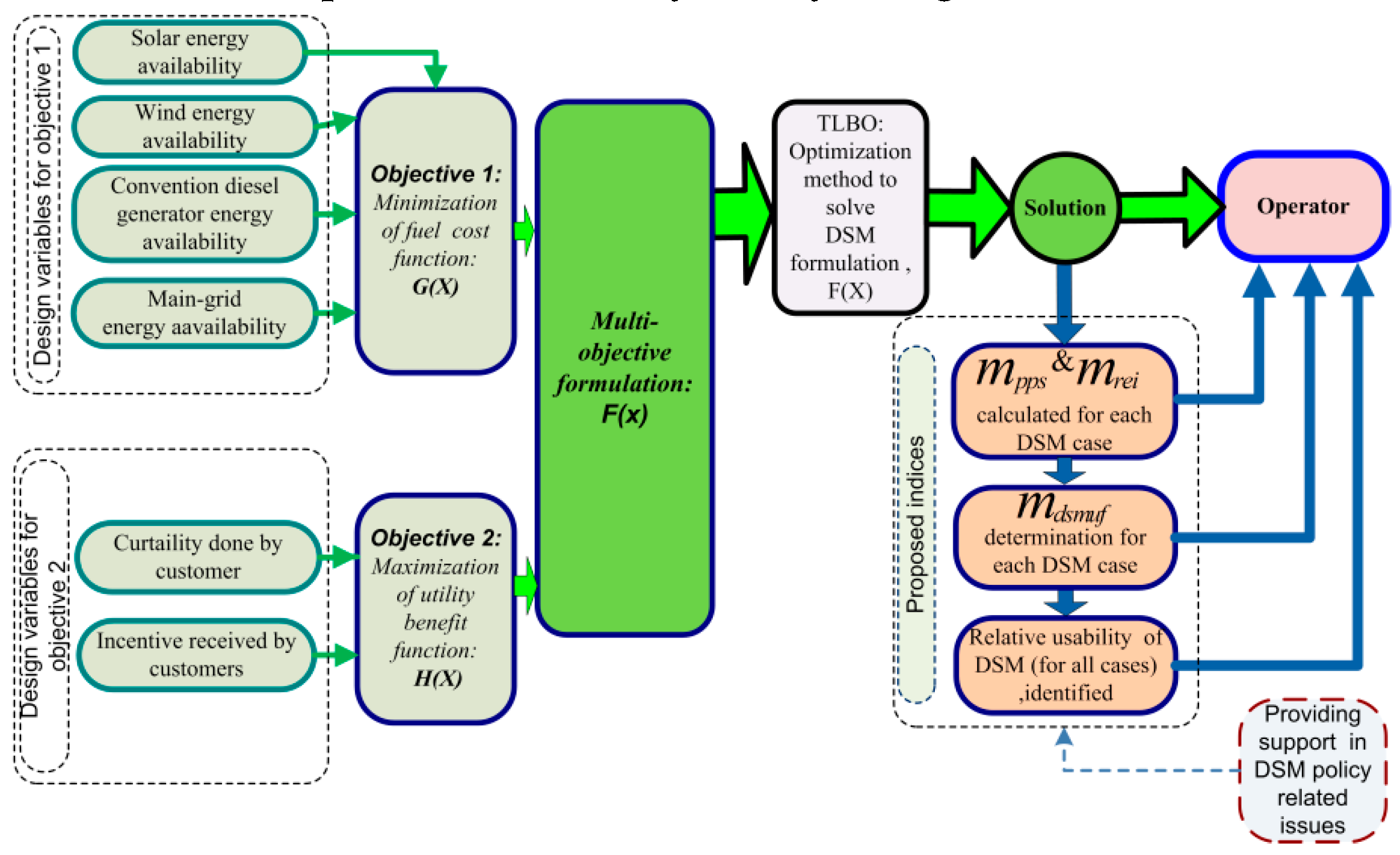
3. Microgrid DSM Problem Formulation

This section presents the microgrid-DSM formulation. Optimization results of this formulation are used in the upcoming section to show the application and usability of the proposed indices.

Adopted microgrid DSM problem formulation has two objectives, namely, minimization of fuel cost function G(X) for diesel generators by maximum utilization of renewable energy sources, and maximization of utility benefit function using DSM. The formulation of the multi-objective function involves these two objectives, as shown in Figure 5.

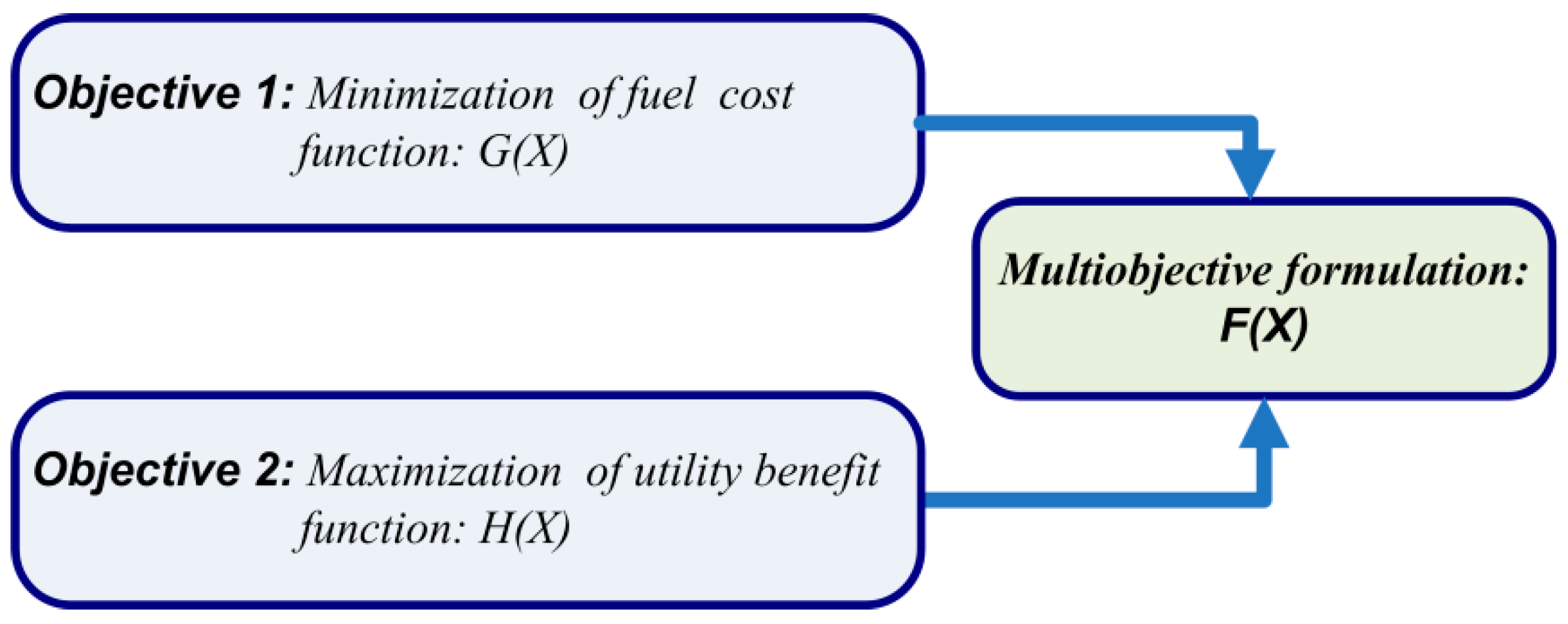
3.1. Objective1: Minimization of the Fuel Cost Function, G(X)

In this mode the reduction of the fuel cost of microgrid generators is the main objective. In this work, a power exchange scheme is assumed to exist between the main grid and microgrid. This scheme is needed to cater to the intermittent nature of renewables. When the microgrid system is not able to complete the load demand then power has to be taken from the main grid, and if the microgrid supply is a surplus with respect to its need then the excess power is given back to the main grid. Thus, this power exchange cost needs to be considered during modeling of the function to minimize the fuel cost of conventional generators of the microgrid. Equation (3) represent the required mathematical model of this cost function where $C_r\left(P{r}_t\right)$ is the cost of transferable power. $“{\gamma }_t”$, (dollars per kWh) is the rate of power exchange at a specific bus [12], whereas $(P_{rt})>0$ and $(P_{rt})<0$ reflect the power transfer between the microgrid and main grid, while the condition $(P_{rt})=0$ reflects there is no power exchange between the grid and microgrid. Positive and negative values reflect monetary gain and loss. The function related to minimization of fuel cost in this mode is as follows:

$$\min G\left(X\right)={\displaystyle \sum }_{t=1}^T\left(Cos{t}_t\right)=\min \left\{{\displaystyle \sum }_t^T{\displaystyle \sum }_l^L{C}_l\left(P_{l,t}\right)+{\displaystyle \sum }_1^T{C}_r\left(P{r}_t\right)\right\}$$

(2)

$$\mathrm{where}{C}_r\left(P{r}_t\right)=\{\begin{array}{c}(P_{rt})({\gamma }_t)if(P_{rt})>0\\ zeroif(P_{rt})=0\\ (P_{rt})(-{\gamma }_t)if(P_{rt})<0\end{array}$$

(3)

where $l,t,T,L$ hold integer values only:

• $l$: Variable to represent conventional generating units. Its value ranges from $1\le \mathrm{l}\le \mathrm{L}$;
• $t$: Dispatch interval, $1\le t\le T;$ in present work, is expanded over T = 24 time horizon.
• G(X): Operating cost function.
• $Cos{t}_t$: Total cost at time t to deliver power;
• $P_{l,t}$: Conventional generator, number of units;
• $C_l\left(P_{l,t}\right)$: Fuel cost function for conventional generators.
• $C_r\left(P{r}_t\right)$: Transferable power cost;
• $P_{rt}$: Transferable power;
• $\gamma$: Location marginal prices [33];
• $L$: Total number of the conventional generating unit.

Equation (2) subjected to following constraint:

$$\left\{{\displaystyle \sum }_{l=1}^L(P_{l,t})\right\}+\left\{P{s}_t+P{w}_t+P{r}_t\right\}+\left\{{\displaystyle \sum }_{i=1}^n(x_{j,t})\right\}-D_t=0$$

(4)

$$P_{l,\min }\le P_{l,t}\le P_{l,\max }$$

(5)

$$0\le P{s}_t\le S_t$$

(6)

$$0\le P{w}_t\le W_t$$

(7)

$$-P{r}_{\max }\le P{r}_t\le P{r}_{\max }$$

(8)

$$-D{R}_l\le P_{l,t+1}-P_{l,t}\le U{R}_l$$

(9)

where:

• i: Customer number;
• n: Total number of customers;
• $x_{i,t}$: Curtailed power by customer number i, at tth time interval
• $W_t$: Forecast maximum wind power obtainable by available solar energy generators;
• $S_t$: Forecast maximum solar power obtainable by available wind energy generators;
• $P_{wt}$: Wind generator power availability (during time t)
• $P_{St}$: Solar generator power availability (during time t)
• $D_t$: Load demand at time t;
• $P{r}_{max}$: Denotes maximum allowable exchange between grid and microgrid.

Equation (4) signifies the power balance. Collective generation of a conventional microgrid must fulfill all demand inside the microgrid. A small three-feeder radial low voltage scheme is taken in the present study. Losses for the model under consideration are assumed as having very low numeric value. The rest of the constraints are for power generation capacity of conventional and renewable power generators. The constraint, defined by Equation (5), is for generation limits of the conventional generators. This ensures that limits are not violated. Constraints defined using Equations (6) and (7) stand for renewable energy generators to ensure that the optimal values for renewable energy generators are within the forecast range. The fourth constraint, Equation (8), is to restrict the exchange of power. The sixth constraint, Equation (9), takes care of the maximum allowed ramp up and down rates.

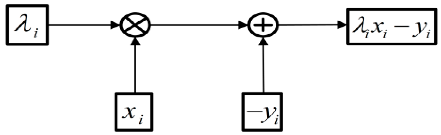
3.2. Objective2: Maximization of Utility Benefit Function, H(X), Using Demand Response

In general, demand response is viewed as the involvement of the end-user in the power system. This involvement is in the form of cost variation with time and obtained incentive. Demand response can be divided into two classes: the first one based on incentive, and the second based on a time-based rate program [34,35]. In this work we have adopted the first one.

The main interest of the utility is to maximize its benefit. The mathematical model of the function to represent this interest may be modeled as Equation (10). In the present work, we categorized electricity consumers in three different categories, and the following equations demonstrate the modeling for their behavior.

In this work, the quadratic outage cost function for more than one customer is used [36]. Equation (12) defines the customer cost function, where the “Z” term sorts users according to $\theta$, whereas $\theta$ is giving information about the user type and this information is used to categorize the customers [36,37,38,39]. Details of parameters related to the customer cost function are tabulated in Table 2. Customer benefit is defined as the difference between the incentive received by him and the cost incurred by him. Utility benefit can be stated as the difference between the cost of the load curtailed by user and the incentive obtained by the user. The mathematical model of the benefit function is as follows:

Benefit function of the utility:

$$V_2=\lambda x-y$$

(10)

Equation (10) denotes the benefit function of the utility where term “$\lambda x$” is the total hourly benefit to the utility when it does not deliver $“x”$ kW power to a specific customer at the rate of $“\lambda ”$ dollars per kWh [12]. The term y is compensation in terms of incentive which is paid to customer for reducing its load by $“x”$ kW.

Benefit function of the customer:

$$V_1=y-c$$

(11)

where:

• $V_1$: Customer benefit in $\$/\mathrm{kWh}$. It must be $V_1\ge$ 0 for user participation.
• $V_2$: Utility benefit in $\$/\mathrm{kWh}$.
• $x$: Curtailed power by customer in kW;
• y: Monetary compensation the customer receives in $/kWh;
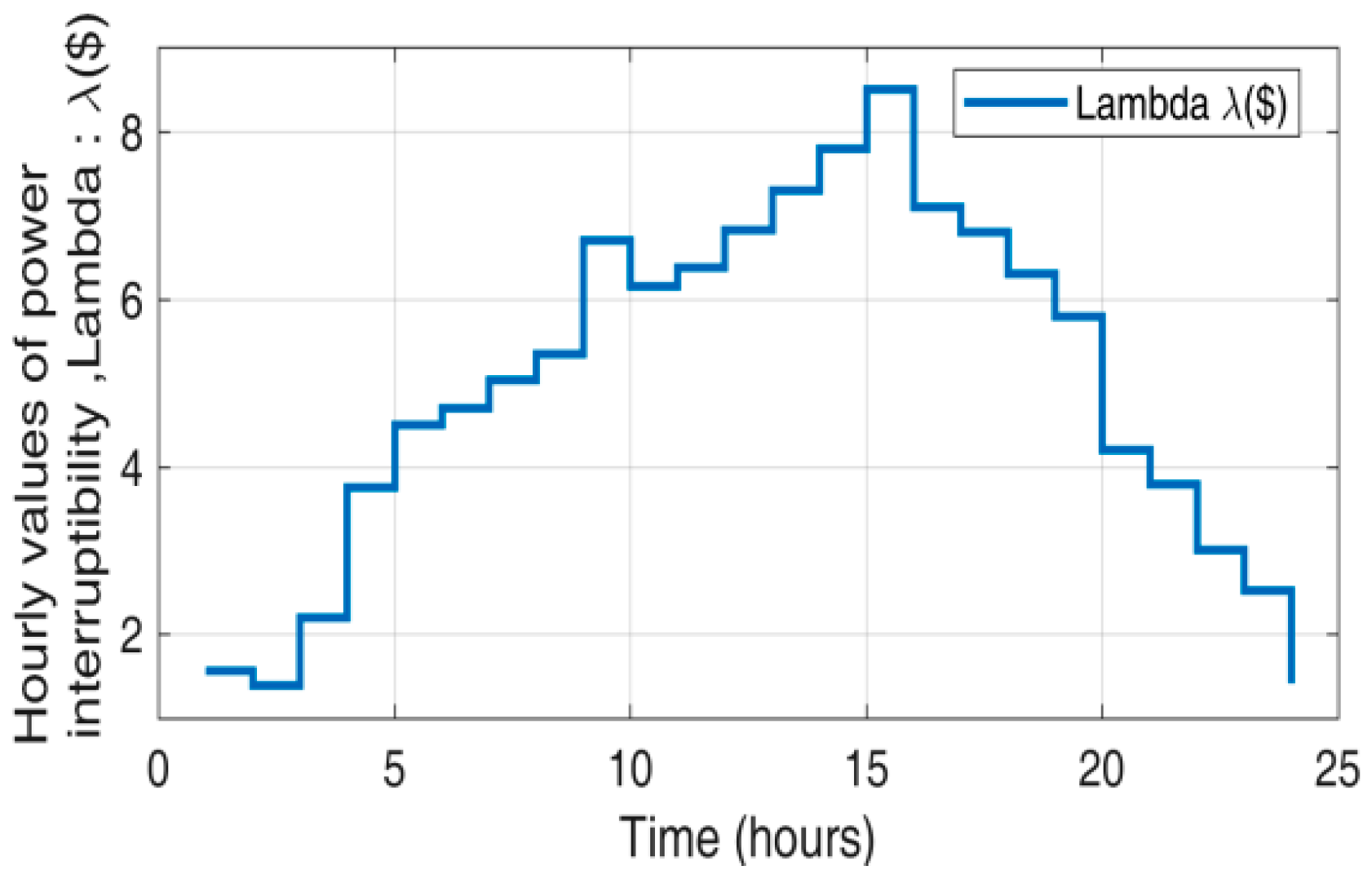
• λ: Cost of power.

Equation (11) denotes the benefit function ($V_1$) of the customer, where $c$ is the monetary loss to the user who reduces his power requirement by $“x”$ kW when DSM is applied and “y” is monetary incentive value that the customer receives. The customer would only participate if $V_1\ge 0$, meaning he gets some benefit.

The customer cost function for the ith customers can be modeled as:

$$c_i=A+B-Z$$

(12)

$$\begin{array}{l}A=K_{1,i}{x}_i^2,B=K_{2,i}{x}_i,Z=K_{2,i}{x}_i{\theta }_i\end{array}$$

(13)

and K_1,i, K_2,i are coefficients related to the costincurred by customer i.

The main interest of the utility is to maximize its benefit ($V_2$). If the number of users is “$i$” then it can be mathematically expressed as $\max \left({\lambda }_i{x}_i-y_i\right)$. A block diagram representation of this expression is shown by Figure 6.

The above demand response model maximizes the expected benefit for the utility when implemented over the total optimization period of twenty-four hours. With considering maximum powertarget and the total budget as practical constraintsit can be modeled as:

$$\max H\left(X\right)=\max {\displaystyle \sum }_{t=1}^{T=24}{\displaystyle \sum }_{i=1}^n[{\lambda }_{i,t}{x}_{i,t}-y_{i,t}]$$

(14)

subject to:

$${\displaystyle \sum }_{t=1}^T[y_{i,t}-\{(K_{1,i}{x}_{i,t}^2)+(K_{2,i}{x}_{i,t})-(K_{2,i}{x}_{i,t}{\theta }_i)\}]\ge 0$$

(15)

$$\begin{array}{c}{\displaystyle \sum }_{t=1}^T[y_{i,t}-\{(K_{1,i}{x}_{i,t}^2)+(K_{2,i}{x}_{i,t})-(K_{2,t}{x}_{i,t}{\theta }_i)\}]\\ \le {\displaystyle \sum }_{t=1}^T[y_{(i-1),t}-\{(K_{1,(i-1)}{x}_{i,t}^2)+(K_{2,(i-1)}{x}_{i,t})-(K_{2,(i-1)}{x}_{(i-1),t}{\theta }_{(i-1)})\}]\end{array}$$

(16)

$${\displaystyle \sum }_{t=1}^T{\displaystyle \sum }_{i=1}^n{y}_{i,t}\le TB$$

(17)

$${\displaystyle \sum }_{t=1}^{24}{x}_{i,t}\le C{P}_i$$

(18)

where $i,n,t,T$ hold integer values only, and i ranges between $1\le i\le n$, in Equation (15) and $2\le i\le n$, in Equation (16), and $“TB”$ denotesthe total budget of the utility. The daily limit of power interruptibility for customer $i$ is denoted by $C{P}_i$. Equation (15) denotes the constraint which restricts the incentive of an end-user on a daily basis. The constraint of Equation (16) is to restrict the customer benefit, which must be greater for greater curtailed customer power. The constraint denoted by Equation (17) limits the total utility payment to end-users as an incentive within its budget. The constraint represented by Equation (18) controls the individual curtailed customer power (on total time horizon).

3.3. Multi-Objective Formulation

The DSM problem in this paper involves two objectives, fuel cost minimization and utility benefit maximization. Putting Equations (2) and (14) together represents the DSM problem as a multi-objective optimization problem. However, the optimization tool adopted in this paper is TLBO, which is a single-objective optimization algorithm.

Thus, to implement TLBO both of the functions need to be converted into the same type. We converted the objective represented by Equation (14) from a maximization problem to a minimization problem by multiplying it with (−1). This transformation is represented in Equation (19).

The two objectives represented by Equations (2) and (19) are scalarized by pre-multiplying each of them with a weighing factor $“w”$ and $“\left(1-w\right)”$ such as the total weight: $w+\left(1-w\right)=$ The overall single-objective optimization problem is represented by Equation (20):

$$\min {\displaystyle \sum }_{t=1}^{T\left(=24\right)}{\displaystyle \sum }_{i=1}^n\left(y_{i,t}-{\lambda }_{i,t}{x}_{j,t}\right)$$

(19)

$$\min F\left(X\right)=\min [\left(w\right)\left\{{\displaystyle \sum }_{t=1}^T{\displaystyle \sum }_{i=1}^n{C}_l\left(P_{l,t}\right)+{\displaystyle \sum }_1^T{C}_r\left(P{r}_t\right)\right\}+\left(1-w\right)\left\{{\displaystyle \sum }_{t=1}^{T\left(=24\right)}{\displaystyle \sum }_{j=1}^n\left(y_{i,t}-{\lambda }_{i,t}{x}_{i,t}\right)\right\}]$$

(20)

where $x_{i,t}$, $y_{\mathrm{i},t}$, $P_{w,t},P_{s,t}$, $P_{r,t}$, $P_{l,t}$ are decision variables.

In this work we transformed the constrained objective function into the unconstrained objective by adding penalty terms for each constraint violation (Equations (4)–(9) and (15)–(18)). In the present work we a have given equal weighting to both objectives.

There are many methods to handle the constraint of an objective function in an optimization problem. In the present work, we designed the constraints of our objective function using an exterior penalty approach in which infeasible design variables are penalized, but feasible design variables are not penalized [40].

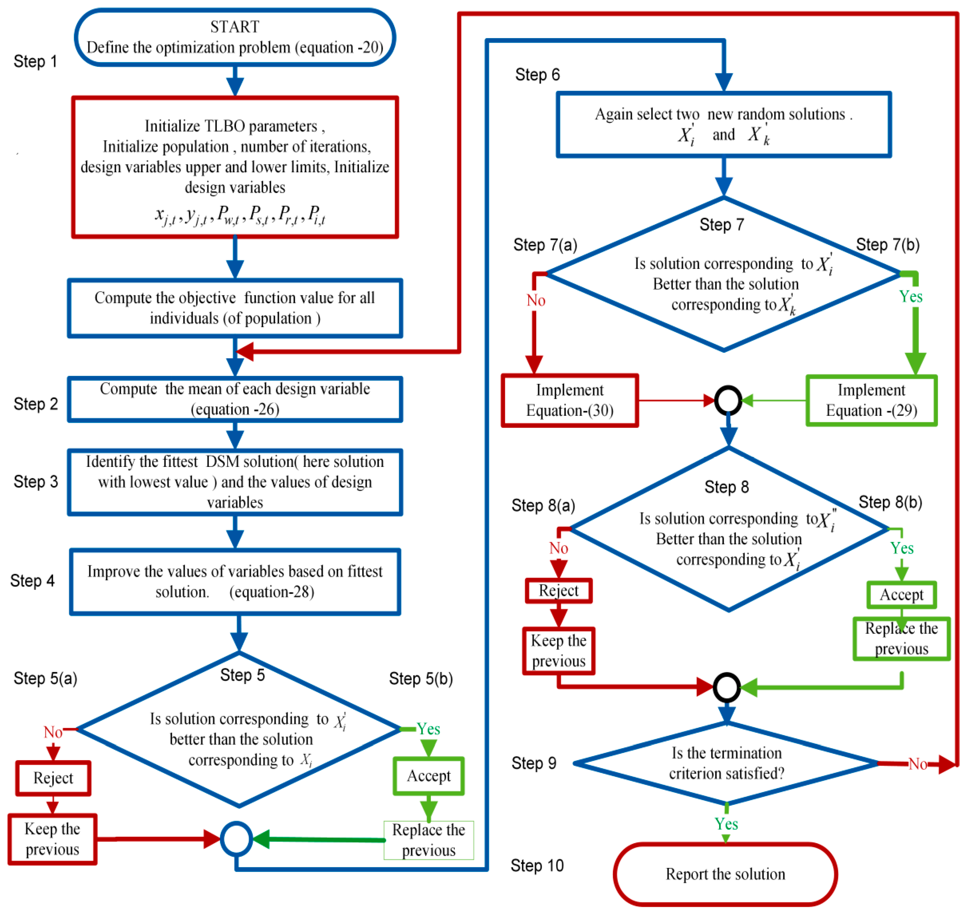
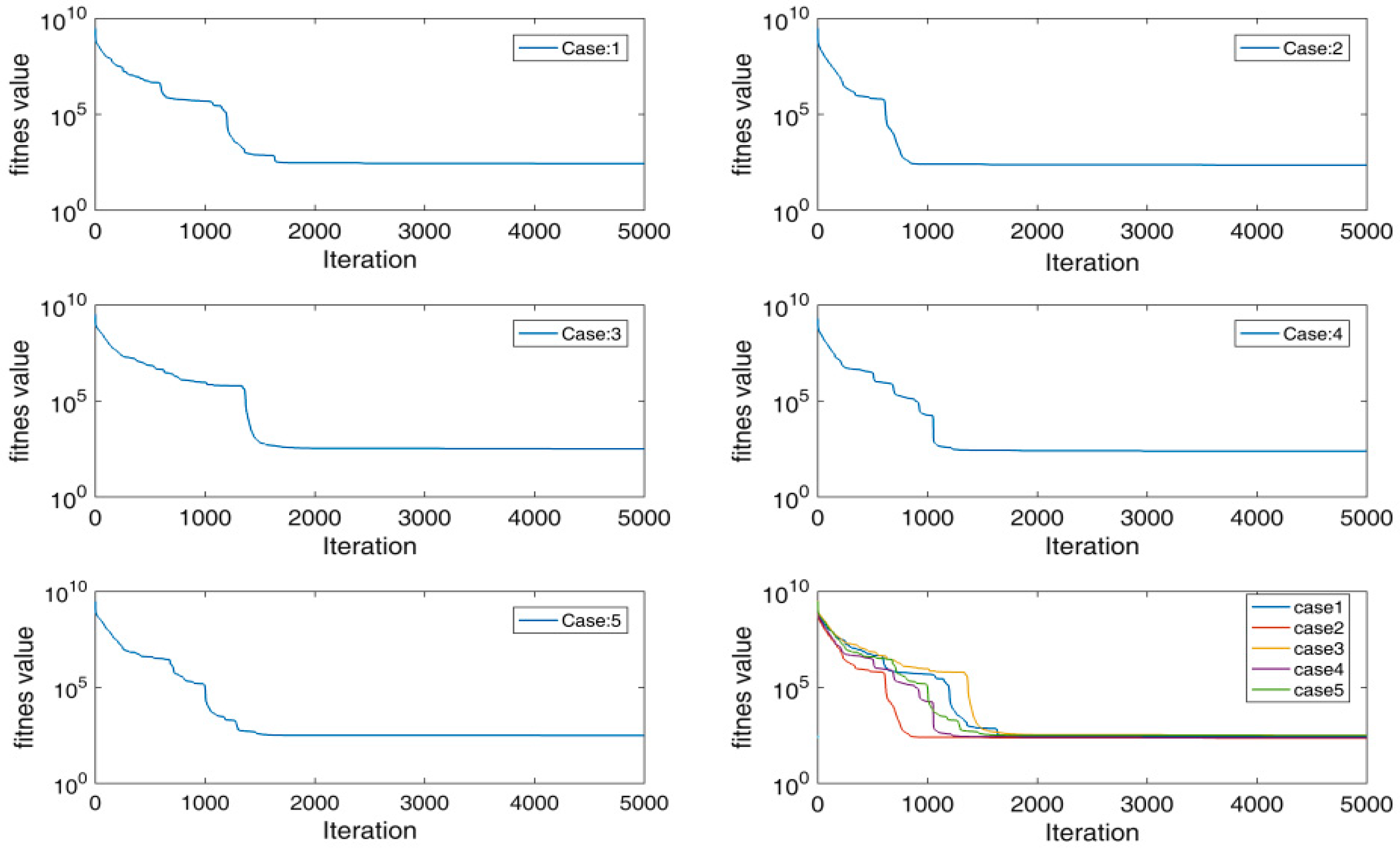
4. Teaching-Learing-Based Optimization (TLBO) Algorithm

Under this section TLBO is first introduced, and then its adaptation for multi-objective formulation has been presented.

In [29] six different meta-heuristic algorithms including TLBO are compared. These algorithms are, namely, Whale Optimization, Fire Fly, PSO, Differential Evaluation, and GA. This compression is done mainly in terms of selecting the best suitable optimization method for cost minimization of the micro-grid. In terms of convergence characteristics analysis among these methods TLBO reported the fastest convergence. Search agents of TLBO are found more effective to explore the feasible search space. It is reported in the [29] that TLBO search agents require the least effort. Among the above-mentioned six meta-heuristic techniques TLBO is reported as the best in most of the conditions.

The microgrid DSM is a multi-objective problem, and TLBO is a promising method for optimization. TLBO is proposed by [27,28]. The algorithm is divided in two phases, namely, teacher and learner. This phase of TLBO is explained below.

A. Teacher Phase:

In this phase a teacher tries to improve the average result of the class in his subject. In this identification of the best solution from the population is done on the based on the objective function value.

If $X_{k,i}$ is the fittest solution at any iteration $i$ then it can be represented as $X_{j,kbest,i}$. Calculation of the mean result of the learner, in a subject j will be done in the next step. The effort of the teacher to improve the mean result of the class in his subject depends on the capability of the teacher. This improvement in the existing mean result is modeled as:

$$Difference\_Mea{n}_{j,k,i}=r_{j,i}(X_{j,kbest,i}-T_f{M}_{j,i})$$

(21)

where:

• $X_{j,kbest,i}$: Result of the best learner in subject j;
• $r_{j,i}$: Random number in the range [0, 1]; and
• $T_f$: Teaching factor. It decides the value of mean to be changed the value of $T_f$ is selected in random way with equal probability as:

$$T_f=round\left[1+rand\left(0,1\right)\left\{2-1\right\}\right]$$

(22)

updated solution in the teacher phase:

$$X{\prime }_{j,k,i}=X_{j,k,i}+Difference\_Mea{n}_{j,k,i}$$

(23)

where:

• $X_{j,k,i}$: A value in the solution,
• $X{\prime }_{j,k,i}$: Updated value of $X_{j,k,i}$. Accept $X{\prime }_{j,k,i}$ if it gives better value of the function
• $j$: jth design variable. Denotes subject chosen by the learners. $j=1,2,\dots ,m$;
• k: kth member of population. Denotes learner. $k=1,2,\dots ,n$;
• i: ith iteration, $i=1,2,\dots ,G_{\max }$,
• $G_{\max }$: Denotes maximum iterations.

All the values of the function accepted in this phase are reserved and treated as the learner phase input.

B. Learner phase:

In this phase learners improve their knowledge by interaction. A population size of $\mathrm{n}$ is considered. At any iteration, random compression between learners is done. Random selection of two learners is conducted, namely, P and Q. For these two randomly-selected learners ${X^{\prime }}_{P,i}\ne {X^{\prime }}_{Q,i}$. Updated values of the first phase:

$${X^{″}}_{j,P,i}=\{\begin{array}{c}{X^{\prime }}_{j,P,i}+r_{j,i}\left({X^{\prime }}_{j,P,i}-{X^{\prime }}_{j,Q,i}\right),f\left({X^{\prime }}_{P,i}\right)<f\left({X^{\prime }}_{Q,i}\right)\\ {X^{\prime }}_{j,P,i}+r_{j,i}\left({X^{\prime }}_{j,Q,i}-{X^{\prime }}_{j,P,i}\right),f\left({X^{\prime }}_{P,i}\right)>f\left({X^{\prime }}_{Q,i}\right)\end{array}$$

(24)

${X^{″}}_{j,P,i}$ is accepted if it provides a better function value. Accepted function values at the end of the learner phase are reserved and treated as the input of the next iteration.

The steps involved in programming for TLBO implementation in presented paper and its flow chart are given in below section.

TLBO Steps Adopted to Optimize Multi-Objective DSM Function F(X)

In this section step needed to adopt TLBO to optimize F(X) is presented first and followed by its flow chart illustration as given in Figure 7.

Step1: Initialize population, design variables (X) of DSM program, and termination criterion:

$$X=\left[P_{l,t}{P}_{r,t}{P}_{w,t}{P}_{s,t}{x}_{i,t}{y}_{i,t}\right]$$

(25)

Step2: Calculate the mean of each design variable:

$$DiffrenceMean=r\left(X_i\left(s\right)-T_f\overline{X}\left(s\right)\right)$$

(26)

In the above equation $\overline{X}\left(s\right)$ mean the result while $“r”$: random number, $\in$ [0, 1]. The value of $T_f$ determined randomly as:

$$T_f=round\left[1+rand\left(0,1\right)\left\{2-1\right\}\right]$$

(27)

Step3: Determine the fittest solution.

Step4: Improve the solution according to the fittest solution:

$${X^{\prime }}_i\left(s\right)\leftarrow X_i\left(s\right)+r\left(X_i\left(s\right)-T_f\overline{X}\left(s\right)\right)$$

(28)

Step5: Determine the better solution between ${X^{\prime }}_i$ and $X_i$.

Step5(a): If the above condition is not satisfied then reject the new result and keep the previous one and go to the next step.

Step5(b): If the condition is satisfied then accept the new one by replacing the old and go to step6.

Step6: Choose two random solution ${X^{\prime }}_i\mathrm{and}{X^{\prime }}_k$.

Step7: Determine fittest solution between ${X^{\prime }}_i\mathrm{and}{X^{\prime }}_k$.

Step7(a): If ${X^{\prime }}_i\mathrm{is}\mathrm{better}\mathrm{than}{X^{\prime }}_k$ then perform the update below and go to Step8:

$${X^{\prime }}_i\left(s\right)+r\left({X^{\prime }}_i\left(s\right)-{X^{\prime }}_k\left(s\right)\right)\to {X^{″}}_i\left(s\right)$$

(29)

Step7(b): If ${X^{\prime }}_i\mathrm{not}\mathrm{better}\mathrm{than}{X^{\prime }}_k$ than perform the below update and go to the next step.

$${X^{\prime }}_i\left(s\right)+r\left({X^{\prime }}_k\left(s\right)-{X^{\prime }}_i\left(s\right)\right)\to {X^{″}}_i\left(s\right)$$

(30)

Step8: Is solution ${X^{″}}_i\mathrm{better}\mathrm{than}{X^{\prime }}_i$?

Step8(a): If the condition is not satisfied then reject ${X^{″}}_i$, keep ${X^{\prime }}_i$ and go to step9.

Step8(b): If the condition is satisfied then accept ${X^{″}}_i$, replace ${X^{\prime }}_i$ and go to the next step.

Step9: Is the termination criteria satisfied? If the answer is yes then go to the next step; otherwise start the whole process again from step2.

Step10: Report the optimum solution.

5. Object-Oriented Usability Indices (OOUI)

Under this section the proposed indices are defined and discussed.

Peak load shaving and increased integration of renewable sources were identified as the main objectives of a demand-side management program. A usability index is expected to present the fulfillment of these two objectives in any specific case study via quantified numerical factors. The outcome of any demand response program does not contain any such indices directly based on which the relative fulfillment of these objectives could be identified. In the absence of such indices, the policy decision of going with demand-side management may not produce the optimized result all the time. Therefore, OOUI are proposed in this section to indicate the relative fulfillment of the two main objectives.

In a power network, the electricity demand varies with time which is presented through the load profile. The power operator faces a challenge of balancing load and generation when peak load conditions appear. Demand-side management, when appropriately performed, reduces some load in peak hours and relieves the operator’s stress. Load factor, which is the ratio of the average load on the generator over a period of time to the peak load in the same time interval, indicates the variability of the load. A low load factor indicates that the load is highly variable. A high load factor is desirable for the economic feasibility of plant.

If a demand response program performs as per the requirements, it should reduce the load in peak hours and, therefore, the load factor should improve after allying DSM. A peak power shaving factor is defined as:

$$m_{pps}=\frac{L{F}_{\mathrm{DSM}}}{L{F}_{\mathrm{WDSM}}}$$

(31)

where $L{F}_{\mathrm{DSM}}$ is the load factor of the power network when DSM is applied and $L{F}_{\mathrm{WDSM}}$ is the load factor of the power network when it operates without demand response. If DSM successfully shaves the load in peak hours, then the load factor will improve and the peak power shaving index will be greater. For better peak power shaving operation, $m_{pps}$ should be as high as possible.

Renewable energy generators are often small in size and unpredictable in terms of availability. Therefore, the generation support from these sources may or may not always be helpful for the power operator. A good demand response program, in terms of renewable energy integration, is one which ensures a good amount of load satisfied with renewable energy sources. A renewable energy integration index indicates the percentage utilization of electrical energy from renewable-based sources. This index is given as:

$$m_{rei}=\frac{P_{gr}}{P_{gt}}$$

(32)

where $P_{gr}$ active power is supplied by renewable energy sources and $P_{gt}$ is the total active power supplied.

An overall usability index which indicates the fulfillment of both the objectives of DSM presented by OOUI. Depending upon the specific system architecture and policy-related decisions, the relative weighting of these two indices may vary. Therefore, the overall usability index also includes the individual weighting and is defined as:

$$m_{dsmuf}=w_{pps}{m}_{pps}+w_{rei}{m}_{rei};\mathrm{where}{w}_{pps}+w_{rei}=1;$$

(33)

Above, $w_{pps}$ and $w_{rei}$ are the relative weighting of the peak power shaving index and renewable energy integration index, respectively.

Theoretical Analysis of the Proposed Indices

This section presents the theoretical analysis of proposed indices. First of all, the analysis of the peak power shaving index is presented, and then the renewable energy integration index is analyzed. Finally, the overall usability index is analyzed.

Let load demand to utility over a time interval T is given as:

$$d_t=\left[d_1,d_2,d_3,\dots \dots ,d_T\right],tЄT$$

(34)

where $d_1,d_2,d_3,\dots \dots ,d_T$, are loads during 1st, 2nd, 3rd… and Tth, dispatch intervals (in the presented work hourly load variation with dispatch intervals of one hour are considered (Figure 3a). Average load demand to utility over time period T is calculated using the expression:

$$\frac{1}{T}{\displaystyle \sum }_{t=1}^{T=24}{d}_t$$

(34a)

Now the load factor with DSM ($L{F}_{\mathrm{DSM}}$) and without DSM ($L{F}_{\mathrm{WDSM}})$ is calculated using the following expression:

$$L{F}_{\mathrm{WDSM}}=\left(\frac{1}{T}{\displaystyle \sum }_{t=1}^T{d}_t/d_{\max }\right)\mathrm{and}L{F}_{\mathrm{DSM}}=\left(\frac{1}{T}{\displaystyle \sum }_{t=1}^T{d}_t^{\prime }/d_{\max }^{\prime }\right)$$

(35)

where:

• t: dispatch interval.
• $d_t$: load demand to utility when no DSM is applied.
• $d_{max}$: maximum load over the time period T when no DSM is applied
• $d_t^{\prime }$: load demand to utility when DSM is applied.
• $d_{max}^{\prime }$: maximum load over the time period T when DSM is applied

$m_{pps}$ is defined as the ratio of $L{F}_{\mathrm{DSM}}/L{F}_{\mathrm{WDSM}}$. This can be represented as:

$$m_{pps}=\left(\frac{1}{T}{\displaystyle \sum }_{t=1}^T{d}_t^{\prime }/d_{\max }^{\prime }\right)/\left(\frac{1}{T}{\displaystyle \sum }_{t=1}^T{d}_t/d_{\max }\right)$$

(36)

Any index proposed as an indicator of DSM usability should quantify the obtained benefit. One of the main purposes of DSM is to reduce the stress on the operator. The sudden high demand from the load in some hours of operation puts stress over the system. Therefore, the index which shows the benefit in terms of reduction of load should be an indicator.

Peak power index analysis can be done under the following points:

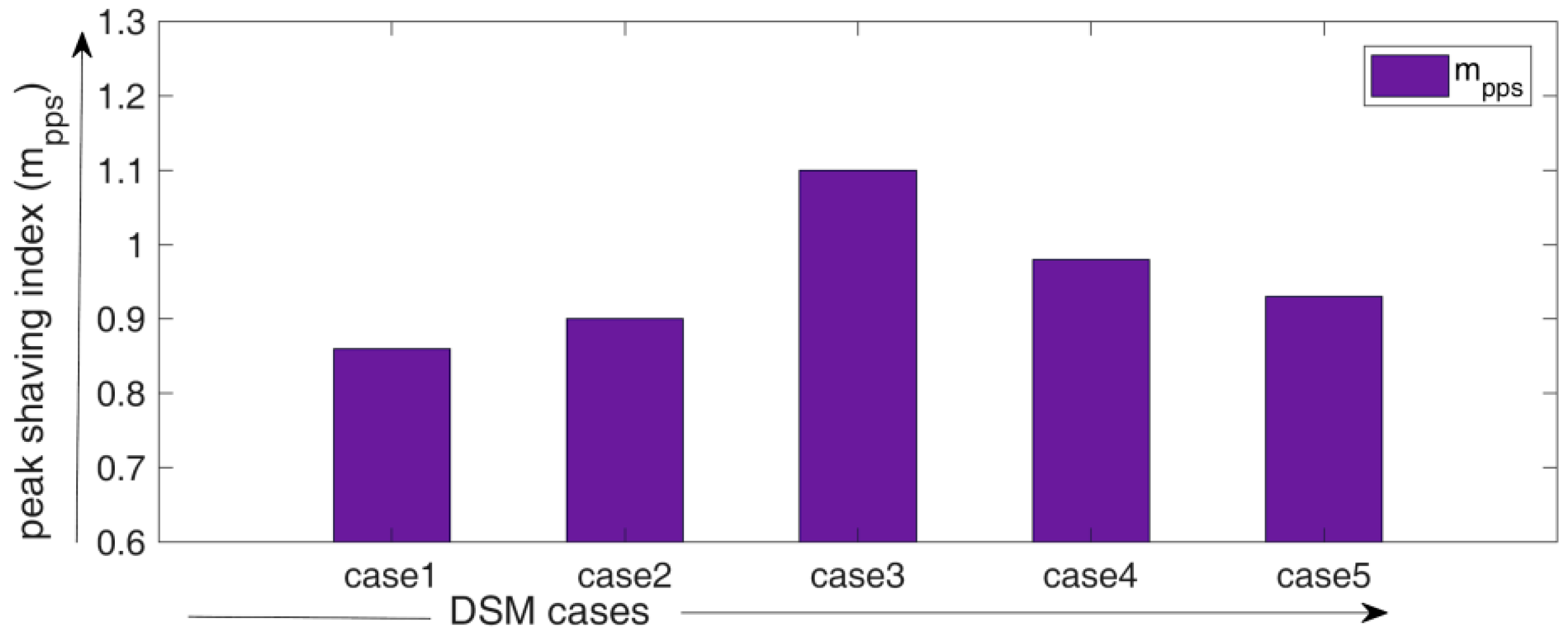
• Peak power shaving index greater than one that is $m_{pps}>1$.
• Peak power shaving index less than one that is $m_{pps}<1$.
• Peak power shaving index equal one that is $m_{pps}=1$.
• Comparative result of peak power shaving index obtained for DSM solutions.

The first condition, $m_{pps}>1$, will arise if the load factor with DSM ($L{F}_{\mathrm{DSM}}$) is higher than the load factor without DSM ($L{F}_{\mathrm{WDSM}}$). In this condition the value of the peak power shaving index will be higher. Here, the value of $m_{pps}$ indicates how much improvement is achieved in terms of load factor after implementing DSM.

The second condition, $m_{pps}<1,$ will arise if the load factor with DSM ($L{F}_{\mathrm{DSM}}$) is lower than the load factor without DSM ($L{F}_{\mathrm{WDSM}}$). In this condition the value of the peak power shaving index will be lower than 1. The value of $m_{pps}$ in this condition indicates a decrease in the load factor value with respect to the without-DSM case.

The third condition, $m_{pps}=1,$ will arise if the load factor with DSM ($L{F}_{\mathrm{DSM}}$) is equal to the load factor without DSM ($L{F}_{\mathrm{WDSM}}$). This also indicates that the load factor without DSM is equal.

If the peak power shaving index is calculated and presented for different solutions of DSM, then its relative higher value indicates a better load factor compared to the DSM outcome in other cases. Coincidently, if all DSM solutions are equally good considering load reduction, then the higher value of the peak power shaving index in a specific DSM program can give a ranking of achieved relative peak shaving.

The following example gives an illustrative view about the application of the peak power shaving index. Let us assume that there is a DSM scheme, F(X), for a grid-tied microgrid. This DSM is adopted for five different availability conditions of renewable energy. These conditions are named as case 1, case 2, case 3, case 4, and case 5. The proposed peak power shaving index is calculated for each case and their values are presented as ‘$m_{pps}$’.

If the operator wants to know that, among all five cases, in which case maximum peak shaving has been achieved, the answer can be provided by the values of $m_{pps}$. To demonstrate the working of $m_{pps}$, a bar chart is plotted. Indicator values as given in Figure 8 represent that in case 3 the peak power shaving index hold maximum value which indicate that the percentage contribution of peak power shaving is the maximum in case 3 relative to other DSM cases. Additionally, the higher value of case 3 indicates that the load factor in this case with respect to other cases is much better.

The ratio of active power from renewables ($P_{gr}$) to total active power $\left(P_{gt}\right)$ quantifies the involvement of renewable energy. Suppose if the value of this index is 0.26, then it means renewable energy contribution in this case to fulfill total demand is 26%. The lowest possible value for this index can be zero, which will indicate the condition of no-contribution of renewable energy in fulfilling the demand. If the value of $m_{rei}$ is equal to one than it mean 100% renewable energy is used to fulfill all the demand.

If the operator wants to know that, among all cases, which one achieves relatively major integration of renewable energy sources while implementing DSM, $m_{rei}$ can help here by providing a numerical value in the form of an index. The DSM case with a higher value of $m_{rei}$ involves a greater renewable energy percentage to fulfill load demand.

An overall usability index indicates DSM usability combined with peak load shaving and renewable energy integration. Depending upon the specific system architecture and policy-related decisions, the individual weighting of $m_{pps}$ and $m_{rei}$ may vary.

In extreme cases, if the weight associated with $m_{rei}$ is set at 0 and the weight associated $m_{pps}$ is set at 1, then the overall usability index (represented by $m_{dsmuf}$) becomes equal to the peak power shaving index. Thus, it indicates that the desired aim of DSM is only to take care of peak power shaving. Similarly, if this extreme setting is interchanged for DSM, it can be concluded that the DSM scheme is only focusing on renewable energy integration and has zero interest in achieving load factor improvement or peak power shaving.

6. Case Studies, Simulation Results, and Discussion

Under this section we first present the different renewable energy availability cases. Simulation results of the multi-objective formulation of the DSM using the TLBO method in the MATLAB environment is presented next. Finally, determination of OOUI, followed by a discussion, is conducted.

Figure 9 represents the approach adopted in the presented work with respect to the application and usability of the proposed indices. First of all, a microgrid multi-objective DSM formulation ($F\left(X\right)$) is conducted. In the next step the TLBO algorithm is adopted to solve $F\left(X\right)$, and the optimized results are obtained. From these solutions the proposed OOUI are calculated and made available to the operator. A MATLAB-based simulation has been performed to obtain all of the simulation results.

It is considered that the participation of all loads is equally shared, and each type of load has equal right to make a decision to get involved in the demand response program. The microgrid operator has the information about the interruptible energy limit of the user on per day bases and this information is used to index the end users in order of increasing interest to diminish their energy need. Additionally, the outage cost function coefficients $\left(K_{1,i}\mathrm{and}{K}_{2,i}\right)$ of involved users are considered to be known to the operator. The daily utility budget is $500.

6.1. Case Studies, Simulation Results

Solution of the multi-objective formulation of DSM is obtained using TLBO for five different scenarios of renewable energy availability in the microgrid. These scenarios are presented as cases 1–5. Case 1 deals with the condition of average wind and average solar availability; in this case total availability of renewable power is 346.24 kW. Case 2 considers the maximum wind and average solar availability and total renewable power availability in this case is 400.5 kW. Case 3 is when wind availability is at a minimum, and solar availability is average and overall availability of renewable sources is 275.03 kW. Average wind and maximum solar availability are termed as case 4; in this case renewable energy availability is 362.76 kW. Finally, case 5 deals with the generation scenario when the wind is average and solar has minimum availability, and the total availability of renewable energy is 296.01 kW. The solar power availability and wind power availability under different cases are represented in Figure 10 and Figure 11; these figures present the hourly variation of solar and wind energy availability in different cases.

Under all of these conditions the DSM program is run, and the iteration vs. fitness value plots are given in Figure 12. The results indicate that the optimization target is achieved around 2000 iterations in all cases. As a result of the optimization new load profiles are obtained for each case. These new load profiles are in accordance with the two objectives of F(X). These load curves for different cases are plotted and presented in Figure 13, with and without the DSM load curve. Values of parameters obtained from these load curves are listed in

Table 3. Load curve data for DSM cases 1–5.

Cases	Total Demand (kW)	Avg. Demand (kW)	Peak (kW)	Load Factor	Renewable Energy Availability
					(kW)	(%)
case 1	780.236	32.50983	39.25754	0.828117	346.24	34.62
case 2	793.9236	33.08015	41.66873	0.793884	400.45	40.04
case 3	767.8551	31.99396	39.95539	0.800742	275.03	27.50
case 4	771.3937	32.1414	40.25102	0.798524	362.76	36.27
case 5	775.5615	32.31506	39.35548	0.821107	296.01	29.60

. Total, average, and peak demand when DSM is not implemented is 864.9 kW, 36.0375 kW, and 42.09 kW, and the load factor is 0.84. These parameters are needed to calculate OOUI values.

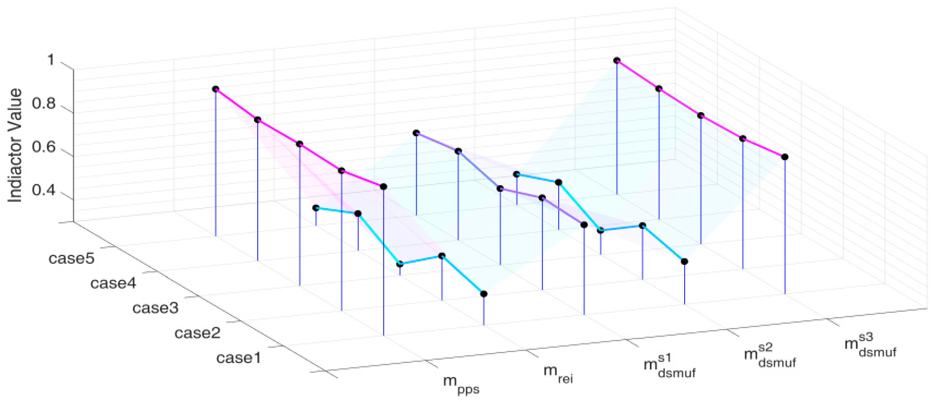
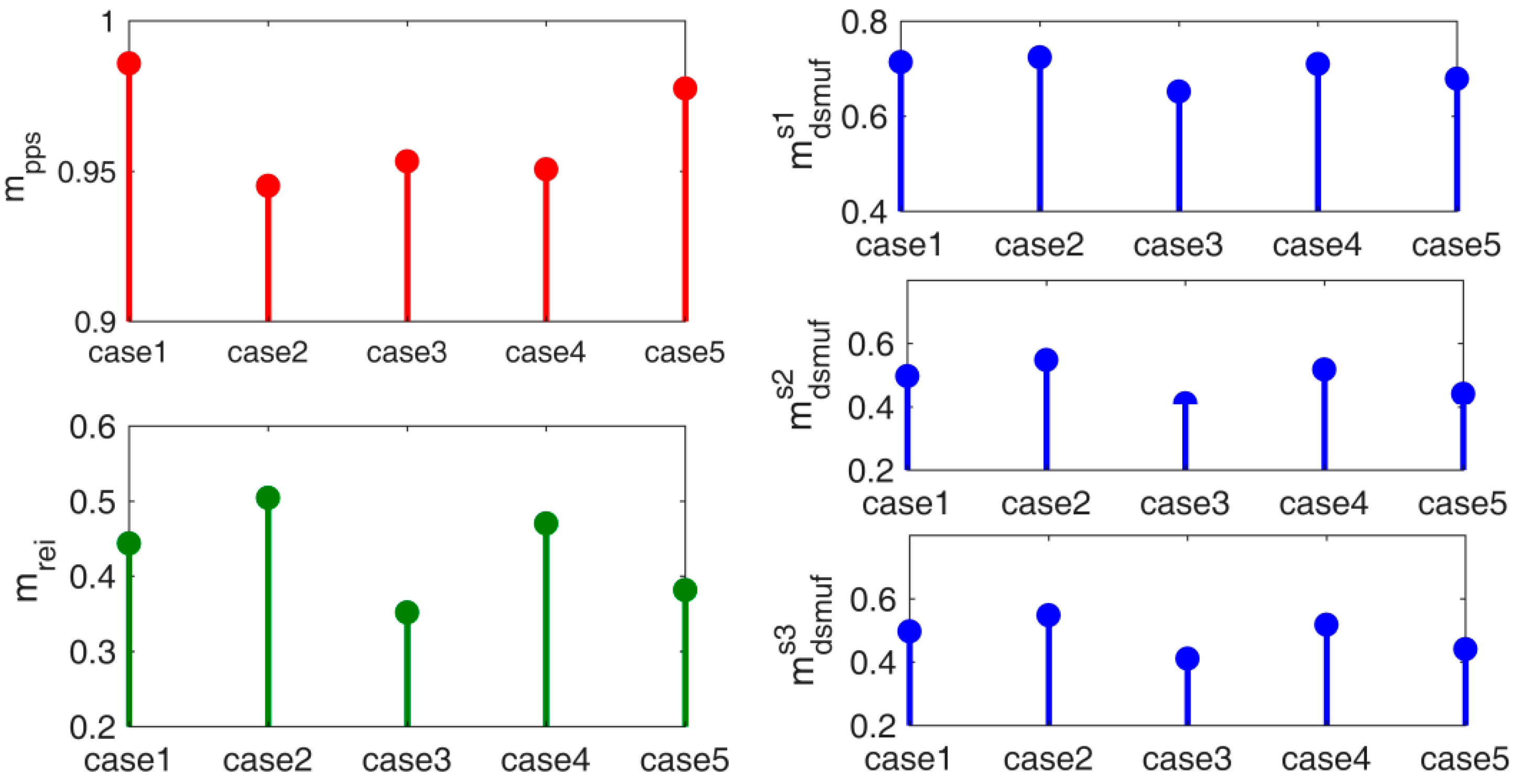
6.2. Calaulation of Proposed Indices

The calculations of the proposed indices are based on the mathematical relation as given in Section 5.

Table 4. OOUI for DSM.

Cases	$\mathbf{W}\left(\mathbf{k}\mathbf{W}\right)$	$\mathbf{S}\left(\mathbf{k}\mathbf{W}\right)$	${\mathit{m}}_{\mathit{p}\mathit{p}\mathit{s}}$	${\mathit{m}}_{\mathit{r}\mathit{e}\mathit{i}}$	${\mathit{m}}_{\mathit{d}\mathit{s}\mathit{m}\mathit{u}\mathit{f}}^{\mathit{s}1}$	${\mathit{m}}_{\mathit{d}\mathit{s}\mathit{m}\mathit{u}\mathit{f}}^{\mathit{s}2}$	${\mathit{m}}_{\mathit{d}\mathit{s}\mathit{m}\mathit{u}\mathit{f}}^{\mathit{s}3}$
					$({\mathit{w}}_{\mathit{p}\mathit{p}\mathit{s}}$$=0.5,{\mathit{w}}_{\mathit{r}\mathit{e}\mathit{i}}=0.5)$	$({\mathit{w}}_{\mathit{p}\mathit{p}\mathit{s}}$$=0.1,{\mathit{w}}_{\mathit{r}\mathit{e}\mathit{i}}=0.9)$	$({\mathit{w}}_{\mathit{p}\mathit{p}\mathit{s}}$$=0.9,{\mathit{w}}_{\mathit{r}\mathit{e}\mathit{i}}=0.1)$
Case 1	Average	Average	0.986	0.444	0.715	0.498	0.932
Case 2	Maximum	Average	0.945	0.504	0.725	0.548	0.901
Case 3	Minimum	Average	0.953	0.358	0.655	0.418	0.894
Case 4	Average	Maximum	0.951	0.470	0.711	0.518	0.903
Case 5	Average	Minimum	0.978	0.382	0.680	0.441	0.918

$W\mathrm{and}S$: Wind power availability forecast, while $\mathrm{S}$ denote Solar power availability forecast. $m_{rei}$: Renewable energy integration index; $m_{pps}$: Peak power shaving index. $w_{pps}$: Weighting of $m_{pps}$: and ${\mathrm{w}}_{\mathrm{rei}}$ for $m_{rei}$. $m_{dsmuf}$: Overall usability index. $m_{dsmuf}^{s1}$: It is $\mathrm{for}$ scenario 1. In this scenario weighting of two factors are $w_{pps}$ = 0.5 and $w_{rei}=0.5$. $m_{dsmuf}^{s2}$: It is $\mathrm{for}$ scenario 2. In this scenario weighting of two factors are $w_{pps}$ = 0.1 and $w_{rei}=0.9$. $m_{dsmuf}^{s3}$: It is $\mathrm{for}$ scenario 3. In this scenario weighting of two factors are $w_{pps}$ = 0.9 and $w_{rei}=0.1$.

presents the calculated values of these indices under all five cases studied.

The renewable energy integration index presents how much the participation of renewable sources has been achieved. The peak power shaving index indicates how much peak load shaving has been achieved. The overall usability index is calculated with the help of the weighted sum of these two indices.

This work considers three different weighting scenarios named as scenario 1, scenario 2, and scenario 3. In scenario 1, equal weighting $\left(w_{pps}=w_{rei}=0.5\right)$ is given to both objectives. In the second scenario, the renewable energy integration has been given higher weighting ($w_{rei}$ = 0.9). In the third scenario, the peak power shaving remains the preferred objective and has higher weighting ($w_{pps}$ = 0.9). Table 4 presents the calculated indices and overall index under all five cases of energy availability and weighting scenarios. The peak power shaving targets are achieved with the maximum amount in case 1 when wind and solar energy availabilities are average.

The next best case is case 4 when wind availability is average and solar energy is at maximum availability. This indicates that a significant amount of peak power shaving can be achieved when at least an average solar availability is ensured. The reason can be attributed to the solar availability in peak load duration. With average or maximum availability, solar provides additional support to conventional generators and the grid in easing the peak load conditions. Renewable energy utilization is another objective of DSM. The renewable energy integration index indicates the fractional quantity of renewable generation concerning a conventional generator. The calculated values indicate that maximum integration of renewable energy is achieved with DSM in case number 4, where wind availability is average and solar availability is the maximum. In general, the condition where both have maximum availability should be the best scenario for renewable energy utilization.

For such condition to occur, a combination of suitable weather conditions is required. Therefore, the next best situation is when one source generates the maximum and the other generates average energy. These two conditions occur in case 2 and case 4. However, as the values of the renewable energy integration index indicate, solar energy has more impact on fulfilling this target. When both the indices are combined to obtain a final index, which presents the object-oriented DSM usability, the condition for the maximum benefit of DSM is obtained. As can be seen from Table 3, the overall maximum benefit from DSM can be achieved in case 3, when wind provides minimum energy and solar provides average energy. This conclusion remains valid for any weighting given to either objective of DSM. Whether either objectives have equal weighting, or one of them has higher weighting, the best result can be obtained only in case number 3. This conclusion can help in policy-making while deciding to adopt the DSM for any specific system. Figure 14 and Figure 15 present the different indices in plots where the conclusion can be easily identified and established.

6.3. Discussion of the Results with Comparative Analysis

This section is divided into the following two parts: (A) The findings of the present work are discussed keeping the focus on the obtained values of the proposed indices for DSM; and (B) comparative discussion with similar studies published by other authors to show the uniqueness of the present work.

(A) Observation of Table 3 and Table 4, focusing on the numeric values of peak power shaving index, reveals two things: (1) regarding peak shaving and (2) the load factor. A close look of Table 3 and Table 4 shows that the peak shaving actor holds adirect relation with the load factor and a reciprocal relation with peak shaving. Observation of

Table 5. OOUI ranks of DSM.

Rank	Criteria for Ranking DSM
	${\mathit{m}}_{\mathit{p}\mathit{p}\mathit{s}}$	${\mathit{m}}_{\mathit{r}\mathit{e}\mathit{i}}$	${\mathit{m}}_{\mathit{d}\mathit{s}\mathit{m}\mathit{u}\mathit{f}}^{\mathit{s}1}$	${\mathit{m}}_{\mathit{d}\mathit{s}\mathit{m}\mathit{u}\mathit{f}}^{\mathit{s}2}$	${\mathit{m}}_{\mathit{d}\mathit{s}\mathit{m}\mathit{u}\mathit{f}}^{\mathit{s}3}$
1	Case 1	Case 2	Case 2	Case 2	Case 1
2	Case 5	Case 4	Case 1	Case 4	Case 5
3	Case 3	Case 1	Case 4	Case 1	Case 4
4	Case 4	Case 5	Case 5	Case 5	Case 2
5	Case 2	Case 3	Case 3	Case 3	Case 3

reveals that case 1 holds rank 1 when ranking is done on the basis of the peak power shaving index. This indicates that when DSM is applied to case 1 then it achieves maximum peak shaving in obtaining its objectives. Case 2 is ranked 5th on the basis of the peak shaving index value, which means that peak reduction is the minimum in this case. In case 2 the maximum peaks are 41.67 kW (Table 3) which is very close to without DSM load curve peak (42.09 kW). Figure 13 (case 2) shows that in this case DSM also reduces the overall demand and achieves its objectives, but is poor in terms of peak shaving. In terms of higher peak reduction, cases 1–5 can be arranged as follows: case 1 > case 5 > case 3 > case 4 > case 2.

Observation of Table 3 and Table 4, while focusing on the numeric values of renewable energy index, reveals that its value is the maximum in case 2 and the minimum in case 3. This indicates that the percentage contribution of renewable energy in fulfilling the total load demand is the maximum with respect to other cases.

In case 2 total power requirements for the users is 793.92 kW and the renewable energy integration index value is 0.504, which indicates that the contribution of renewable energy in the total requirement is 50.4%. Cases 1–5 can be arranged according to renewable energy contribution in their total demand as follows: case 2 > case 4 > case 1 > case 5 > case 3.

Observation of Table 4, while focusing on the numeric values obtained for the overall usability index, giving equal weighting (0.5) to peak power shaving and the renewable energy integration index shows that it holds a maximum value for case 2 and a minimum for case 3.

The overall usability index indicates the relative effectiveness of DSM in reducing peak power and utilizing renewable energy simultaneously while achieving its objectives. Observation of Table 4 and Table 5 for $m_{dsmuf}^{s1}$ shows that case 2 has rank 1 as in this case the combined impact of peak power shaving and renewable contribution is the highest (Table 3 and Table 4, verified this).

Table 5 shows that ranking of the overall usability index followed the pattern of $m_{rei}$ ranking when high weighting ($w_{rei}=0.9$) is associated with the renewable energy integration index (Table 4). The overall usability index tends to follow the pattern of $m_{pps}$ ranking when weighting (${\mathrm{w}}_{\mathrm{pps}}$ = 0.9) shifted toward $m_{pps}$. Table 5 shows the ranking based on different criteria.

(B) Previous works have also tried to present a framework or factor for DSM. In a study, an impact analysis of DSM is presented through the Inverted Load Duration Curve (ILDC) [41]. This study remodels the power network by taking the Inverted Load Duration Curve. DSM is applied for the renewed model and the DSM impact is presented through a model, which is named as “VPI model”. This presents the benefit of DSM in a quantified manner in corresponding to only the load, whereas this work presents the benefit quantification corresponding to both renewable generation and loads.

As discussed in the introduction section, similar indices are proposed in [30], wherein the economic and technical benefits are enumerated and quantified and two indices are proposed based on current reduction and cost of one kWh. However, the technical benefits take in account only the reduction in loads and do not consider the effect of different types of generation.

The VPI model as proposed in [41] is further extended and analyzed for a big power network in [42]. The influence of DSM is calculated and evaluated based on load reduction only. The impact of renewable energy generation and small DG’s are not discussed. Additionally, the quantified value is not presented in terms of any general index.

In [43], a set of performance indicators are proposed to design a new energy management system. The focus of these indicators is consumption allocation to individual load, total consumption, cost allocation, total cost, maximum consumption, energy usage, and hourly distribution of energy. The systems under study in this paper were Supervisory Control and Data Acquisition (SCADA)-based connected loads and generation units. The formulation of DSM is not discussed, and the mathematical formulation of indicators is not presented through any simulation results. In another work, a decision support framework is presented for selection of the demand response method [44]. The proposed framework of [44] is based on cost minimization and load scheduling. The work, however, does not consider any role of renewable and focuses only on energy management.

Table 6. Comparative Study.

S.N.	Point of Comparison	Proposed	Dharme et al. [30] Year: 2006	Rahman et al. [41] Year: 1993	Khanh et al. [42] Year: 2011	Raihab et al. [43] Year: 2016	Dennis et al. [44] Year: 2018
1	Whether system under study is grid-tied microgrid	Yes	No	No	No	Yes	Yes
2	DSM Formulation	Multi-objective	Single objective	Single objective	Single objective	Single objective	Single objective
3	Optimization performed	Yes	No	Yes	No	No	Yes
4	Optimization method/solution strategies used	TLBO	No	Iterative	No	No	Greedy and multi-agent-system-based
5	Attributes for decision	OOUI	Index-based	VPI model-based	VPI model-based	Indicator-based	a decision support framework
6	Any proposed Indices	Yes	Yes	No	No	Yes	No
7	Any index for peak shaving	Yes	No	No	No	No	No
8	Any Index for renewable energy	Yes	No	No	No	No	No

shows the uniqueness of the present work with respect to studies done by other authors [30,41,42,43,44] in a comparative manner.

7. Conclusions

The main finding of this paper is to provide the OOUI, namely, peak power shaving index, renewable energy integration index, and overall usability index. OOUI allows quantifying of the technical and economic benefits from DSM. The formulated indices are helpful for the operator in identifying the relatively more suitable operating condition, and relatively more beneficial, for DSM, which can help in policy-related decisions. The economic benefit of demand response can also be quantified using the proposed index mechanism.

The concluding numeric values of the indices obtained are listed in Table 4. The ranking of DSM, in Table 5, is done on the basis of these values. Observation of Table 5 gives clear information that the peak power shaving index value is the maximum in case 1. This indicates that the DSM application in case 1 results in the maximum peak shaving. Similarly, the renewable energy integration indicator value is the maximum in case 2. This indicates that the renewable energy contribution to fulfilling load demand is the maximum in case 2. Based on the two indices as described above, an overall usability index is designed. It is observed from results that the overall usability index has the maximum value in case 2 when other two indices are given equal weight.

The overall importance of this paper is that it provides a mathematical tool for OOUI. These indices provide additional aid to the operator in identifying the conditions in which DSM provides more benefit in terms of peak power shaving and renewable energy integration. Thus, it can help the operator in policy-related decisions. In other existing works, the quantification of the DSM benefit is made either through a load curve or through generation reduction. However, these existing works have not considered both load change and renewable energy integration simultaneously. The presented simulation-based analysis establishes that the proposed OOUI can successfully quantify the two important benefits, curtailments of peak load and harnessing the renewable energy. Additionally, the two benefits can be clubbed together and presented as a single overall usability index.

The proposed approach shows that OOUI have the potential to determine a DSM solution, which can provide relief to both the utility and customers by promoting higher renewable energy penetration and simultaneously shaving the peak load. A limitation of the current approach is that OOUI are obtained and analyzed for the DSM solutions obtained for multi-objective formulation, F(X), using single objective optimization algorithm TLBO. In future work, this index-based approach can be analyzed for different multiobjective DSM models incorporating a multi-objective optimization algorithm. These DSM models can be based on different demand response programs, such as an emergency demand response program, and critical peak pricing.

References

1. Jabir, H.J.; Teh, J.; Ishak, D.; Abunima, H. Impacts of Demand-Side Management on Electrical Power Systems: A Review. Energies 2018, 11, 1050. [Google Scholar] [CrossRef]
2. Amoasi Acquah, M.; Kodaira, D.; Han, S. Real-Time Demand Side Management Algorithm Using Stochastic Optimization. Energies 2018, 11, 1166. [Google Scholar] [CrossRef]
3. Naz, M.; Iqbal, Z.; Javaid, N.; Khan, Z.A.; Abdul, W.; Almogren, A.; Alamri, A. Efficient Power Scheduling in Smart Homes Using Hybrid Grey Wolf Differential Evolution Optimization Technique with Real Time and Critical Peak Pricing Schemes. Energies 2018, 11, 384. [Google Scholar] [CrossRef]
4. Jabir, H.J.; Teh, J.; Ishak, D.; Abunima, H. Impact of Demand-Side Management on the Reliability of Generation Systems. Energies 2018, 11, 2155. [Google Scholar] [CrossRef]
5. Nguyen, A.-D.; Bui, V.-H.; Hussain, A.; Nguyen, D.-H.; Kim, H.-M. Impact of Demand Response Programs on Optimal Operation of Multi-Microgrid System. Energies 2018, 11, 1452. [Google Scholar] [CrossRef]
6. Liu, Z.; Zheng, W.; Qi, F.; Wang, L.; Zou, B.; Wen, F.; Xue, Y. Optimal Dispatch of a Virtual Power Plant Considering Demand Response and Carbon Trading. Energies 2018, 11, 1488. [Google Scholar] [CrossRef]
7. Al-Alawi, A.; Islam, S.M. Demand side management for remote area power supply systems incorporating solar irradiance model. Renew. Energy 2004, 29, 2027–2036. [Google Scholar] [CrossRef]
8. Alham, M.H.; Elshahed, M.; Ibrahim, D.K.; El Zahab, E.E. A dynamic economic emission dispatch considering wind power uncertainty incorporating energy storage system and demand side management. Renew. Energy 2016, 96, 800–811. [Google Scholar] [CrossRef]
9. Kallel, R.; Boukettaya, G.; Krichen, L. Demand side management of household appliances in stand-alone hybrid photovoltaic system. Renew. Energy 2015, 81, 123–135. [Google Scholar] [CrossRef]
10. Kotur, D.; Đurišić, Ž. Optimal spatial and temporal demand side management in a power system comprising renewable energy sources. Renew. Energy 2017, 108, 533–547. [Google Scholar] [CrossRef]
11. Neves, D.; Brito, M.C.; Silva, C.A. Impact of solar and wind forecast uncertainties on demand response of isolated microgrids. Renew. Energy 2016, 87, 1003–1015. [Google Scholar] [CrossRef]
12. Nwulu, N.I.; Xia, X. Optimal dispatch for a microgrid incorporating renewable and demand response. Renew. Energy 2017, 101, 16–28. [Google Scholar] [CrossRef]
13. Rajanna, S.; Saini, R.P. Employing demand side management for selection of suitable scenario-wise isolated integrated renewal energy models in an Indian remote rural area. Renew. Energy 2016, 99, 1161–1180. [Google Scholar] [CrossRef]
14. Fan, S.; Ai, Q.; Piao, L. Hierarchical Energy Management of Microgrids including Storage and Demand Response. Energies 2018, 11, 1111. [Google Scholar] [CrossRef]
15. Khodaei, A.; Shahidehpour, M.; Choi, J. Optimal Hourly Scheduling of Community-Aggregated Electricity Consumption. J. Electr. Eng. Technol. 2013, 8. [Google Scholar] [CrossRef]
16. Oprea, S.-V.; Bâra, A.; Reveiu, A. Informatics Solution for Energy Efficiency Improvement and Consumption Management of Householders. Energies 2018, 11, 138. [Google Scholar] [CrossRef]
17. Cha, H.-J.; Won, D.-J.; Kim, S.-H.; Chung, I.-Y.; Han, B.-M. Multi-Agent System-Based Microgrid Operation Strategy for Demand Response. Energies 2015, 8, 14272–14286. [Google Scholar] [CrossRef] [Green Version]
18. Oprea, S.V.; Bâra, A.; Ifrim, G. Flattening the electricity consumption peak and reducing the electricity payment for residential consumers in the context of smart grid by means of shifting optimization algorithm. Comput. Ind. Eng. 2018, 122. [Google Scholar] [CrossRef]
19. Lizondo, D.; Rodriguez, S.; Will, A.; Jimenez, V.; Gotay, J. An Artificial Immune Network for Distributed Demand-Side Management in Smart Grids. Inf. Sci. 2018, 438, 32–45. [Google Scholar] [CrossRef]
20. Di Santo, K.G.; Di Santo, S.G.; Monaro, R.M.; Saidel, M.A. Active demand side management for households in smart grids using optimization and artificial intelligence. Measurement 2018, 115, 152–161. [Google Scholar] [CrossRef]
21. Mellouk, L.; Boulmalf, M.; Aaroud, A.; Zine-Dine, K.; Benhaddou, D. Genetic algorithm to Solve Demand Side Management and Economic Dispatch Problem. Procedia Comput. Sci. 2018, 130, 611–618. [Google Scholar] [CrossRef]
22. Ng, K.-H.; Sheblé, G.B. Direct load control-A profit-based load management using linear programming. IEEE Trans. Power Syst. 1998, 13, 688–694. [Google Scholar] [CrossRef]
23. Kurucz, C.N.; Brandt, D.; Sim, S. A linear programming model for reducing system peak through customer load control programs. IEEE Trans. Power Syst. 1996, 11, 1817–1824. [Google Scholar] [CrossRef]
24. Hsu, Y.Y.; Su, C.C. Dispatch of direct load control using dynamic programming. IEEE Trans. Power Syst. 1991, 6, 1056–1061. [Google Scholar]
25. Logenthiran, T.; Srinivasan, D.; Shun, T.Z. Demand Side Management in Smart Grid Using Heuristic Optimization. IEEE Trans. Smart Grid 2012, 3, 1244–1252. [Google Scholar] [CrossRef]
26. Samuel, G.G.; Rajan, C.C. Hybrid: Particle Swarm Optimization–Genetic algorithm and Particle Swarm Optimization–Shuffled Frog Leaping Algorithm for long-term generator maintenance scheduling. Int. J. Electr. Power Energy Syst. 2015, 65, 432–442. [Google Scholar] [CrossRef]
27. Rao, R.V.; Savsani, V.J.; Vakharia, D.P. Teaching-learning-based optimization: A novel method for constrained mechanical design optimization problems. Comput.-Aided Des. 2011, 43, 303–315. [Google Scholar] [CrossRef]
28. Rao, R.V.; Savsani, V.J.; Vakharia, D.P. Teaching-Learning-Based Optimization: An optimization method for continuous non-linear large scale problems. Inf. Sci. 2012, 183, 1–15. [Google Scholar] [CrossRef]
29. Khan, B.; Singh, P. Selecting a Meta-Heuristic Technique for Smart Micro-Grid Optimization Problem: A Comprehensive Analysis. IEEE Access 2017, 5, 13951–13977. [Google Scholar] [CrossRef]
30. Dharme, A.; Ghatol, A. Demand Side Management Quality Index for Assessment of DSM Programs. In Proceedings of the 2006 IEEE PES Power Systems Conference and Exposition, Atlanta, GA, USA, 29 October–2 November 2006; pp. 1718–1721. [Google Scholar] [CrossRef]
31. Tazvinga, H.; Zhu, B.; Xia, X. Energy dispatch strategy for a photovoltaic wind diesel battery hybrid power system. Sol. Energy 2014, 108, 412–420. [Google Scholar] [CrossRef]
32. Moghaddam, A.A.; Seifi, A.; Niknam, T.; Pahlavani, M.R. Multi-objective operation management of a renewable MG (microgrid) with back-up micro-turbine/fuel cell/battery hybrid power source. Energy 2011, 36, 6490–6507. [Google Scholar] [CrossRef]
33. Nwulu, N.I.; Fahrioglu, M. A soft computing approach to projecting Locational marginal price. Neural Comput. Appl. 2012, 22, 1115–1124. [Google Scholar] [CrossRef]
34. Albadi, M.H.; El-Saadany, E.F. Demand Response in Electricity Markets: An Overview. In Proceedings of the 2007 IEEE Power Engineering Society General Meeting, Tampa, FL, USA, 24–28 June 2007; pp. 1–5. [Google Scholar] [CrossRef]
35. FERC. Staff Report. Assessment of Demand Response and Advanced Metering. Available online: www.FERC.gov (accessed on 7 August 2006).
36. Fahrioglu, M.; Alvarado, F.L. Designing incentive compatible contracts for effective demand management. IEEE Trans. Power Syst. 2000, 15, 1255–1260. [Google Scholar] [CrossRef] [Green Version]
37. Nwulu, N.I.; Fahrioglu, M. A neural network model for optimal demand management contract design. In Proceedings of the 2011 10th International Conference on Environment and Electrical Engineering (EEEIC), Rome, Italy, 8–11 May 2011; pp. 1–4. [Google Scholar] [CrossRef]
38. Nwulu, N.I.; Fahrioglu, M. Power system demand management contract design: A comparison between game theory and artificial neural networks. Int. Rev. Model. Simul. 2011, 4, 106–112. [Google Scholar]
39. Fahrioglu, M.; Alvarado, F.L. Using utility information to calibrate customer demand management behavior models. IEEE Trans. Power Syst. 2001, 16, 317–322. [Google Scholar] [CrossRef] [Green Version]
40. Deb, K. Optimization for Engineering Design: Algorithms and Examples; Prentice Hall of India: New Delhi, India, 2012; ISBN 81-203-0943-X. [Google Scholar]
41. Rahman, S.; Rinaldy. An efficient load model for analyzing demand-side management impacts. IEEE Trans. Power Syst. 1993, 8, 1219–1226. [Google Scholar] [CrossRef]
42. Khanh, B.Q. Analysis of DSM’s impacts on electric energy loss in distribution system using VPI model. In Proceedings of the Power and Energy Society General Meeting, Detroit, MI, USA, 24–29 July2011; pp. 1–8. [Google Scholar]
43. Khelifa, R.F.; Jelassi, K. An energy monitoring and management system based on key performance indicators. In Proceedings of the 2016 IEEE 21st International Conference on Emerging Technologies and Factory Automation (ETFA), Berlin, Germany, 6–9 September 2016; pp. 1–6. [Google Scholar] [CrossRef]
44. Behrens, D.; Schoormann, T.; Bräuer, S.; Knackstedt, R. Empowering the selection of demand response methods in smart homes: Development of a decision support framework. Energy Inform. 2018, 1, 53. [Google Scholar] [CrossRef]
Figure 1. Schematic: grid-integrated microgrid.
Energies 12 00370 g001
Figure 2. (a) Wind power availability curve; and (b) solar power availability curve.
Energies 12 00370 g002
Figure 3. Load curve.
Energies 12 00370 g003
Figure 4. Power interruptibility curve.
Energies 12 00370 g004
Figure 5. Formulation of multi-objective function F(X).
Energies 12 00370 g005
Figure 6. Block-diagram model of utility objective function.
Energies 12 00370 g006
Figure 7. Flow chart of TLBO implementation to optimize F(X).
Energies 12 00370 g007
Figure 8. Illustrative graph for peak power shaving index.
Energies 12 00370 g008
Figure 9. Schematic of the proposed indices application in a grid-tied microgrid.
Energies 12 00370 g009
Figure 10. Energy availability from wind.
Energies 12 00370 g010
Figure 11. Energy availability from solar.
Energies 12 00370 g011
Figure 12. Convergence curves of TLBO in the case of the F(X) objective.
Energies 12 00370 g012
Figure 13. Load curves obtained for cases 1–5 with DSM.
Energies 12 00370 g013
Figure 14. Plot of OOUI for DSM.
Energies 12 00370 g014
Figure 15. Plot of OOUI for DSM in different cases and scenarios as described in Table 4.
Energies 12 00370 g015