Open Source Data for Gross Floor Area and Heat Demand Density on the Hectare Level for EU 28

Abstract

The planning of heating and cooling supply and demand is key to reaching climate and sustainability targets. At the same time, data for planning are scarce for many places in Europe. In this study, we developed an open source dataset of gross floor area and energy demand for space heating and hot water in residential and tertiary buildings at the hectare level for EU28 + Norway, Iceland, and Switzerland. This methodology is based on a top-down approach, starting from a consistent dataset at the country level (NUTS 0), breaking this down to the NUTS 3 level and further to the hectare level by means of a series of regional indicators. We compare this dataset with data from other sources for 20 places in Europe. This process shows that the data for some places fit well, while for others, large differences up to 45% occur. The discussion of these results shows that the other data sources used for this comparison are also subject to considerable uncertainties. A comparison of the developed data with maps based on municipal building stock data for three cities shows that the developed dataset systematically overestimates the gross floor area and heat demand in low density areas and vice versa. We conclude that these data are useful for strategic purposes on aggregated level of larger regions and municipalities. It is especially valuable in locations where no detailed data is available. For detailed planning of heating and cooling infrastructure, local data should be used instead. We believe our work contributes towards a transparent, open source dataset for heating and cooling planning that can be regularly updated and is easily accessible and usable for further research and planning activities.

1. Introduction

About 50% of the final energy consumption in Europe is spent on heating and cooling, including space heating and cooling, domestic hot water, and processing heat and cold [1]. The largest share of this demand is covered by fossil energy carriers [2]. Thus, the heating and cooling sector needs to be radically transformed in order to be in line with decarbonization targets. In contrast to other energy carriers (e.g., electricity and fuels), which are carried over hundreds (electricity) to thousands (oil, gas) of kilometers, the transmission of thermal energy (heat or cold) is still limited to local or regional systems [3]. Hence, the heating and cooling sector, per se, has a strong spatial dimension, which needs to be carefully considered in this transformation process. The European Energy Efficiency Directive [4,5] takes into account these considerations by requesting Member States of the European Union to provide a so called “comprehensive assessment of the potential for the application of high-efficiency cogeneration and efficient district heating and cooling”. According to Annex VIII of the directive, this should include—among other things—“a map of the national territory, identifying (…) heating and cooling demand points”. A preliminary version of these reports had to be delivered by the end of 2015, and an update will be due by the end of 2020. This comprehensive assessment is considered to support the strategic heating and cooling planning and mapping process on different spatial levels [6], which has a long tradition in countries like Denmark [7]. The existence of such datasets provides valuable support for assessments in this area of research. However, as pointed out by Noussan and Nastasi [8], Tronchin et al. [9], and others, the quality of the input data used for the analysis impacts the accuracy of the results. Therefore, an almost equally important step forward is ensuring the availability of such datasets to a broader group of users, such as policy makers and researchers, who foster increased data quality by identifying the weaknesses of datasets and subsequently improving their methodologies and underlying data foundations.

1.1. Spacial Levels of Heating and Cooling Planning

In general, three different spatial levels of analyses and regional detail may be distinguished for heating and cooling planning. These levels are very different based on the aims of the analyses, the required data, and the potential (research) questions that can be answered. At the first, or top level, analyses are performed at the strategic level of heat planning, either at a national, regional, or municipal scale, with the objective to identify possible areas of interest for district heating, excess heat integration, and the overall potentials for different decarbonisation options in the sector.

On a European level, the heat density map of Heat Roadmap Europe [10] (see also, e.g., Connolly et al., [11]; Persson et al., [12]; Möller et al. [13]) is one of the most relevant examples of this kind of analysis. Their methodology also uses a top-down approach but differs from our work insofar as they chose an econometric approach for the break-down of the demand data [14]. This project provides maps for downloading and use in the project platform. However, the datasets are not publicly available at the time of the submission of this paper. Moreover, the Heat Roadmap Europe project, a robust body of scientific literature (e.g., [15,16,17,18,19,20,21,22,23,24,25]) on similar yet more locally focused projects, is available. The heat density maps developed in the frame of the comprehensive assessments at the national level also belong to this category. While valuable because they visualize heat demands at a regional level, the synthesis report on the evaluation of the Comprehensive Assessments from the Joint Research Centre [26] finds that most of the maps developed and provided for the first round of Comprehensive Assessments are only choropleth maps at the level of predefined areas based on administrative borders (e.g., a county, region, or municipality) or other statistical sectors, which are shaded/coloured to indicate the heat demands within this area. This kind of map does not allow further planning and only advises upon which areas to look at closer. Only a few of the Member States provided interactive isopleth maps that allow one to zoom in or that show a disaggregation of the heat demands at a high resolution raster level with public access (e.g., Austria [27], Scotland [28], and the Netherlands [29]). Even fewer maps provide data or allow downloading of the heat demand density data for further assessments.

At the second level, analyses are done at the city or (larger) district level, aiming at developing regional development plans or evaluating the (pre-) feasibility of district heating. For example, a study performed by Brocklebank et al. [30] considers the initial stage of designing a district heating network, with energy mapping in the local area, using the case study of Darley Dale, England. The results of the mapping technique are compared to the heat mapping work carried out by the UK Government and are shown to be accurate enough for further analyses. Dorotić [31] presents an economic analysis to determine the actual demands and the potential energy supply by using GIS based heat demand mapping methods and applies the results to an analysis of district heating network expansion in the city of Velika Gorica. Wyrwa and Yi-kuang [32] developed and applied a methodology to generate the data needed for the development of district heating systems. Their article presents a combined bottom-up–top-down approach applied for the city of Krakow as a case study and calculates of the useful heat demand for space heating and hot water preparation. Further examples for this kind of analysis include the progRESsHEAT project [33], Čižman et al. [34], and Dochev et al. [35], which analyses the spatial heat demands for the City of Hamburg.

Detailed technical and local analyses at the district, building block, or even individual building levels constitute the third spatial level. At this level, different technological alternatives, technical designs, and planning options are assessed and compared in detail. For example, Törnros et al. [36] simulated the DH demand for a medium-sized DH network in a city in southern Germany and used a spatially explicit approach for the analysis by first geo-locating the buildings and their attributes obtained from various sources. Based on these results, the authors calculated the annual primary energy demands for heating and domestic hot water for all individual buildings and then aggregated these demands at the segment level of an existing DH network and simulated the water flow through the system to cover the demand.

1.2. Aims and Objectives of This Work

The objective of this paper, which builds on the work performed within the Hotmaps project, is to provide an open-data top-down derived dataset of the heated gross floor area and final energy demands for space heating and domestic hot water preparation for all EU28 countries (plus Iceland, Norway, and Switzerland) on a hectare (100 × 100 m) scale. The data are available as an open dataset and thus may be used by anybody to start analysing areas of their interest in the EU. By providing these data, we believe that we can substantially contribute to fulfilling the requirements defined by Annex VIII and support public authorities, energy agencies, and planners in strategic heating and cooling planning at the local, regional, and national levels.

Through the work and dataset presented in this paper, we contribute to the first two levels. The maps cover (heated) the gross floor area, as well as energy needs and final energy demands, for space heating and domestic hot water preparation in residential and non-residential buildings. The methodology can be classified as a top-down approach: Energy consumption data at the country level (NUTS (Nomenclature of Territorial Units for Statistics) 0) is broken down to the NUTS 3 level and subsequently to the hectare level based on different spatial indicators (for details, see the description of the methodology in Section 2). This generic top-down approach has very specific strengths and weaknesses. Its key strengths are the comprehensive availability of data for every region within the EU-28 (+ IS, NO, CH), the transparency of the applied method, and the consistency of the aggregated results with national statistics. This approach’s weakness lies in the deviations between the developed data and the data generated based on a bottom-up approach using detailed data at the local level. This appears at a very high spatial resolution: The smaller the spatial selection of the heat density map, the higher the deviation between the concrete demand and building the stock data, which occurs naturally on the ground, and the statistical approach chosen for breaking down the data to the hectare level. Thus, it is important to be aware of this limitation and to apply the data for the purpose proposed earlier—i.e., for the strategic level of heat planning and regional energy planning but not for detailed technical design and planning (e.g., of district heating infrastructure).

After this introduction, we present in Section 2 the methods and approaches for developing EU-wide gross floor area and heat density maps. Section 3 presents the results, including a validation and comparison of the data for selected municipalities across Europe. We discuss the results in Section 4 and derive conclusions and provide an outlook for further work in this field in Section 5.

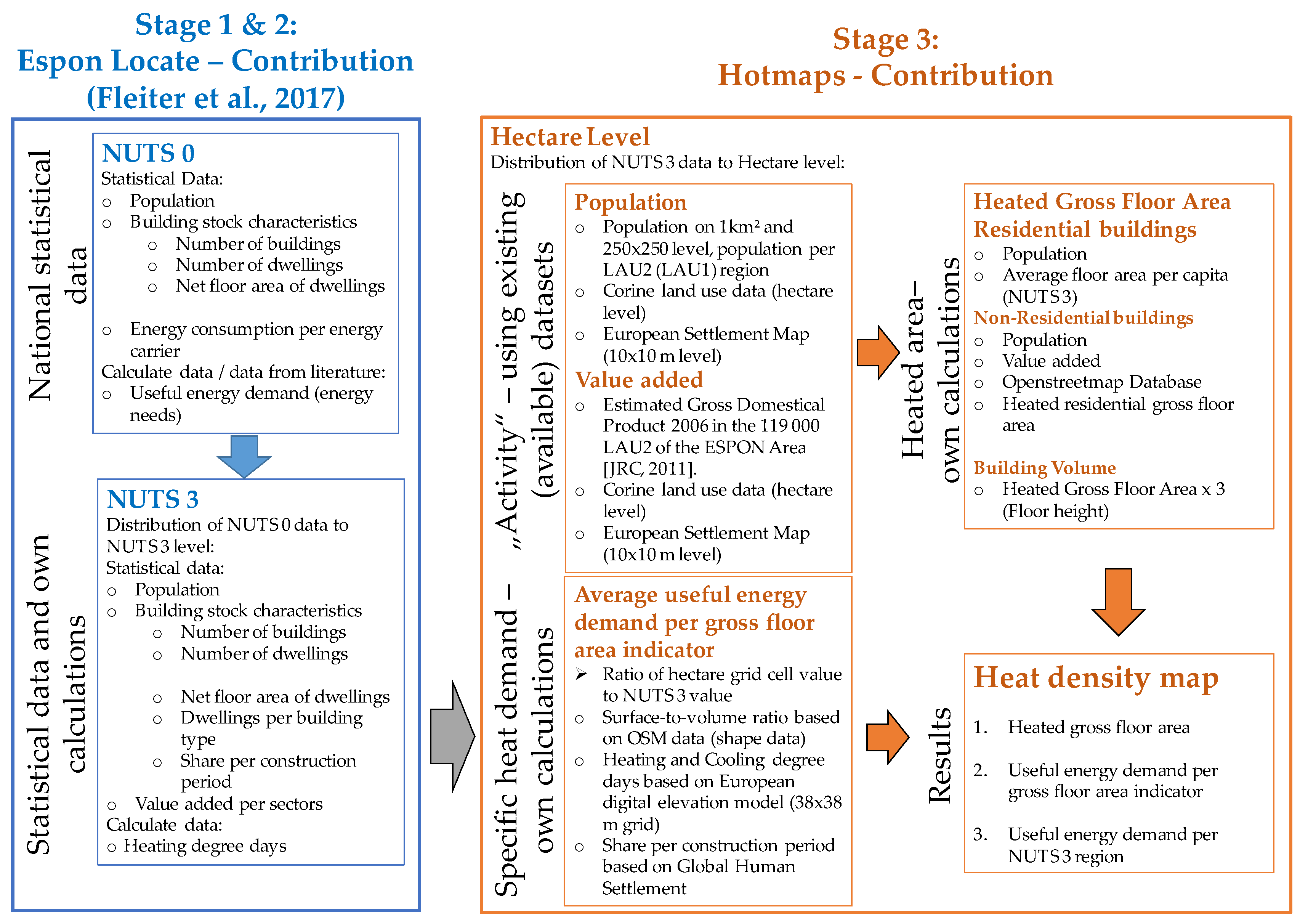
2. Materials and Methods

2.1. General Approach

The top-down heat density map developed in the Hotmaps project builds on a three-stage approach (see Figure 1). In the first stage (top-level), we derived the final energy demand (FED) and energy needs (EN) for space heating (SH) and domestic hot water preparation (DHW) based on extensive literature research for the individual countries considered in the study. These data sources include the following: energy consumption data from energy statistics (e.g., data derived from Eurostat and national energy balances [37]), statistical data on the number of buildings, households, and shares of those per construction period [38], statistical and project related data on the typical properties of different building types and construction periods per country, and average climate data for different regions. From these data we built a building dataset for each country [39], which consistently combines these different types of input data, starting with the u-values for different building components and associated typical heat transmitting areas on the one hand and, on the other, the energy consumption reported in the national energy balances for the energy services focused upon by this analysis. This step is done by applying the Invert/EE-Lab model ([40], see also [41]). The Invert/EE-Lab model is a dynamic building stock model that calculates the energy needs and final energy consumption for SH and DHW, as well as the space cooling for regions or countries based on an underlying building physics model described by national and international norms [42,43,44,45,46] alongside the energetic properties of archetype buildings and their building components, climate, and usage data [40].

In the second stage, we distributed the EN for SH and DHW from the country level (NUTS 0) to the third territorial units at the statistics level (NUTS 3) based on an approach that we developed within the study, “Territories and low-carbon economy” (ESPON Locate) [47]. At this stage, we combine several indicators to estimate the share of EN for SH and DHW for the different NUTS 3 regions within each country.

For residential buildings, we consider the following indicators. Additional information on this approach is presented in the final report of the Espon Locate project [47].

• Data provided by the European Census Hub 2011 [48]:
  • Persons (population);
  • Number of dwellings;
  • Useful floor space per dwelling;
  • Number of dwellings per period of construction;
  • Number of dwellings per type of building;
• Heating degree days (HDD) at the NUTS 2-level are based on Eurostat [49]. Within the NUTS 2 level, the HDD at the NUTS 3 level are calculated based on the average HDD (18.5/18.5) calculated from the observed daily temperatures on a 25 × 25 km grid for the period 2002–2012 (see [50]).
• The final energy demand (FED) per m² gross floor area and building types are based on the Invert/EE-Lab model results derived by Fleiter et al. [37].

The following indicators are used for non-residential buildings (only services, excluding large industrial production facilities, etc.):

• Population, HDD, EN, and FED per m² gross floor area, building type, and construction period based on the Invert/EE-Lab building stock database [48];
• The share of dwellings per construction period of apartment buildings [48];
• The total value added of the service sector [51];
• The sectoral value added (VA) to the following sectors: (a) accommodation, restaurants, stores, and warehouses; (b) other private services; and (c) public buildings, research and education, art, culture, and the health sector [51].

The third level constitutes the distribution of the NUTS 3 results at the hectare level and thus derives a heat density map. We developed an approach that correlates information from the locally built environment with its EN for SH and DHW preparation within the Hotmaps project and applied it to the EU28 countries, plus Norway, Iceland, and Switzerland. This was done by using a spatial distribution function based on similar indicators used at to transfer country data to the NUTS 3 level. This approach builds on the central idea that the EN for space heating and domestic hot water preparation correlates with the population number within a plot area, as well as its economic activity, climatic conditions, and some building properties, such as the average construction period and volume-to-surface ratios of the buildings. The final energy consumption (delivered energy plus thermal energy provided by on-site renewable energy sources) is then calculated from the energy needs by applying the country specific national conversion factor between the energy needs and final energy consumption.

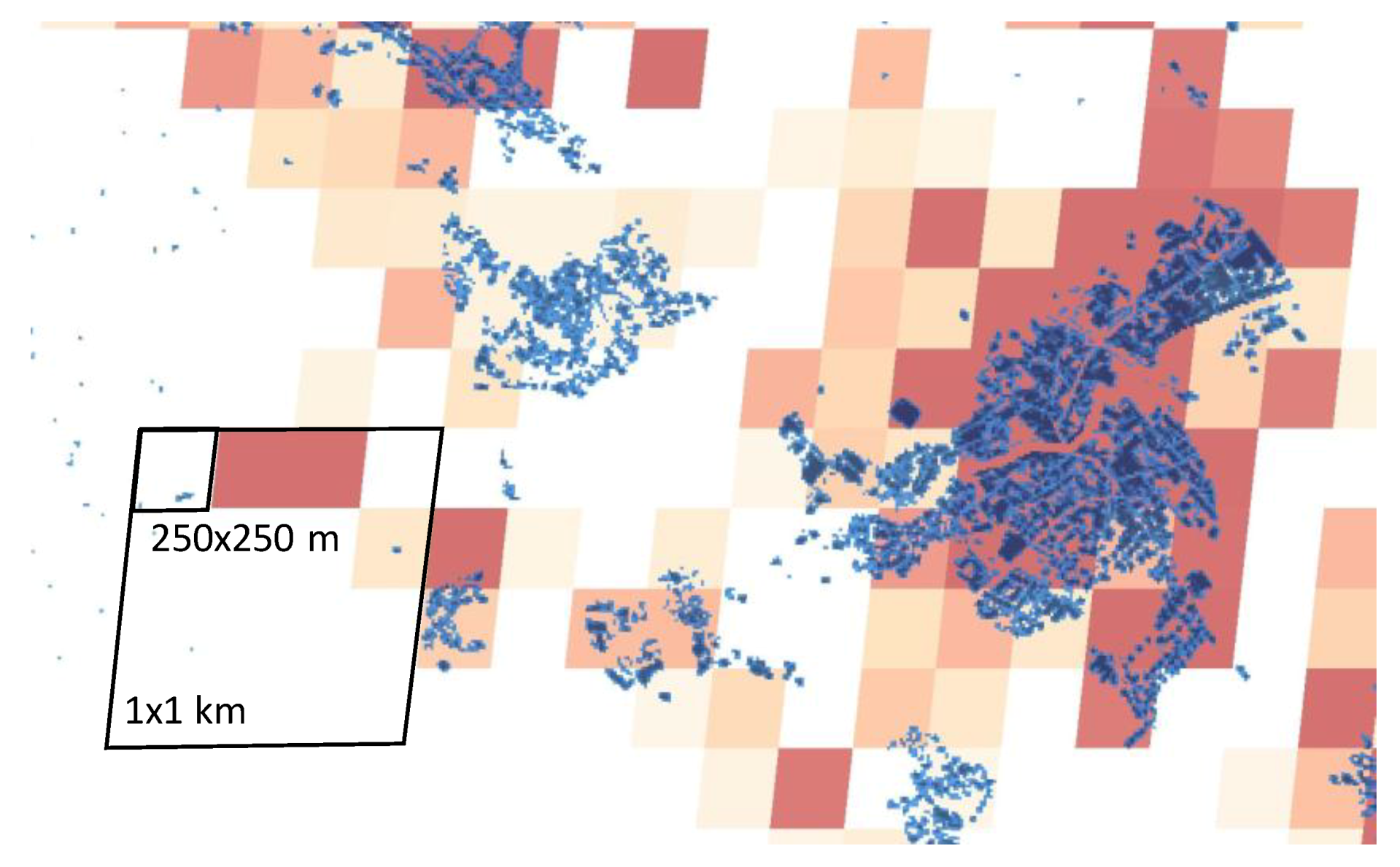
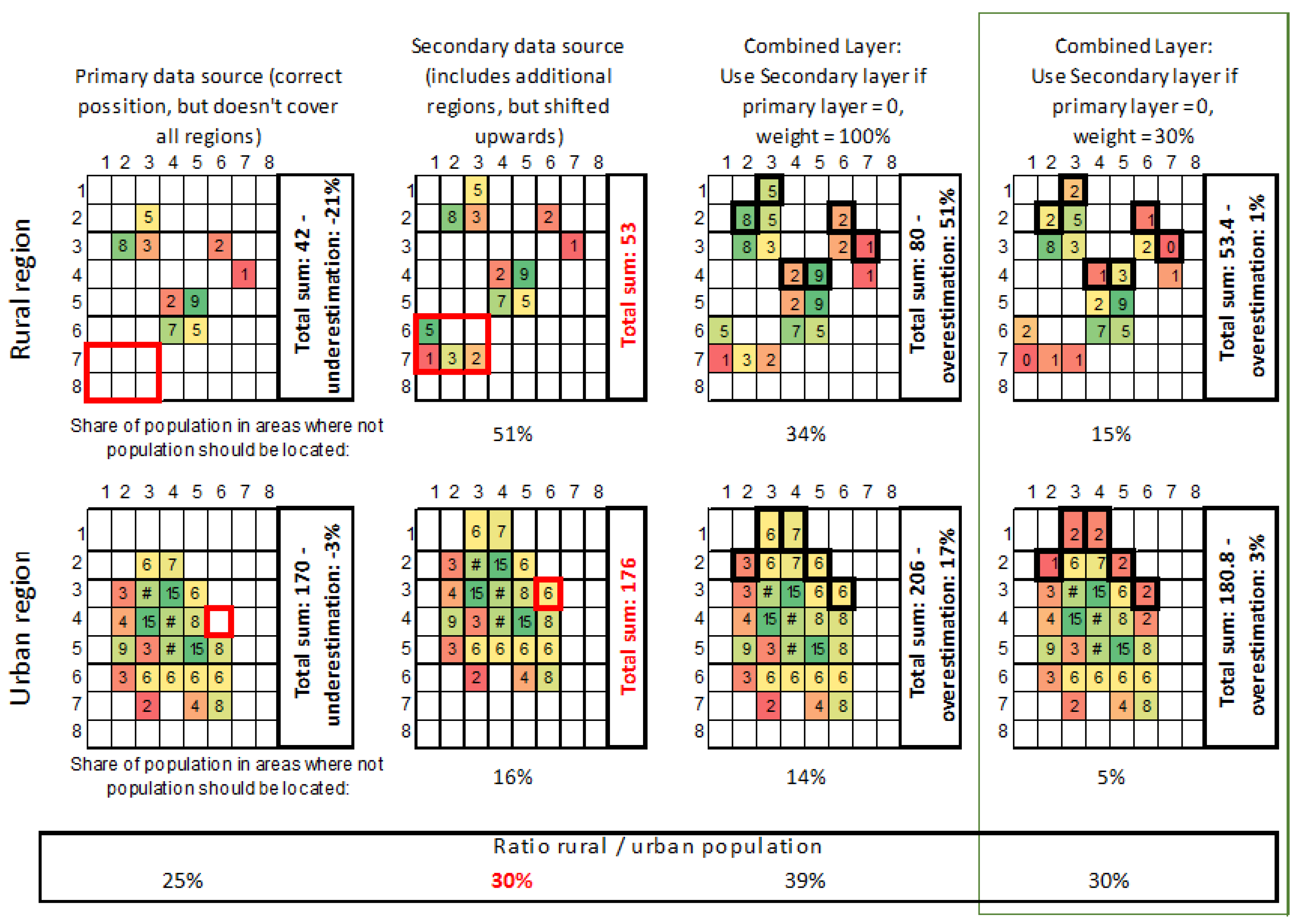
2.2. Population Distribution at the Hectare Level

Our main source for local population data is a work published by Gallego [52], where a dataset for the European population in 2006 at the level of 1 km² is given. In addition, we considered a dataset for the population in 2014 at the level of 250 × 250 m, developed by JRC [53], which is also publicly available. Although the latter source is newer, we decided to use the older population data as the primary input data source for the population distribution because a comparison of the population based on these data sources and data from the human settlement project (i.e., the share of the plot area sealed by buildings at a 10 × 10 m level) [54] revealed that a significant share of the population in rural regions is distributed in areas with no buildings (see Figure 2).

An advantage of the new JRC population dataset [53] over the older dataset of Gallego [52] is that the new dataset partly covers areas that do not feature data in [52]. To combine these two datasets, we, therefore, calculated the population distribution on a 1 km² raster for Europe based on the following rules. If the primary population layer [52] does not contain data for a 1 km² grid cell, we use the data from a 1 km² grid cell layer derived from [53] as a fall-back option. An analysis of the resulting quality of the combined layer indicated that:

(a)

The combination actually adds data in areas where the primary population layer does not cover all regions;

(b)

However, it also introduces a bias towards higher populations in less densely populated areas since a (non-systematic) shift in the (1 × 1 km²) grid cells between the two population layers can be observed in many regions. That is to say, for example, data source 1 locates the population in a neighbouring cell, similar to data source 2.

Consequently, we obtain an overestimation of the population in rural areas when we distribute the population of the NUTS 3/ local administrative units (LAU) regions at the hectare level. To reduce this undesired effect, we give the population of the JRC layer a weight factor of 30% (by multiplying the population data with a factor of 0.3). We have chosen this value by assessing the results that we derived for different weighting factors (in the range of 10–100%) for different regions (see Figure 3). This value, we believe, offers a good compromise that balances the two effects that accompany the data: first, the described effect of overestimating the population in rural areas and secondly, the underestimation of population in areas not covered by Gallego. We, however, have not performed any systematic analysis on the optimal level for the applied weighting factor.

Within the 1 km² grid cells, we distributed the population by considering the land usage type at the hectare level using the Corine land cover data [55] and the European Settlement Map layer [54], which depicts the share of the surface that is sealed by buildings on a 10 × 10 m grid. After distributing the population at the hectare level, we sum up the population for the local administrative units (LAU). This is done for the ~115 thousand regions (Eurostat [56], using the LAU 2, except for Greece and Denmark, where we used LAU 1, since the Census 2011 was performed at the LAU 1 level only). We then compared the population values with the population data in the local administrative units stated in the statistical data sources of Eurostat [48,57] and JRC [58]. To reduce the deviations, we then adjusted the population distribution to determine a compromise between the populations at the square kilometre level [52,53], the population per LAU region, and the upper limit for the population density per hectare. For this upper limit, we analysed the distribution of the indicator: the population per hectare divided by the population in the corresponding 1 × 1 km grid cell. For this analysis, we calculated the ratio between the population per hectare and the average population within the same square kilometre grid for each hectare cell. We than clustered the outcome by the population densities at the 1 km² grid level and removed all data points that did not exceed the average results for the density by a factor of 2. For the remaining data points, we calculated 95% and 99% for different population densities and defined an upper limit for the population at the hectare level (Figure 4), which is in the range of the 95–99% percentiles. The corresponding figure is read as follows: If 10 people live within a certain 1 × 1 km grid cell, then the population of each hectare cell within this 1 × 1 km² grid cell must not exceed ~5 inhabitants (50% of the total population of that square kilometre). If a 1 × 1 km² grid cell is populated by 10,000 people, the upper limit for inhabitants per hectare within that square kilometre must not exceed ~700 people (7%), and, for a population of 100,000 people per km², the upper limit for the population per hectare in that area is 2000 people (2%).

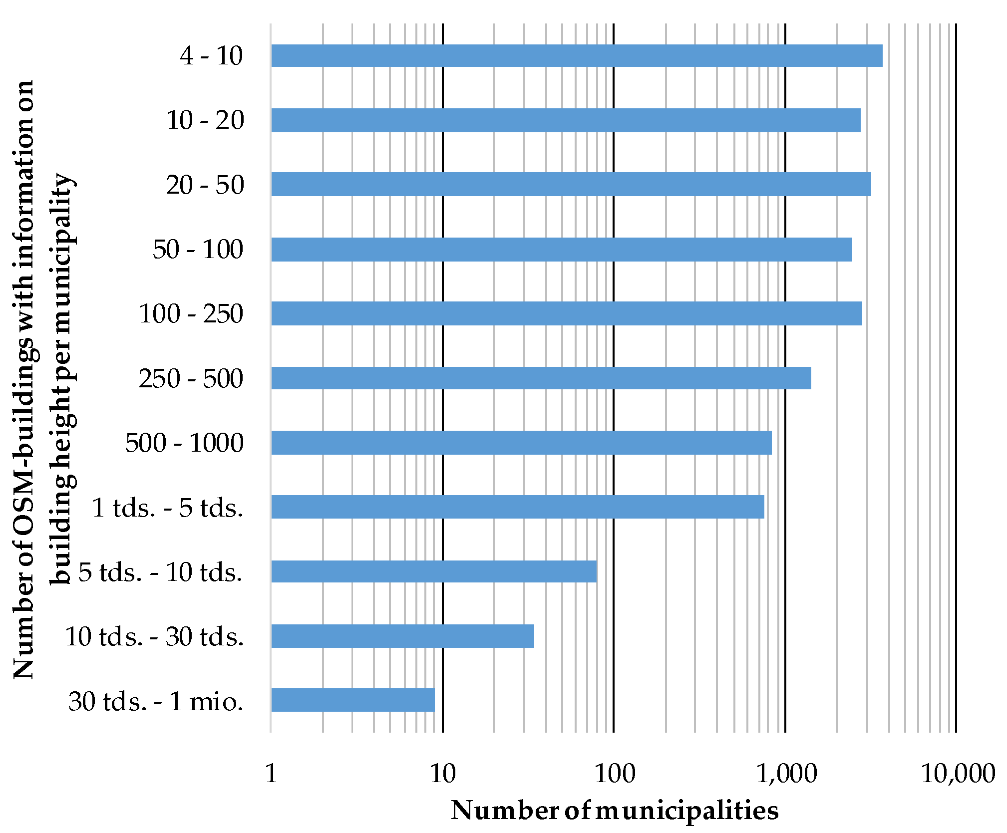
2.3. Gross Floor Area of Buildings at the Hectare Level

Our methodology estimates the heated gross floor area of buildings at the hectare level based on two independent approaches. The first approach, which we call the “population-based” approach, builds on the population grid at the hectare level and estimates the gross floor area by multiplying the population on the hectare level with the average gross floor area per person in the corresponding NUTS 3 region. We derived this indicator from the data provided by the European Census Hub [48] for most European NUTS3 regions, namely the average floor area per dwelling and the average persons per household. This approach delivers reasonable results for the residential building stock. However, its predictive quality is poor in areas with a high share of non-residential buildings. To overcome this problem, we developed a second independent layer for the gross floor area of buildings.

The second approach derives the heated gross floor area by considering the building footprints and the estimated number of floors per buildings. We extracted the building footprints from the European Settlement Map [54] and data from the building layer of the OpenStreetMap (OSM) database [59]. The European Settlement layer contains the share of plot area that is sealed by buildings on a 10 × 10 m grid, while the OSM database contains the buildings as 2-dimensional vector data.

To calculate the gross floor area from the building’s footprint, we required information on the building height or number of floors. In order to obtain estimates for these parameters, we developed a building height model that estimates the average building height from the footprint of the buildings using the OSM-building data. The developed approach applies a generic building height model (Figure 5), which is refined by the average regional (municipality-specific) building height-to-building footprint derived from buildings whose building height information is stored in the OSM database (~5 Mil. buildings spread over Europe).

As can be seen from Figure 5, the generic model for the number of floors matches well for buildings with a 60 to 1000 m² building footprint. It is assumed that buildings with footprints below 30 m² are mostly unheated (no floors) and are partially unheated if the footprint is between 30–45 m² (number of floors of 0.5). For buildings larger than 1000 m², the OSM-data show a further increase in the building height, while we, in contrast, keep the height constant until reaching buildings of 2500 m² and gradually reduce the number of floors to three for buildings with a footprint of 10,000 m² or more. The underlying reason for this method is as follows. The OSM-data mostly contain the building height, while the number of floors is calculated by us based on a constant floor height of 3 m (including structural elements). Based on personal experience, we believe that the ceiling height of very large buildings (industrial production halls, shopping centres, etc.) will be higher compared to smaller buildings and that the number of floors of such facilities rarely exceeds four. In the case of the OSM-data point for the largest building cluster (i.e., buildings with a footprint of more than 2500 m² (~20,000 buildings with a median footprint of about 6500 m²)), the average floor height would correspond to about 5 m if we consider an average number of floors as 3.5. To us, this number appears plausible.

In order to estimate the average relationship between the building footprint and the building height, we calculated the number of floors for different building footprint sizes per municipality (~18,000 municipalities out of ~115,000 in the covered region, see Figure 6).

While each individual building from the OSM database with some information on their building height is given a weight of 1, the generic model for the number of floors is given a weight of 20. The resulting relationship between the footprint and number of floors for 150 randomly chosen municipalities (for which building height data are available) is shown in Figure 7.

In the next step, we compare the gross floor areas derived from the OSM data with those from the population-based approach. If the outcome of the OSM-based approach is lower, then we scale-up the OSM data accordingly so that they match the outcome of the population-based approach. This is done up to a factor of four. If the gross floor area per inhabitant in a hectare cell is less than 15 m² according to the OSM-based data, then the OSM-quality indicator, which estimates the completeness of the OSM data (see Figure 8), is reduced. This process leads to a lower weight of the OSM-based heated floor area data in the final calculation of the heated gross floor area (see

Table 1. Weighting of the population and value added (VA) based approach versus the OSM based approach for areas in different Corine land cover classes used to calculate the heated gross floor area at the hectare level.

Corine Land Cover Class	Residential Gross Floor Area		Non-Residential Gross Floor Area
	Weighting Factors * for Data from Approach Based on …
	Population Data wpop	OSM Data wOSM	Population & Value Added Data wpop	OSM Data wOSM
1: Continuous urban fabric	1	0.05	1	0.05
2: Discontinuous urban fabric	0.9	0.05	0.9	0.05
3: Industrial or commercial units	0.7	0.05	0.7	0.05
10: Green urban areas	0.1	0.05	0.1	0.05
11: Sport and leisure facilities	0.1	0.05	0.1	0.05
18: Pastures	0.5	0.05	0.5	0.05
20: Complex cultivation pattern	0.5	0.05	0.5	0.05
21: Land principally occupied by agriculture	0.5	0.05	0.5	0.05
Other classes	0.015	0.05	0.015	0.05

* The actual weighting factor is calculated, e.g., as w_pop/(w_pop + w_OSM).

).

Finally, the heated gross floor areas of the residential and non-residential buildings are calculated by combining the results of both methods. For residential buildings, we used a weight factor between 0.015 and 1 using the population-based approach (depending on the Corine land cover class (see Table 1), while the OSM-based approach is given a weight of 5%, if there is no indication that the OSM does not fully cover the given grid cell.

To estimate the heated floor area of non-residential buildings, we use (a) the value added per LAU region [45] instead of the residential floor area per inhabitant indicator and (b) the OSM-based approach. We calculate the non-residential heated gross floor area by subtracting the residential gross floor area from the calculated gross floor area using the OSM-building information. Compared to the residential gross floor area, we used a comparatively higher weight in the OSM-approach for non-residential buildings since the quality of the OSM data (degree of completeness) is estimated to be high. Based on own estimations, Table 1 depicts the detailed set of weighting factors that we used in our approach for different Corine land cover classes. These weighting factors are taken for areas where the OSM data quality is estimated to be high. If the data quality of the OSM data is considered to be low (see Figure 8), then the weight of the OSM approach is reduced accordingly.

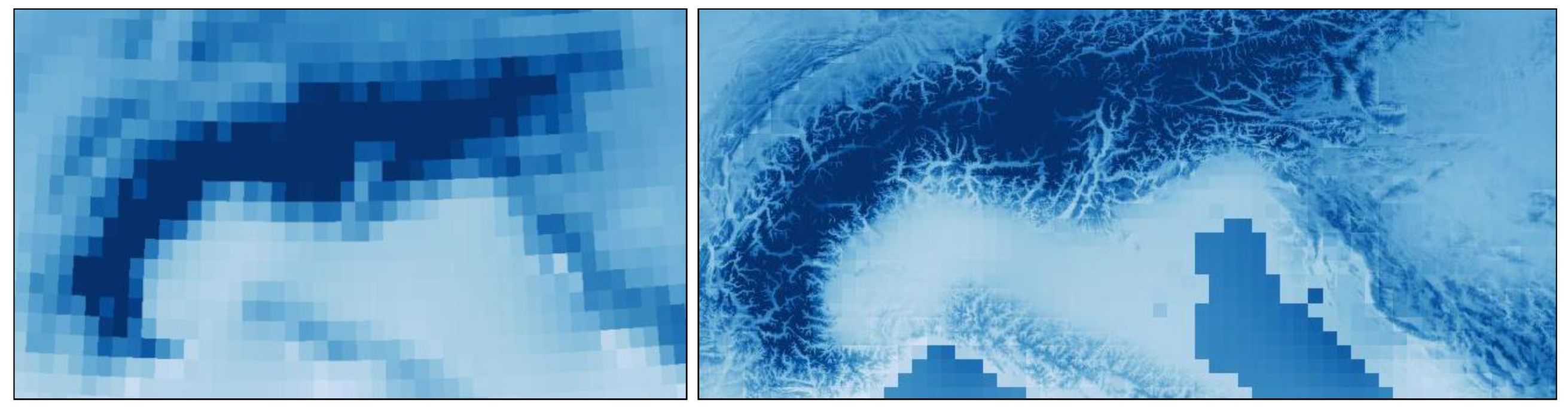
2.4. Heating Degree Days at the Hectare Level

The starting point for the calculation of the local heating degree days is the observed average daily temperatures on the 25 × 25 km raster [50] for the period from 2002 to 2012. With a resolution of more than 600 km² per raster cell, this layer is too coarse to derive meaningful local heating degree days, as shown in Figure 9 (left figure) for the Alpine region, North Italy, and Croatia. To refine these data, we included in the calculation information on the local elevation using the digital elevation model over Europe (EU-DEM) layer at the 30 × 30 m grid level [60] and applied a temperature lapse rate of 6.5 °C per 1000 m elevation gain according to the specifications of the International Standard Atmosphere model [61] (see Figure 9, right).

The energy needs for space heating (SH) on a local level are corrected by applying the ratio between the calculated site’s specific HDD and the HDD at the NUTS 3 level using an elasticity of 0.5. We purposefully corrected the energy needs for the local climate conservatively, as we tried carefully to avoid “overshooting” our corrections and instead preferred results that are “too” uniform for different areas. With such low elasticity, we also covered the (plausible) assumption that buildings in colder areas (e.g., those at higher elevations), in general, might already have higher energy performance than similar buildings in warmer (lower) areas, even if they have to fulfil the same energy performance standards.

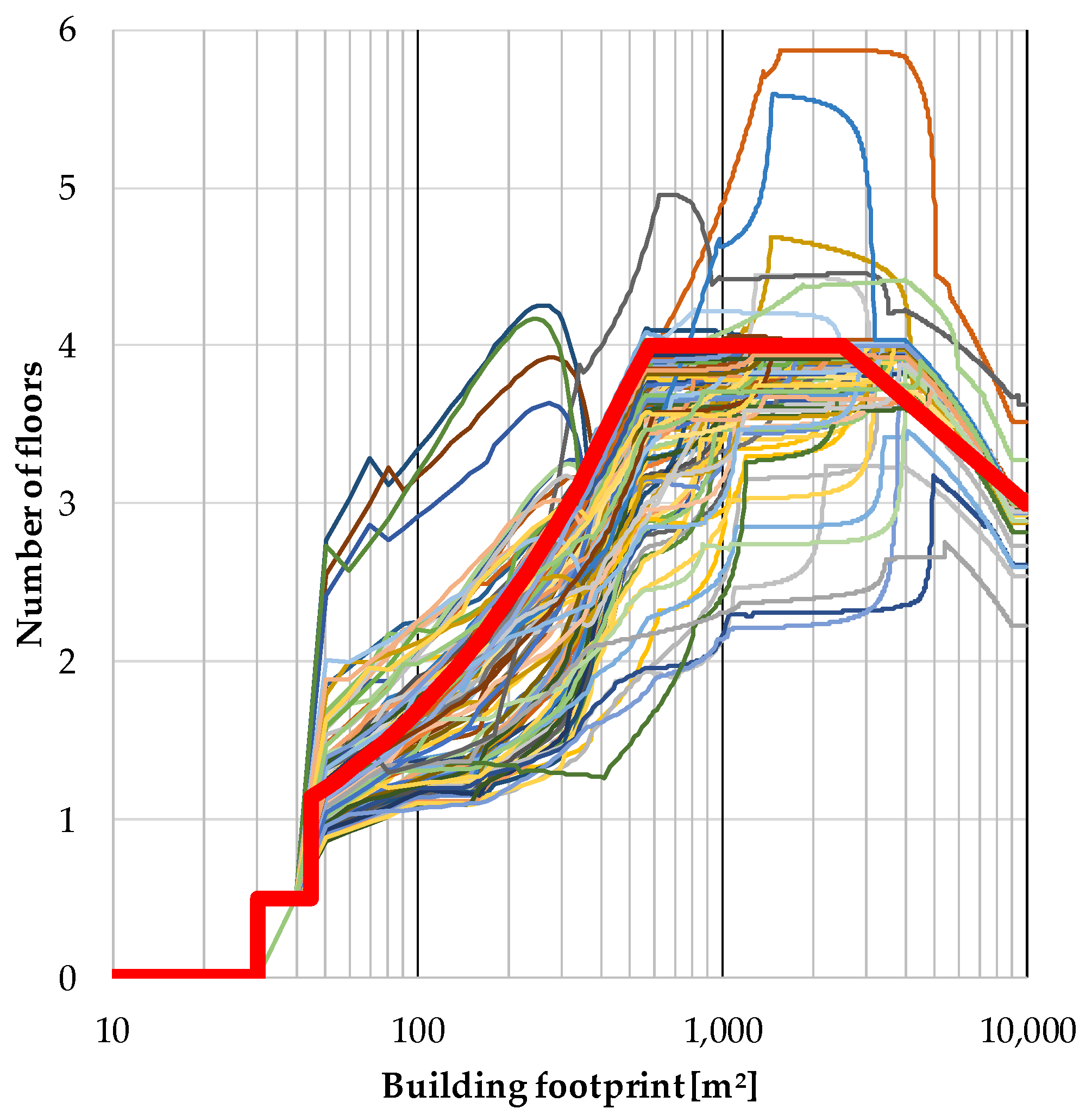
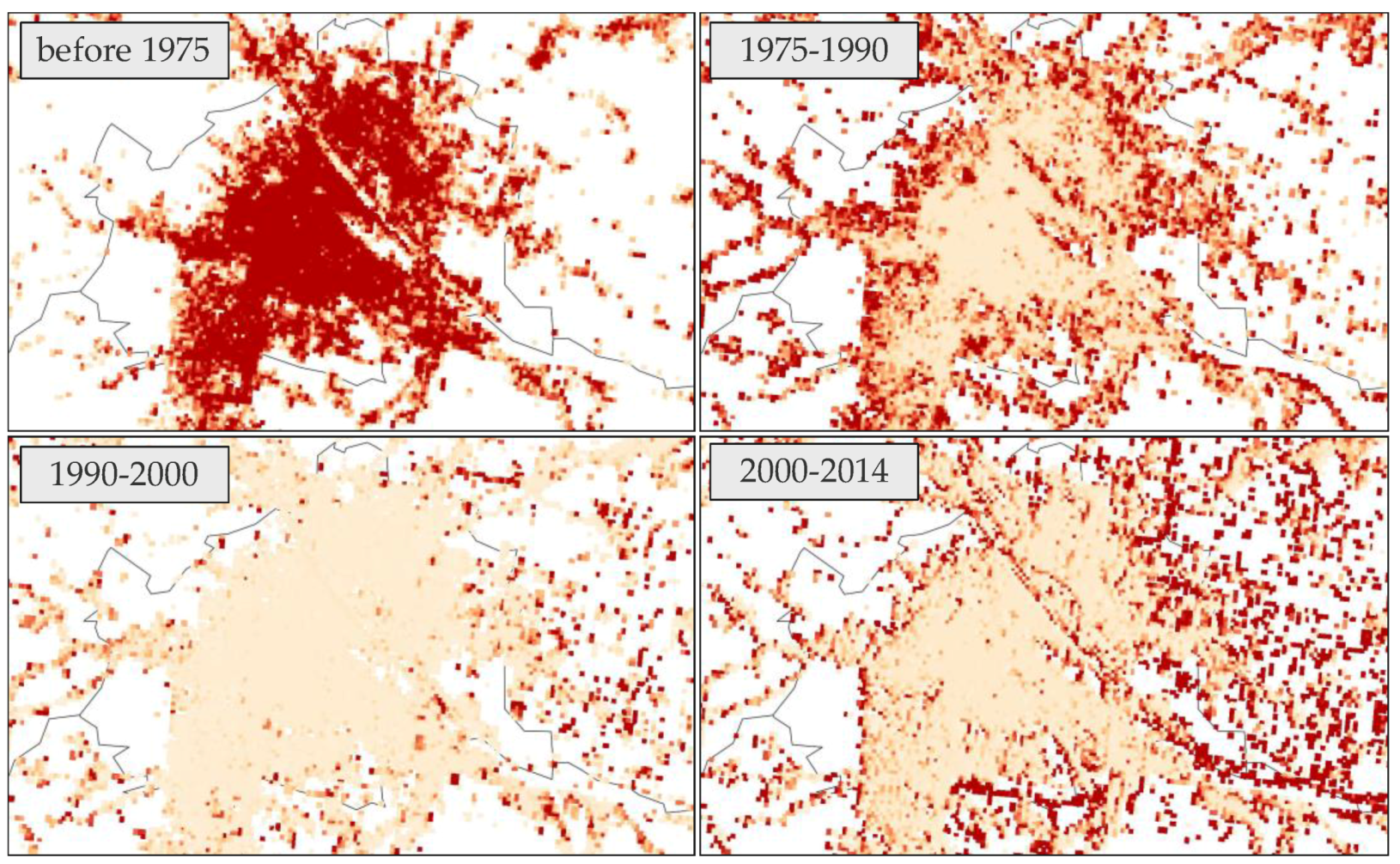
2.5. Surface-To-Volume Ratio of Buildings and Historical Construction Periods

In order to calculate the spatial distribution of EN and the final energy demand (FED) for SH from the heated floor area, we furthermore considered the surface-to-volume ratio of buildings and the share of buildings per construction periods. To obtain data on the surface-to-volume ratio, we built on the data from the OSM building layer: the building footprint (area and perimeter) and the estimated building height. For the share of buildings per construction period, we extracted information on the soil sealing data provided by the Global Human Settlement project [53] for 1975, 1990, 2000, and 2014 on a 38 × 38 m grid. Besides comparing the soil sealing ratio per grid cell for the time slots, we tried to correct the data for the soil sealed by other elements, such as roads, by considering the current share of soil sealed by buildings against the total share of sealed soil per grid cell (at the hectare level). We also generically considered building demolition. For the period after 2000, we considered an annual demolition rate of 0.2% for buildings constructed before 1975 and 0.1% for buildings constructed between 1975–1990. Thus, we assume that the stock of buildings constructed before 1975 is only 97% of that shown in the soil sealing map due to building demolitions between 2000 and 2014. Furthermore, we assume that at least 0.75% of the soil sealing share in each period (1975/1990/2000/2014) must stem from buildings constructed in the latest construction period. This means that if the soil sealing is 40% for a given grid cell in 1990, then the share of soil sealed by buildings constructed between 1975 to 1990 must be at least 40% × 0.75% = 0.3%. If the soil sealing map of 1975 already depicts soil sealing of 40%, we reduce that value by 0.3% and add that value to the construction period from 1975 to 1990. As an example, the outcome of this process is visualised in Figure 10 for the region of Vienna.

As with the local heating degree days, we tried to conservatively correct the energy needs for the surface-to-volume ratio and construction periods. Again, we manually performed checks for different regions to indicate that the outcomes are plausible on a general level. We needed to remain cautious of the significant uncertainties of this methodology. Therefore, we gave these two factors a rather low weight and considered an elasticity of only 33% for the surface-to-volume ratio. To buildings constructed after 2000, we assigned a specific EN of 80%, and to buildings constructed before 1990, we assigned an EN of 125%, which was compared to the specific energy needs per building (for buildings constructed from 1990 to 2000).

2.6. Comparison of the Resulting Data with Data from Other Sources

In order to better understand the characteristics and quality of the developed gross floor area (GFA) density and heat demand (HD) density layers, we compared these with data from other sources. We did this at the following regional levels:

• For several NUTS 3 regions in Austria and Switzerland, a comparison of the overall gross floor area (GFA) of residential and service buildings and the respective final energy demand (FED) has been performed over the course of the project ESPON locate. The results can be found in the following report [47].
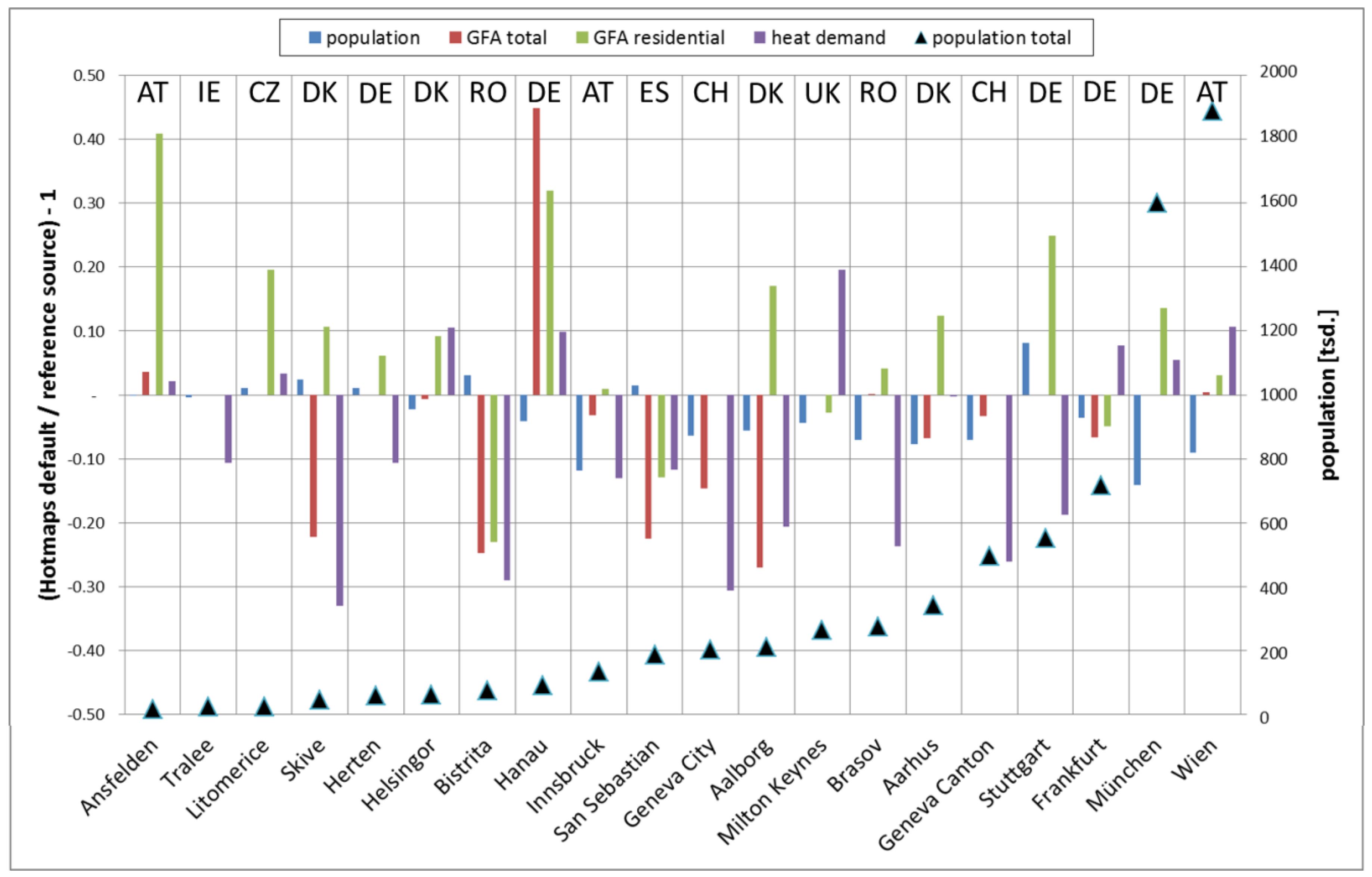
• For several LAU and NUTS 3 regions across Europe, we collected and compared the following data: number of inhabitants, GFA of residential buildings, GFA of service buildings, and FED for space heating and hot water preparation in residential and service buildings. We collected these data from local statistics on buildings and energy use and from reports of other projects (see

  Table 2. Data sources of the reference values for comparison at the LAU/NUTS level.

  Location	Country	Data Sources
  Ansfelden	Austria	[64]
  Tralee	Ireland	[65]
  Litomerice	Czech Republic	[66]
  Skive	Denmark	[67]
  Herten	Germany	[68]
  Helsingor	Denmark	[69]
  Bistrita	Romania	[70,71]
  Hanau	Germany	[72]
  Innsbruck	Austria	[73,74]
  San Sebastian	Spain	[75,76]
  Geneva City	Switzerland	[77]
  Aalborg	Denmark	[67]
  Milton Keynes	United Kingdom	[78]
  Brasov	Romania	[79]
  Aarhus	Denmark	[80,81]
  Geneva Canton	Switzerland	[77]
  Stuttgart	Germany	[82,83]
  Frankfurt	Germany	[84,85]
  München	Germany	[86]
  Wien	Austria	[87,88]

  ).
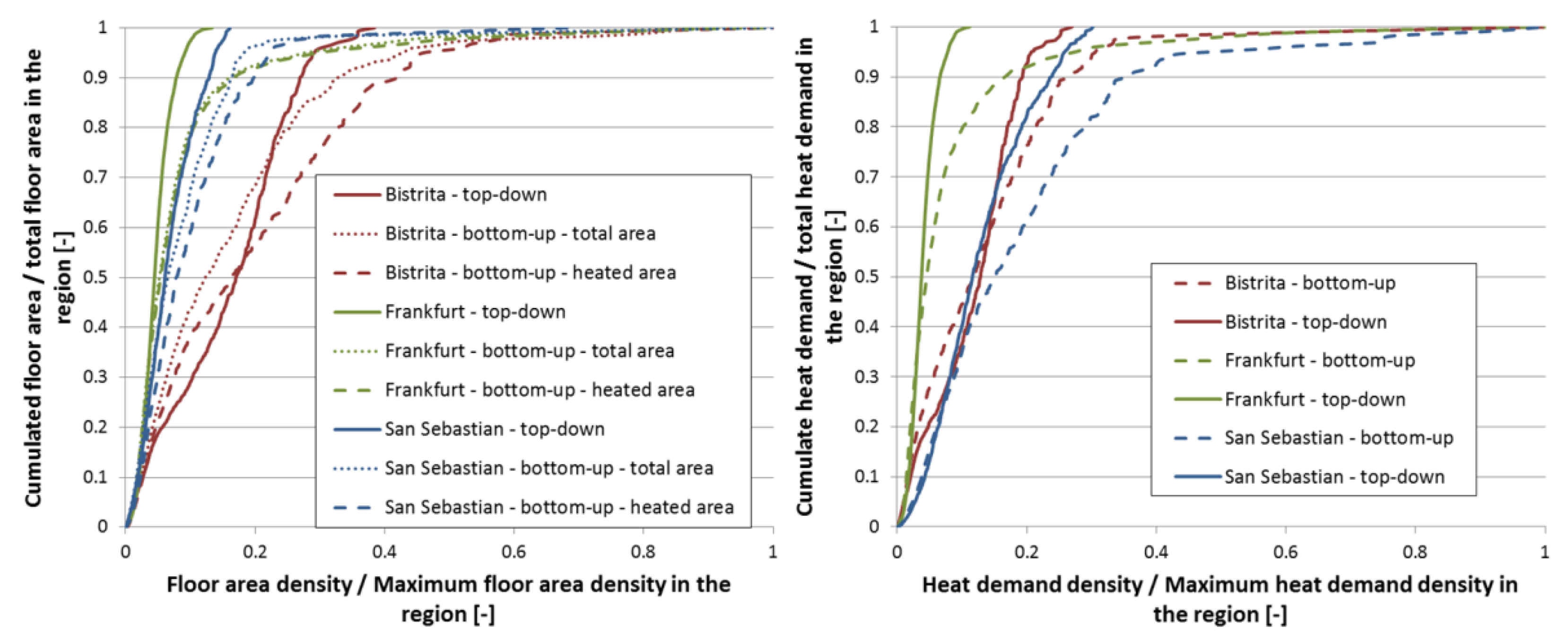
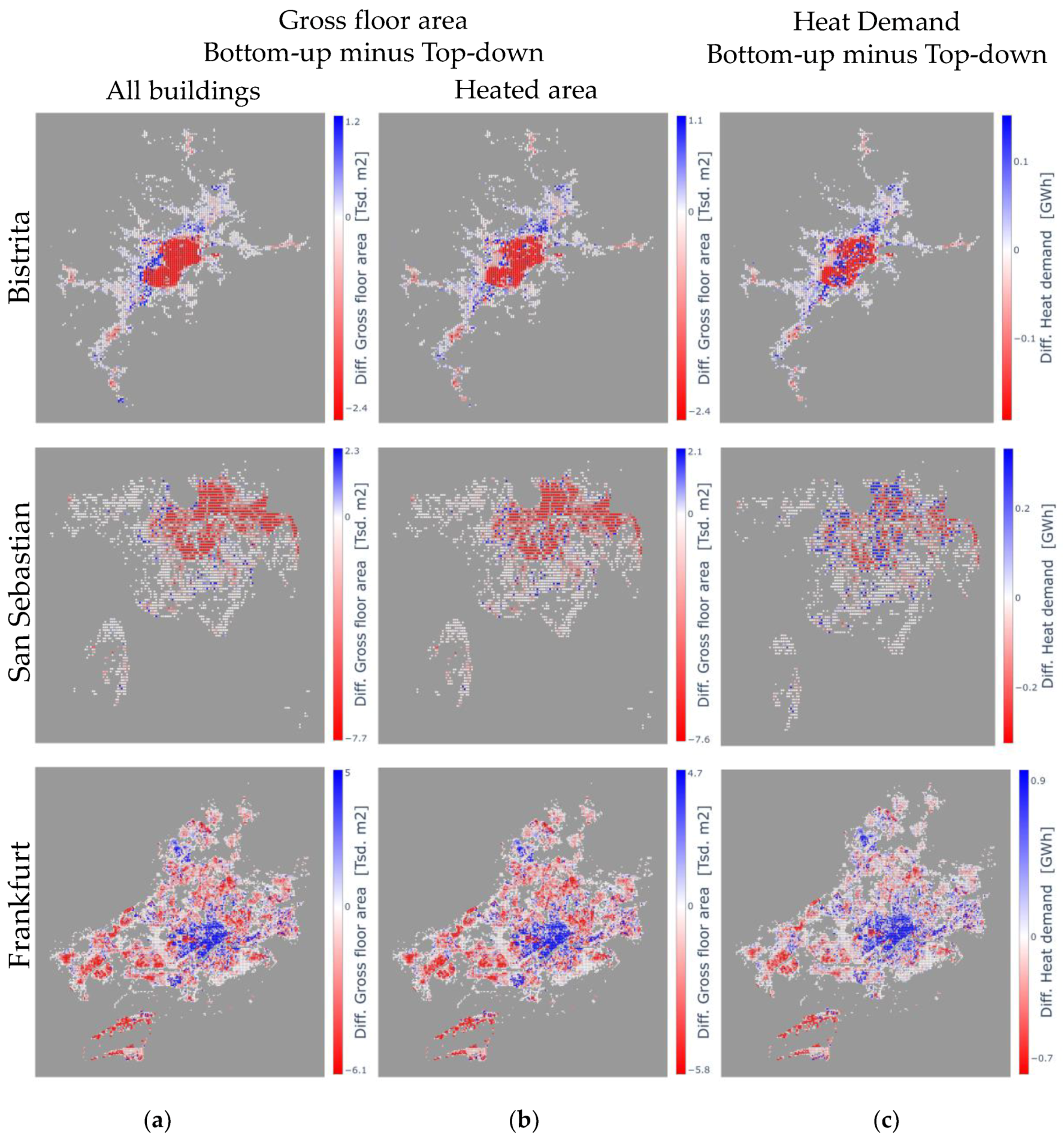
• For three cities in Europe, we compared the developed GFA and the HD density maps with maps developed on the basis of building stock data from the city administrations. Then, we compared the values of both maps at the level of 100 × 100 m raster elements. These maps were developed according to the following methodology:

  ○

  The basis for the bottom-up calculation of the GFA and the EN of the buildings in the three cities are shape files of the buildings containing the following information: shape and location of the building footprint, number of floors, building height and type, as well as age of the building. If data for certain buildings were missing, we filled these gaps using the average values of the other buildings with similar characteristics in the database.

  ○

  In the second step, we joined these building stock data with data on specific EN values for space heating and for hot water generation from the Invert/EE-Lab model [40]. With this model, we calculated these values for typical buildings in the countries according to the type and construction period of the buildings. The resulting values applied to the overall building stock in the countries match the national energy balances. In joining the values with the building stock databases of the cities, we performed climate correction from the average heating degree days (HDD) in the countries to the HDD in the cities. For this, we used the HDD data from the Hotmaps database (see Figure 9, available at [62]).

For the comparison, we used data from published and unpublished sources. At the NUTS 3 or LAU level for several locations, data can be found in the published literature. However, for many regions and municipalities, data on the energy demands of space heating and hot water generation, or on the number of buildings, are only available in unpublished databases or reports. Because public authorities usually do not publish their building inventories, for our comparison at the hectare level, we were only able to use unpublished data.

3. Results

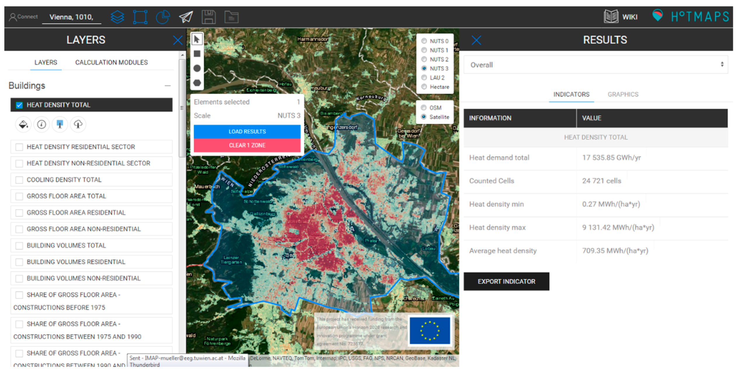
3.1. Resulting Maps and Data

The developed raster files for gross floor area and heat demand for space heating and hot water preparation in residential and non-residential buildings are integrated into the Hotmaps database and toolbox and are accessible on their respective webpages [63]. On the website, these data can be visualised and analysed for selected locations and can be used in the different integrated calculation modules. Figure 11 shows a screenshot of the heat demand density total layer and the provided indicators for the NUTS 3 region of Vienna.

The layers are also available for download from the Hotmaps database and toolbox or directly from a GitHub repository. The corresponding links are given in the supplementary materials section at the end of the manuscript.

3.2. Comparison of Results with Data from Other Sources at the NUTS 3, LAU 1, and LAU 2 Levels

To understand the quality of the developed gross floor area (GFA) and heat demand (HD) data, we first compare these at the levels of the NUTS 3, LAU 1 (local administrative units), and LAU 2 regions with data from other sources. We collected data on population, residential GFA, total GFA, and HD for space heating and hot water generation in residential and tertiary buildings for 20 different regions. Table 2 lists the data sources we used, and Figure 12 shows the results of this comparison.

This comparison of the developed data and other sources for the 20 selected regions shows an average difference of 12% in the mean values among the absolute values, with a standard deviation of 10% and a deviation of 8% for the median values. However, for some values, we found nearly no difference between the developed and other data. Some values show remarkable differences up to 45%. The values for the population and total GFA seem to better match the developed data and other sources, whereas residential GFA and HD show greater differences. Residential GFA, on average, is 9% higher in the developed data, and the HD, on average, is 8% lower. Both show a standard deviation of 16%. For regions with higher numbers of population, the differences seem to be lower. However, these statistics on the difference between the developed data and other data have a high uncertainty mainly due to the limited number of regions under comparison and the limited certainty of data from other sources. We discuss these uncertainties in Section 4.2.

3.3. Comparison of the Results with Data from Other Sources at the Hectare Level

For the cities of Bistrita, San Sebastian, and Frankfurt, we compared the developed gross floor area (GFA) and heat demand (HD) density maps (top-down) with maps developed from municipal building stock databases (bottom-up). Both types of maps were created with the same projection and raster size. For the comparison, we scaled the values in each hectare element of the top-down maps using the following ratio: the sum of the values of all hectare elements in the bottom-up map divided by the sum of values of all hectare elements in the top-down map. This allows us to focus on the difference of the distribution of the GFA and HD in the territories between the top-down and the bottom-up maps. For HD, we compare two maps: the top-down map and the bottom-up map. For GFA, we compare three maps: the top-down map, the bottom-up map of the GFA for all buildings in the region, and the bottom-up map showing only the heated GFA (HA) in residential and tertiary buildings.

In the first step, we compared the distribution of the GFA and HD over the GFA and HD density in the top-down and bottom-up maps. Figure 13 presents these distributions, showing the cumulated GFA and HD values for all hectare elements, from the elements with low density to the elements with high density. In order to compare the distributions for the three cities, we normalized both axes.

The figures show that, in the top-down maps, the GFA and the HD are distributed over a smaller range of GFA and HD density compared to the bottom-up maps. The maximum density in the bottom-up maps is remarkably higher than the maximum density in the top-down maps: e.g., in Frankfurt, in the top-down map, the highest GFA density is only 13% of the highest GFA density in the bottom-up map; for HD in Frankfurt, the GFA density is even lower at 11%. This is the same for all analysed cities but with a lower difference between the maximum values. Furthermore, the GFA and the HD are more evenly distributed in the top-down maps than in the bottom-up maps. The strong increase of density for the 5–10% GFA and HD in the areas of highest density visible in the bottom-up maps is remarkably underestimated in the top-down maps. Due to the fact that these characteristics can be found for all comparisons between the top-down and bottom-up groups, this seems like a systematic difference between the top-down and bottom-up results.

The figure also shows that the form of the distribution of the GFA and HD over the GFA and HD density is similar in the bottom-up and top-down maps. That is, the slope of the distribution curve for Frankfurt is steeper than that for San Sebastian, and the slope of the curve for San Sebastian is steeper than that for Bistrita. This is the same for both the bottom-up and top-down maps, as well as for the GFA and HD comparison. Finally, we also in the comparison of the GFA maps that the bottom-up maps showing only the heated area (HA) match better with the top-down maps for the three cities than with the bottom-up maps showing the entire GFA for all buildings in the region. This result seems logical, as the top-down maps reflect the heated area only.

For the second analysis, we compared the values from the top-down and bottom-up maps for each hectare element. Figure 14 shows the difference between the bottom-up and the top-down value in each hectare element for the three cities. In this way, the following maps are compared: (a) a top-down GFA map reflecting the heated area (HA) in the region, with the bottom-up GFA map containing all buildings in the region (including industrial and non-energy relevant buildings); (b) a top-down GFA map with the bottom-up HA map only containing the HA of the residential and tertiary buildings; and (c) a top-down HD map with a bottom-up HD map. For this comparison, the top-down values have been scaled so that the overall GFA, heated area, and HD in the area are the same. In the figure, each hectare cell of the selected municipality is represented by a single dot. Blue dots indicate that the Hotmaps’ top-down data distribute a lower share of energy or gross floor area to a specific hectare cell then the bottom-data distribute. The hectare cells are shown in red dots if the bottom-up maps allocate a lower share.

4. Discussion

In this paper, we explained how we developed a gross floor area (GFA) density map and a heat demand (HD) density map at the level of 100 m × 100 m for the entire EU 28 (+ Norway, Iceland, and Switzerland) within the Hotmaps project. We also showed a comparison of the developed maps at the NUTS 3, LAU, and hectare levels with data and maps (developed) from other sources. In the following, we discuss the limitations of available data for the exercise and their effects on the results, as well as the uncertainty in the comparison of the results with data from other sources.

4.1. Limitations of the Data

The presented datasets and maps build on a statistical approach. This approach limits the accurateness of the data, as site specific or local conditions are not taken into account. Considering the input data, we believe that the population data are accurate up to a level between 250 × 250 m and 500 × 500 m. However, we must acknowledge that the input data are, on average, about 10 years old. In addition, the data are consistent with statistical data at the municipal level; given the limitation that statistical population data on LAU regions are not available for all census years and LAU regions (or contain inconsistencies), we used the average population data for the years 2008 to 2016. Checks, where we estimated the population of a given area using satellite images and estimations for the average number of persons per building, confirmed that the data are also plausible for higher resolutions.

Statistical data on the residential heated (net) floor area are available for most NUTS 3 regions. We again performed manual data quality checks, which indicated that our results are plausible at the hectare level for most regions. However, in the current dataset, we did not consider the observation that the heated area per inhabitant often decreases by increasing population density. For NUTS 3 regions with a strong urban versus rural area gradient, this might result in an overestimation of the heated residential gross floor area in urban areas. The heated gross floor area of non-residential buildings, however, remains very uncertain at the country level. Data quality checks indicate that the sum of the residential and non-residential heated gross floor area is in a plausible range. Also, the ratio between residential and non-residential gross floor area is plausible, although this indicator might not hold for grid cells, which contain few buildings. Furthermore, the comparison of regional building stock data indicates that we likely underestimated the floor area of non-residential buildings at the country level, which is an input in our model. The final energy demand for non-residential buildings, however, is in the correct order of magnitude, as well as the data for the heated gross floor area at the national level for building categories, such as offices, health and education, restaurants and hotels, retail and wholesale, and others. One possible reason for this result is that we overestimated the area-specific energy demand (e.g., due to the geometry of the buildings (small surface-to-volume ratio) and/or higher-than-estimated internal gains) or that a significant share of non-residential buildings is not fully heated (industrial production halls, warehouses, etc.). In order to systematically investigate this gap, further high-quality data on existing non-residential building stock is needed.

For the heat demand density map, we derived the local data from statistical data on energy consumption at the country level and national building stock characteristics, such as the average specific energy needs per construction period. To calculate the grid cell specific energy demand-per-floor area data, we assessed the surface-to-volume ratio of buildings based on the OpenStreetMap database, the share of floor area per construction periods, and the heating and cooling degree days. The impacts of the first two indicators are plausible but highly uncertain. We, therefore, give these indicators a low weight in our calculations. We belief that these last indicators, the heating and cooling degree days, are of higher accuracy, although we used a simple atmospheric temperature lapse rate model, which cannot account for local site-specific weather and climate conditions. Additional uncertainties exist, as we do not know if and how planers have already considered colder (or warmer) local climate conditions when the buildings were constructed in the past. Since we assume that this might be the case to some extent, we lowered the weight of the climate indicator compared to what is usually considered to be the actual thermodynamic degree of influence. Again, data quality checks indicate that our results are plausible. However, we recommend using individual data on the heated area-specific energy needs or final energy demands, whenever local data are available. Another uncertainty regarding the final energy consumption (which is not the case for the energy needs) arises from the lack of information on the applied heating systems and the corresponding efficiency. If, in a region or grid cell hiatus, biomass-based stoves are widely applied, then the final energy consumption will be higher than if electricity-based systems are commonly used, even if the actual energy needs of the buildings are identical.

4.2. Uncertainty in the Comparison of the Results with Data from Other Sources

To compare the developed maps with data and maps from other sources at different regional levels is important to understand the potential use and the credibility of the dataset. Although it was possible to find values for population, residential gross floor area (GFA), total GFA, and heat demand (HD) for 20 regions, the uncertainty in the statistics for the difference between the developed data and the data from other sources is high. There are two main reason for this uncertainty. First, the share of the regions for which we compared developed data with data from other sources on the overall territory covered in the developed data is very low. The 20 regions in the presented comparison cover 1.4% of the population of the entire analysed territory. Second, the reliability of the data from other sources is often unknown. Descriptions of the data stated in reports often lack detail to understand what exactly is being represented in the data, e.g., what type of heat demand is reflected, what types of buildings are taken into account, the year of reference, if the demand data are climate corrected, or what the regional borders of the analysis are. Therefore, no quantitative conclusions for the differences between the developed and other data at the NUTS and LAU level are possible.

We also compared the top-down developed maps with maps based on municipal building stock data (bottom-up) for three cities at the hectare level. The bottom-up maps were developed by estimating the HD via the average HD in typical buildings in the countries calibrated at the national level and climate corrected to the location of analysis. We found that the overall GFA and HD, as well as the split between residential and tertiary buildings, in the developed bottom-up maps match well with the data for buildings and the energy statistics from the cities. However, the data in the local statistics also imply uncertainty. Notably, the energy demand for space heating and hot water generation is not generally measured but developed based on the estimated shares of energy carriers used for different purposes. Bottom-up estimations, on the other hand, strongly depend on the input data—most importantly, energy demand per m², service factors, and building occupation. Furthermore, user behaviour is an important uncertainty when analysing HD at a very detailed regional level: Are people leaving houses for longer periods, are they used to having lower or higher indoor temperatures, or is a building or a flat really occupied or not?

5. Conclusions and Outlook

5.1. Conclusions

The developed GFA and HD density maps cover the entire territory of EU 28 + Norway, Iceland, and Switzerland. In addition, they are fully open source and therefore usable by everyone for every purpose. This is the first such dataset we know of.

A comparison of the developed data with data stated in other sources for selected cities and regions showed differences from very low up to 45%. The average difference of all compared values was 12% (median 8%), with a standard deviation of 10%. Differences in this range are also often experienced in comparing data from bottom-up estimations of GFA and HD based on local building stock data with values from buildings and energy statistics.

A comparison of the developed maps with maps based on municipal building stock datasets for three cities shows that, for these locations, the overall tendency of the distribution of GFA and HD over the GFA and HD density is similar in both approaches. This comparison also reveals the following systematic difference: The developed datasets seem to systematically overestimate the GFA and HD in low density areas and underestimate the GFA and HD in high density areas.

We conclude that the developed GFA and HD density maps allow a first analysis of GFA and HD distribution in all locations in Europe. Also, they can be used to identify areas that might be suitable for district heating. Especially for locations in Europe where detailed GFA and HD density maps are not available, the developed maps provide valuable data for initial and quick analyses. For the detailed planning of supply infrastructure, however, more detailed data from the local level should be used.

5.2. Outlook

Although the approach of developing heat density maps is not entirely new, and despite the achieved progress regarding the transparency, accessibility, and quality of the data presented in this paper, there is still a considerable need to enhance the work on heat density maps.

In the course of the Hotmaps project, the representatives of additional follower areas—beyond the cases presented above—will use the Hotmaps toolbox (www.hotmaps.eu). The creation of detailed, bottom-up heat density maps will provide the grounds for more data to be compared with the EU-28 default data map presented in this paper. The authors intend to use this process to continuously develop further calibration, a better understanding of possible deviations and biases, and regularly update the database via the toolbox and on the mentioned Git-Repository. This model, which creates the described heat density maps, will be published as open source at the end of the Hotmaps project; until then, the model is available on request.

High quality data on heating and cooling energy demands and consumption for entire regions or areas are rare and usually subject to substantial uncertainty. Thus, reference values for the plausibility checks of heat density maps are also rare and partly uncertain. In addition, even the assessment of the reliability of a source is often difficult since geographic system boundaries are not always clear, and the definitions, and indicators are often not fully documented. Thus, the improvement of data availability, reliability, documentation, and know-how on the municipal, regional, national, and European levels regarding energy demands and, in particular, heating and cooling, should be given higher priority. On the municipal level, this prioritization should also be integrated in the process of establishing strategic heating and cooling planning and mapping processes. We are convinced that a better data foundation and correspondingly trained persons are essential preconditions for more effective planning and mapping processes and thus a decarbonisation of the heating and cooling sector.

Cooling density maps have also been developed by the authors in the frame of the project Hotmaps. Due to the restricted space in this paper, we decided to limit the scope to heating only. The elaboration of cooling density maps has led to other types of uncertainties and issues that need be further analysed in future research work.

The validation and subsequent reliability of the heat density maps could be further improved by integrating other data sources. This refers, for example, to the data from the EPC databases. The project Enerfund (http://enerfund.eu/) has provided a rich map of EPC data, at least for some countries. Another important source and step to improve the quality of heat density maps is using real and measured energy consumption data. By increasing the roll-out of smart meters and devices that enhance the smart-readiness of buildings, a substantial amount of data will be available in the future. These data will have good potential to improve the reliability and real-time updates, adding higher time resolution and quality to the heat density maps. However, the availability of these data does not mean they are also accessible for the improvement of heat density maps. Clarifying data protection rules and the ownership of consumers’ energy consumption data will be one of the key prerequisites.

Overall, we are convinced that with an increasingly stronger focus on the heating and cooling sector in achieving energy and climate policy targets, local work on decarbonising this sector will gain relevance. In this way, a better understanding of the spatial dimension of heating and cooling supply and demand will become progressively more important.

References

1. Fleiter, T.; Elsland, R.; Rehfeldt, M.; Steinbach, J.; Reiter, U.; Catenazzi, G.; Jakob, M.; Rutten, C.; Harmsen, R.; Dittmann, F.; et al. Profile of Heating and Cooling Demand in 2015; Fraunhofer Institute for Systems and Innovation Research: Karlsruhe, Germany, 2017. [Google Scholar]
2. Eurostat Complete Energy Balance [nrg_bal_c]. Available online: https://ec.europa.eu/eurostat/web/energy/data/database (accessed on 1 December 2019).
3. Kavvadias, K.C.; Quoilin, S. Exploiting waste heat potential by long distance heat transmission: Design considerations and techno-economic assessment. Appl. Energy 2018, 216, 452–465. [Google Scholar] [CrossRef]
4. Directive 2012/27/EU of the European Parliament and of the Council of 25 October 2012 on Energy Efficiency, Amending Directives 2009/125/EC and 2010/30/EU and repealing Directives 2004/8/EC and 2006/32/EC Text with EEA Relevance. Off. J. Eur. Union 2012, L315, 1–56.
5. Directive (EU) 2018/2002 of the European Parliament and of the Council of 11 December 2018 amending Directive 2012/27/EU on energy efficiency (Text with EEA relevance.). Off. J. Eur. Union 2018, L328, 210–230.
6. Büchele, R.; Kranzl, L.; Hummel, M. Integrated strategic heating and cooling planning on regional level for the case of Brasov. Energy 2019, 171, 475–484. [Google Scholar] [CrossRef] [Green Version]
7. Djørup, P.S.; Bertelsen, N.; Mathiesen, B.V.; Schneider, C.A.; Sørensen, R.P.A.; Guddat, M.G.A. Handbook I Definition & Experiences of Strategic Heat Planning; Aalborg Universitet: Aalborg, Denmark, 2019; Volume 36. [Google Scholar]
8. Noussan, M.; Nastasi, B. Data Analysis of Heating Systems for Buildings—A Tool for Energy Planning, Policies and Systems Simulation. Energies 2018, 11, 233. [Google Scholar] [CrossRef] [Green Version]
9. Tronchin, L.; Manfren, M.; Nastasi, B. Energy efficiency, demand side management and energy storage technologies—A critical analysis of possible paths of integration in the built environment. Renew. Sustain. Energy Rev. 2018, 95, 341–353. [Google Scholar] [CrossRef]
10. Peta4—Heat Roadmap Europe. Available online: https://heatroadmap.eu/peta4/ (accessed on 23 September 2019).
11. Connolly, D.; Lund, H.; Mathiesen, B.V.; Werner, S.; Möller, B.; Persson, U.; Boermans, T.; Trier, D.; Østergaard, P.A.; Nielsen, S. Heat Roadmap Europe: Combining district heating with heat savings to decarbonise the EU energy system. Energy Policy 2014, 65, 475–489. [Google Scholar] [CrossRef]
12. Persson, U.; Wiechers, E.; Möller, B.; Werner, S. Heat Roadmap Europe: Heat distribution costs. Energy 2019, 176, 604–622. [Google Scholar] [CrossRef]
13. Möller, B.; Wiechers, E.; Persson, U.; Grundahl, L.; Lund, R.S.; Mathiesen, B.V. Heat Roadmap Europe: Towards EU-Wide, local heat supply strategies. Energy 2019, 177, 554–564. [Google Scholar] [CrossRef]
14. Möller, B.; Wiechers, E.; Persson, U.; Grundahl, L.; Connolly, D. Heat Roadmap Europe: Identifying local heat demand and supply areas with a European thermal atlas. Energy 2018, 158, 281–292. [Google Scholar] [CrossRef]
15. Andrews, D.D.; Krook-Riekkola, A.; Tzimas, E.; Serpa, J.; Carlsson, J.; Pardo-Garcia, N.; Papaioannou, I. Luleå Tekniska Universitet; Institutionen för Ekonomi, Teknik och Samhälle Background Report on EU-27 District Heating and Cooling Potentials, Barriers, Best Practice and Measures of Promotion; Publications Office of the European Union: Luxembourg, 2012; ISBN 978-92-79-23882-6. [Google Scholar]
16. Nielsen, S.; Möller, B. GIS based analysis of future district heating potential in Denmark. Energy 2013, 57, 458–468. [Google Scholar] [CrossRef] [Green Version]
17. Persson, U.; Werner, S. Heat distribution and the future competitiveness of district heating. Appl. Energy 2011, 88, 568–576. [Google Scholar] [CrossRef]
18. Müller, A.; Büchele, R.; Kranzl, L.; Totschnig, G.; Mauthner, F.; Heimrath, R.; Halmdienst, C. Solarenergie und Wärmenetze: Optionen und Barrieren in Einer Langfristigen, Integrativen Sichtweise (SolarGrids); Energy Economics Group (TU Wien): Wien, Austria, 2014. [Google Scholar]
19. Fallahnejad, M.; Hartner, M.; Kranzl, L.; Fritz, S. Impact of distribution and transmission investment costs of district heating systems on district heating potential. Energy Procedia 2018, 149, 141–150. [Google Scholar] [CrossRef]
20. Dorfner, J.; Hamacher, T. Large-Scale District Heating Network Optimization. IEEE Trans. Smart Grid 2014, 5, 1884–1891. [Google Scholar] [CrossRef]
21. Eggimann, S.; Hall, J.W.; Eyre, N. A high-resolution spatio-temporal energy demand simulation to explore the potential of heating demand side management with large-scale heat pump diffusion. Appl. Energy 2019, 236, 997–1010. [Google Scholar] [CrossRef]
22. Chambers, J.; Narula, K.; Sulzer, M.; Patel, M.K. Mapping district heating potential under evolving thermal demand scenarios and technologies: A case study for Switzerland. Energy 2019, 176, 682–692. [Google Scholar] [CrossRef]
23. Leurent, M. Analysis of the district heating potential in French regions using a geographic information system. Appl. Energy 2019, 252, 113460. [Google Scholar] [CrossRef]
24. Pampuri, L.; Belliardi, M.; Bettini, A.; Cereghetti, N.; Curto, I.; Caputo, P. A method for mapping areas potentially suitable for district heating systems. An application to Canton Ticino (Switzerland). Energy 2019, 116297, in Press, Corrected Proof. [Google Scholar] [CrossRef]
25. Lund, R.; Persson, U. Mapping of potential heat sources for heat pumps for district heating in Denmark. Energy 2016, 110, 129–138. [Google Scholar] [CrossRef]
26. Carlsson, J.; Jakubcionis, M.; Kavvadias, K.; Moles, C.; Santamaria, M. Joint Research Centre Synthesis Report on the Evaluation of National Notifications Related to Article 14 of the Energy Efficiency Directive; European Commission: Brussels, Belgium, 2018; ISBN 978-92-79-88815-1. [Google Scholar]
27. Austrian Heat Map. Available online: http://www.austrian-heatmap.gv.at/das-projekt/ (accessed on 1 December 2019).
28. Heat Map Scotland. Available online: http://heatmap.scotland.gov.uk/ (accessed on 1 December 2019).
29. Netherlands Enterprise Agency Nationaal Expertise Centrum Warmte—WarmteAtlas. Available online: www.warmteatlas.nl (accessed on 1 December 2019).
30. Brocklebank, I.; Styring, P.; Beck, S. Heat mapping for district heating. Energy Procedia 2018, 151, 47–51. [Google Scholar] [CrossRef]
31. Dorotić, H.; Novosel, T.; Duić, N.; Pukšec, T. Heat demand mapping and district heating grid expansion analysis: Case study of Velika Gorica. E3S Web Conf. 2017, 19, 01021. [Google Scholar] [CrossRef]
32. Artur, W.; Yi-kuang, C. Mapping Urban Heat Demand with the Use of GIS-Based Tools. Energies 2017, 10, 720. [Google Scholar] [CrossRef] [Green Version]
33. Hummel, M. Supporting the Progress of Renewable Energies for Heating and Cooling in the EU on a Local Level (progRESsHEAT); Funded under H2020-LCE-2014-3, Grant agreement ID: 646573; Technische Universität Wien, Energy Economics Group: Vienna, Austria, 2017; Available online: www.progressheat.eu (accessed on 1 December 2019).
34. Čižman, J.; Staničić, D.; Česen, M. Use of Thermal Atlas and Heating Model for Strategic Municipal Energy Planning. In Proceedings of the 12th SDEWES Conference, Dubrovnik, Croatia, 4–8 October 2017; University of Zagreb: Zagreb, Croatia, 2017; p. 10. [Google Scholar]
35. Dochev, I.; Peters, I.; Seller, H.; Schuchardt, G.K. Analysing district heating potential with linear heat density. A case study from Hamburg. Energy Procedia 2018, 149, 410–419. [Google Scholar] [CrossRef]
36. Törnros, T.; Resch, B.; Rupp, M.; Gündra, H. Geospatial Analysis of the Building Heat Demand and Distribution Losses in a District Heating Network. ISPRS Int. J. Geo-Inf. 2016, 5, 219. [Google Scholar] [CrossRef] [Green Version]
37. Fleiter, T.; Marlene, A.; Ali, A.; Rainer, E.; Tobias, F.; Clemens, F.; Andrea, H.; Simon, H.; Michael, K.; Mario, R.; et al. Mapping and Analyses of the Current and Future (2020—2030) Heating/Cooling Fuel Deployment (Fossil/Renewables)—Work package 1: Final energy consumption for the year 2012; Fraunhofer Institute for Systems and Innovation Research (ISI): Karlsruhe, Germany, 2016. [Google Scholar]
38. ESS Census Hub. Available online: http://ec.europa.eu/eurostat/web/population-and-housing-census/census-data/2011-census (accessed on 1 December 2019).
39. EEG. Invert/EE-Lab European building stock database. In Database on the Building Stock of the EU-28 Member States + Norway, Switzerland and Iceland; Technische Universität Wien, Energy Economics Group: Vienna, Austria, 2019. [Google Scholar]
40. Müller, A. Energy Demand Assessment for Space Conditioning and Domestic Hot Water: A Case Study for the Austrian Building Stock. Ph.D. Thesis, Technische Universität Wien, Vienna, Austria, 2015. [Google Scholar]
41. The Invert/EE-Lab Model. Available online: www.invert.at (accessed on 1 December 2019).
42. ISO EN 13790:2008. Energy Performance of Buildings—Calculation of Energy Use for Space Heating and Cooling; European Committee for Standardization: Brussels, Belgium, 2008. [Google Scholar]
43. Austrian Standards. ÖNORM B 8110-5: 2007 Wärmeschutz im Hochbau—Teil 5: Klimamodell und Nutzungsprofile; Austrian Standards: Wien, Austria, 2007. [Google Scholar]
44. Austrian Standards. ÖNORM B 8110-6, 2007. Wärmeschutz im Hochbau—Teil 6: Grundlagen und Nachweisverfahren—Heizwärmebedarf und Kühlbedarf; Austrian Standards: Wien, Austria, 2007. [Google Scholar]
45. Austrian Standards. ÖNORM H 5056, 2007 (Vornorm). Gesamtenergieeffizienz von Gebäuden—Heiztechnik-Energiebedarf; Austrian Standards: Wien, Austria, 2007. [Google Scholar]
46. Energy Performance of Buildings―Overall Energy Use and Definition of Energy Ratings; ECS EN 15603:2008; European Committee for Standardization: Brussels, Belgium, 2008.
47. Schremmer, C.; Derszniak-Noirjean, M.; Keringer, F.; Raffaelm, K.; Michaelm, L.; Ursula, M.; Edith, S.; Tordy, J.; Lukas, K.; Mostafa, F.; et al. Territories and low-Carbon Economy (ESPON Locate), Annex to the Final Report (Scientific Report); ÖIR GmbH: Vienna, Austria, 2017. [Google Scholar]
48. Eurostat CensusHub2. Eurostat, Luxembourg. Available online: https://ec.europa.eu/CensusHub2/query.do?step=selectHyperCube&qhc=false (accessed on 15 February 2018).
49. Eurostat Heating degree-days by NUTS 2 regions—Annual data [nrg_esdgr_a]. Eurostat, Luxembourg. 2013. Available online: https://appsso.eurostat.ec.europa.eu/nui/show.do?dataset=nrg_chddr2_a&lang=en (accessed on 9 December 2019).
50. Haylock, M.R.; van den Besselaar, E.J.M.; van der Schrier, G.; Klein Tank, A.M.G. A European daily high—Resolution observational gridded data set of sea level pressure. J. Geophys. Res. 2011, 116, D11110. [Google Scholar]
51. Eurostat Gross value added at basic prices by NUTS 3 regions [nama_10r_3gva]. Eurostat, Luxembourg. 2016. Available online: https://data.europa.eu/euodp/en/data/dataset/VhCfyrAU2sc2FmN0pneyuw (accessed on 1 December 2019).
52. Gallego, F.J. A population density grid of the European Union. Popul. Environ. 2010, 31, 460–473. [Google Scholar] [CrossRef]
53. European Commission, Joint Research Centre (JRC); Columbia University, Center for International Earth Science Information Network—CIESIN GHS population grid, derived from GPW4, multitemporal (1975, 1990, 2000, 2015), European Commission, Joint Research Centre (JRC). 2015. Available online: http://data.europa.eu/89h/jrc-ghsl-ghs_pop_gpw4_globe_r2015a (accessed on 8 December 2019).
54. Joint Research Center European Settlement Map, European Commission, Joint Research Centre, Institute for Protection and Security of the Citizen. 2017. Available online: http://land.copernicus.eu/pan-european/GHSL/european-settlement-map/esm-2012-release-2017-urban-green/view (accessed on 8 December 2019).
55. European Environment Agency (EEA) Corine Land Cover (CLC) 2012, Version 18.5.1 2012. European Environment Agency. Available online: http://land.copernicus.eu/pan-european/corine-land-cover/clc-2012/view (accessed on 8 December 2019).
56. European Commission, Eurostat (ESTAT), GISCO Communes. 2013—Administrative Unit. Eurostat, Luxembourg. 2013. Available online: http://ec.europa.eu/eurostat/web/gisco/geodata/reference-data/administrative-units-statistical-units/communes (accessed on 15 February 2018).
57. Eurostat. Correspondence Table LAU 2—NUTS 2010, EU-27. Eurostat, Luxembourg. 2010. Available online: https://ec.europa.eu/eurostat/documents/345175/501971/EU-27_2010.xlsx (accessed on 10 December 2019).
58. Joint Research Center. Estimation of the Gross Domestical Product 2006 in the 119 000 LAU2 of the ESPON Area. JRC; 2011. [Dataset] Provider: GISCO; ESPON Database 2013 Project, Date 01/02/2011 (access restricted to ESPON partners). Technical Report: Groza, O.; Rusu, A. Local & Regional Data. Producing Innovative Indicators at Local Scale. UAIC, CUGUAT-TIGRIS, Iasi, Romania. 2011. Available online: https://www.espon.eu/sites/default/files/attachments/3.4_TR_Local_data_innovative_indicators.pdf (accessed on 8 December 2019).
59. OSM OpenStreetMap Contributors. Planet Dump. March 2019. Available online: https://planet.osm.org/planet/2019/planet-190304.osm.bz2 (accessed on 8 December 2019).
60. EEA Copernicus Land Monitoring Service. EU-DEM v1.1. European Environmental Agency. 2016. Available online: http://land.copernicus.eu/pan-european/satellite-derived-products/eu-dem/eu-dem-v1.1/view (accessed on 8 December 2019).
61. De, M. Manual of the ICAO Standard Atmosphere, Third Edition. Doc 7488/3, International civil Aviation organization. 1993. Available online: https://tinyurl.com/rs7fozv (accessed on 10 December 2019).
62. Müller, A.; Fallahnejad, M. European Heating Degree Days (HDD) for the reference period 2002–2012. Hotmaps Open Data Set for the EU28. 2018. Available online: https://gitlab.com/hotmaps/climate/HDD_ha_curr (accessed on 8 December 2019).
63. Hotmaps Hotmaps Database and Toolbox. Available online: www.hotmaps.eu (accessed on 1 December 2019).
64. Büchele, R.; Hummel, M. Factsheet of the Status Quo in Ansfelden; TU Wien-Energy Economics Group: Vienna, Austria, 2016; Available online: http://www.progressheat.eu/IMG/pdf/d2-1-ansfelden_upload_2016-11.pdf (accessed on 10 December 2019).
65. XD Consulting. Heat Mapping of Tralee Town in Course of the SmartReflex Project; XD Sustainable Energy Consulting Ltd.: Clonakilty, Ireland, 2016. [Google Scholar]
66. Klusak, J.; Münster, M. Factsheet of the Status Quo in Litomerice; City of Litoměřice: Litoměřice, Czech Republic, 2016; Available online: http://www.progressheat.eu/IMG/pdf/d2-1_litomerice_upload_2016-11.pdf (accessed on 10 December 2019).
67. AAU. Heat Atlas Denmark; Aalborg University: Aalborg, Denmark, 2016. [Google Scholar]
68. Aydemir, A.; Münster, M. Factsheet of the Status Quo in Herten; Fraunhofer ISI: Karlsruhe, Deutschland, 2016; Available online: http://www.progressheat.eu/IMG/pdf/d2-1-herten_upload_2016-11.pdf (accessed on 10 December 2019).
69. Ben Amer-Allam, S.; Münster, M. Factsheet of the Status Quo in Helsingor; Technical University of Denmark: Copenhagen, Denmark, 2016; Available online: http://www.progressheat.eu/IMG/pdf/d2-1_litomerice_upload_2016-11.pdf (accessed on 10 December 2019).
70. Municipality of Bistrita. Bistrita Municipal Building Inventory Bistrita; Municipality of Bistrita: Bistrita, Romania, 2019. [Google Scholar]
71. INS. Statistics on Natural Gas Demand; Institutul National de Statistica: Bucharest, Romania, 2018. [Google Scholar]
72. Stadt Hanau Kommunales Klimaschutzkonzept Hanau—Im Rahmen der kommunalen Klimaschutzinitiative der Bundesregierung. Stabsstelle Nachhaltige Energien, Stadt Hanau. 2013. Available online: https://www.hanau.de/mam/Stadtentwicklung/energie_klima/klimaschutzkonzept/kommunales-klimaschutzkonzept-hanau_abschlussbericht.pdf (accessed on 12 December 2019).
73. Dobler, C.; Streicher, W. Energieplan Innsbruck—Energieszenarien 2015–2050; Universität Innsbruck: Innsbruck, Austria, 2017. [Google Scholar]
74. Pfeifer, D. Entwicklung, Untersuchung und Bewertung von Berechnungsmodellen zur Erstellung von kommunalen Energiebilanzen im Gebäudebereich; Universität Innsbruck: Innsbruck, Austria, 2017. [Google Scholar]
75. DSS. Informe Anual de Sostenibilidad; DSS: Donostia San Sebastian, Spain, 2018. [Google Scholar]
76. Fomento San Sebastian (FSS). San Sebastian Municipal building inventory San Sebastian; Fomento San Sebastian (FSS): Donostia San Sebastian, Spain, 2019; unpublished. [Google Scholar]
77. OCEN. Data from OCEN; Office Cantonal de l’énergie (OCEN): Geneve, Switzerland, 2018; unpublished. [Google Scholar]
78. Milton Keynes Energy Mapping Report, Milton Keynes Council, AECOM, Project Number: 60549497. 2018. Available online: http://www.milton-keynes.gov.uk/environmental-health-and-trading-standards/mk-low-carbon-living/energy-mapping-report (accessed on 12 December 2019).
79. Büchele, R.; Hummel, M.; Rata, C. Factsheet of the Status Quo in Brasov; D2.1 in course of the project progRESsHEAT, TU Wien, Vienna, Austria. 2016. Available online: http://www.progressheat.eu/IMG/pdf/d2-1-brasov_upload_2016-11.pdf (accessed on 12 December 2019).
80. PlanEnergi. Personal Information from PlanEnergi; PlanEnergi: Skørping, Denmark, 2019. [Google Scholar]
81. Aarhus Municipal Building Inventory Aarhus unpublished; Aarhus Kommune: Aarhus, Denmark, 2019.
82. LH Stuttgart Energieatlas Stuttgart. Available online: https://www.stadtklima-stuttgart.de/index.php?klima_kliks_energieatlas (accessed on 1 December 2019).
83. SLA Baden-Württemberg Wohnfläche je Einwohner in Stuttgat seit 1990. Available online: https://servicex.stuttgart.de/lhs-services/komunis/documents/10274_1_Wohnflaeche_je_Einwohner_1990_bis_2016.PDF (accessed on 1 December 2019).
84. Frankfurt Municipal Building Inventory Frankfurt unpublished; Energiereferat Frankfurt: Stadt Frankfurt, Germany, 2019.
85. Energiereferat Frankfurt. Energiebilanzen der Stadt Frankfurt; Stadt Frankfurt am Main, Der Magistrat, Energiereferat: Frankfurt, Germany, 2019; unpublished. [Google Scholar]
86. Kenkmann, T.; Hesse, T.; Hülsmann, F.; Timpe, C.; Hoppe, K.; Blanck, R.; Bürger, V.; Friedrich, A.; Sachs, A.; Winger, C. Klimaschutzziel und Strategie München 2050; Öko-Institut e.V.: Freiburg, Germany, 2017. [Google Scholar]
87. Statistik Austria. Nutzenergieanalyse für Wien; Statistik Austria: Vienna, Austria, 2018; Available online: http://www.statistik.at/wcm/idc/idcplg?IdcService=GET_NATIVE_FILE&dDocName=066287 (accessed on 8 December 2019).
88. Fritz, S. Economic Assessment of the Long-Term Development of Buildings’ Heat Demand and Grid-Bound Supply; TU Wien: Vienna, Austria, 2016. [Google Scholar]
Figure 1. Schematic process of how we derived data maps at the hectare level for the EU-28 countries.
Energies 12 04789 g001
Figure 2. Comparison of the plot area covered by buildings on a 10 × 10 m level (blue) and the population in 2014 per 250 × 250 m for a small town in Carinthia, Austria (46°42′; 13°39′) with about 3000 inhabitants. Sources: [53,54].
Energies 12 04789 g002
Figure 3. Schematic depiction of the method for combining the two data sources for population: Gallego [52] is the primary data source and places the population at the correct position but does not cover all areas (marked by red border lines), and JRC is secondary data source [53], which is shifted but covers additional areas.
Energies 12 04789 g003
Figure 4. Implemented upper limit for population density at the hectare level.
Energies 12 04789 g004
Figure 5. Generic building height model applied to the buildings covered in the OpenStreetMap database.
Energies 12 04789 g005
Figure 6. Number of buildings in the OpenStreetMap (OSM) database with information on the building height per municipality [59].
Energies 12 04789 g006
Figure 7. Calculated relationship (based on OSM data) between the average number of floors and the building footprint for 150 randomly chosen municipalities across Europe, as well as their generic functions (red line).
Energies 12 04789 g007
Figure 8. Completeness of the OpenStreetMap-building stock data: Comparison of the OpenStreetMap-data (yellow) with the European Settlement Map (blue) for the region of Athens (left map) and Vienna (right map). Sources: [54,59] (OSM: Planet dump May 2018).
Energies 12 04789 g008
Figure 9. Heating degree days for the 25 × 25 km grid (left side) and the refined grid at the hectare level. Sources: [50,60] and our own calculations.
Energies 12 04789 g009
Figure 10. Estimated shares of buildings per construction period at the hectare level for Vienna and its surroundings. Red is used to color-code the high shares, whereas low shares are shown in beige.
Energies 12 04789 g010
Figure 11. Screenshot of the developed heat demand density layer for the NUTS 3 region of Vienna, accessed via the Hotmaps database and toolbox. Source: [63].
Energies 12 04789 g011
Figure 12. Comparison of the calculated values for the population, the residential gross floor area (GFA), the total GFA, and the heat demand with the values stated in other sources for selected locations.
Energies 12 04789 g012
Figure 13. Comparison of the hectare data from the bottom-up and top-down maps: cumulated floor area per total floor area over the floor area density per maximum floor area density in each region (left side) and the cumulated heat demand per total heat demand over heat demand density per maximum heat demand density in each region (right side).
Energies 12 04789 g013
Figure 14. Difference between the top-down and bottom-up values for each hectare element in three cities: (a) gross floor area (GFA) of all buildings (including industrial and non-energy relevant buildings) in the bottom-up data vs. heated area (HA) in the top-down data (left column), (b) HA in the bottom-up data vs. HA in the top-down data (middle column), and (c) heat demand in the bottom-up and in the top-down data (right column).
Energies 12 04789 g014