Assessing the Energy and Indoor Air Quality Performance for a Three-Story Building Using an Integrated Model, Part One: The Need for Integration

Abstract

In building applications, there is a dynamic interaction/coupling between the energy performance and the indoor air quality (IAQ) performance. Previously, the performance of energy consumption (EC) and IAQ has been evaluated independently. In this study, an energy performance model (EnergyPlus) and IAQ performance model (CONTAM: contaminant transport analysis) were simultaneously coupled as a new integrated simulation model in which the control variables were exchanged between the two models. Two scenarios were provided in this study for a three-story house. The first scenario addressed the effect of airtightness only. The second scenario, however, addressed the airtightness with an exhaust fan with an upgraded filter. In order to better analyze the accuracy of the simulations, the performance of the energy and IAQ were simulated independently using the EnergyPlus model and CONTAM model. Thereafter, the performance of the energy and IAQ were simulated using the present integrated simulation model. All simulations were conducted for the climatic conditions of Montreal and Miami. The results of the integrated simulation model showed that the exchange of control variables between both EnergyPlus and CONTAM produced accurate results for the performance of both energy and IAQ. Finally, the necessity of using the present integrated simulation model is discussed.

1. Introduction

A high-performance building is one of the most important goals in building research. More recently, the focus on energy-efficient buildings and their energy needs can be met annually with high-efficiency and high-energy sources locally [1]. However, the effect of energy consumption (EC) in buildings on the indoor air quality (IAQ) is usually neglected [2]. Nowadays, the accuracy of IAQ and airflow modeling in buildings has been reduced due to the limitation of being unable to consider the impact of some energy performance technologies simultaneously [3].

The idea of coupling methodologies for energy and IAQ was first carried out by Adams et al. [4] using a coupled thermal–airflow model, in which the energy performance was improved by 20% and the contaminant level was reduced. Combined methods of modeling energy and airflow have been used in some energy simulation tools. These models are capable of simultaneously simulating energy and multi-zone airflow, but the limitation regarding accurate airflow calculations is the main problem [5]. Gowri et al. [6] proposed a method for estimating the infiltration in commercial buildings using EnergyPlus, which considers the effects of wind but not temperature, thus ignoring the stack effect and key building features, such as vertical shafts, in infiltration models. To the best of our knowledge, most building performance models in previous research studies have focused on energy consumption or indoor air quality aspects, and coupling methods have limitations in these models [7,8,9,10,11].

In designing sustainable, human-friendly buildings, a number of multidisciplinary issues, such as ecology, energy consumption performance, thermal comfort, and indoor air quality interact with each other [12]. Therefore, those issues should be grouped and addressed simultaneously using optimization techniques in two stages: (1) during the conceptual design of the building, and (2) during the post-occupancy stage [13]. Energy consumption in existing buildings can be significantly reduced through appropriate retrofitting techniques [14,15,16,17,18], and energy models should be used for optimizing the passive and active systems of the buildings [19,20,21]. As provided in many previous studies (e.g., see References [22,23,24]), there is a growing demand for the better performance of heating and ventilation systems as indoor environments affect occupants’ well-being and productivity. Furthermore, the inefficient operation of HVAC (heating, ventilation, and air conditioning) systems may also cause some energy waste [25,26].

Specific consideration was given to energy simulation with the EnergyPlus model that uses a multi-zone thermal balance to calculate the energy loads based on the temperature and airflows generated by the HVAC [27]. Costanzo and Donn [28] used a coupled method for three EnergyPlus, UrbaWind, and Daysim simulation tools for thermal, CFD (computational fluid dynamics), and daylighting analysis, respectively. Using an integrated approach, it was possible to calculate the impact of the most relevant parameters on thermal and visual comfort with a high accuracy [28].

EnergyPlus calculates the amount of energy load needed for the HVAC systems. This energy load was calculated by Crawley et al. [27] based on the air temperature zone generated by the HVAC systems and airflow rates. The EnergyPlus has a limited airflow network solver (AFN) that can calculate pressure-dependent interzone airflows for a limited airflow distribution [29]. Because of the EnergyPlus’ limitation in calculating interzone airflows using AFN tools, Shirzadi et al. [30] used the coupling between an AFN cross-ventilation model and a CFD dataset output for an orifice-based model to increase the accuracy of the airflow rate prediction.

Complementary to EnergyPlus is a CONTAM (contaminant transport analysis) model that calculates the airflows in the whole multi-zone buildings [31]. The CONTAM model calculates the airflow based on the contaminating concentrations generated in the whole multi-zone buildings. This model was developed by the National Institute of Standards and Technology (NIST) for the Standardization’s Building and Fire Research Laboratory (BFRL) [32]. Currently, CONTAM assumes the airflow temperature to be the set point of the thermostat [33]. As none of these two models is able to calculate the effect of the interactions between temperature and air pressure fields, coupling between them was examined in Dols and Underhill [33]. Also, Chen et al. [34] used EnergyPlus and CHAMPS (combined heat, air, moisture, and pollutant simulation)-Multi-zone to simulate IAQ.

In a typical parametric evaluation of building performance, one uses some assumptions to calculate the effect of the changes in other variables [33,35]. For example, when calculating energy consumption with EnergyPlus, one assumes the interzonal airflow rates. On the other hand, when calculating ventilation rates and the movements of pollutants for evaluating the IAQ, one assumes the temperature of air in different spaces.

The main objective of this research study called “Part 1” was to address the limitations of the single energy and IAQ models in the previous studies. As such, an integrated model called an “Integrated Simulation Model” was developed in this study. Due to the match between the CONTAM model and the EnergyPlus model for exchanging data capabilities of the airflows and temperatures, they were used to develop the present integrated simulation model. In this model, a co-simulation method for exchanging the control variables of temperatures and airflow rates between EnergyPlus and CONTAM was used to simultaneously perform energy balance and mass balance calculations. Another study called “Part 2” that is currently being conducted is mainly focusing on developing an integrated model to couple the energy-end IAQ performance with the heat, air, and moisture (HAM) transport in building envelopes, subjected to different climatic conditions. The results of the Part 2 study will be published at a later date.

To highlight the limitations of using single models (i.e., the calculations of both the IAQ performance and the energy performance are not coupled) compared to the coupled model, the simulation results were compared to each other for energy and IAQ measures for a whole three-story house when it is subjected to the climatic conditions of Montreal and Miami. Finally, in this study, the results of the present integrated simulation model is provided to show the differences between its results in comparison with the CONTOM and EnergyPlus single models.

2. Methodology

In this study, the reason why EnergyPlus and CONTAM were adopted is that the Contam3DExporter tool input files can be used to convert these files to usable files for both models. This tool was used to exchange the control variables between the two models simultaneously. Furthermore, Contam3DExporter tool is able to replicate the input files that are needed for the EnergyPlus and ContamX based on the exchange of the actual temperature and the airflow rates of the control variables that are exchanged between ContamX and EnergyPlus with one-hour time steps over a period of 24 h. Thereafter, these variables were repeated for the next day.

In the first step, we started with the method of coupling between CONTAM [36] and EnergyPlus [37]. In the second step, we compared the results obtained by using the EnergyPlus and CONTAM programs separately and those obtained by using the co-simulation. As will be shown later, the analysis of different variables, such as air change rates, indoor particle concentrations, and electrical and gas energy consumptions in northern and southern climates suggested that it was important to incorporate changes enabling us to proceed with the integrated real-time modeling.

2.1. Coupling Procedure between EnergyPlus and CONTAM

The performed coupling procedure was based on the integrated calculation of the energy and mass balance equations. EnergyPlus computes the energy balance for the zones of the whole building using [38]:

$${\dot{E}}_Z = {{\displaystyle \sum }}_{i=1}^{n_{zone}}{\dot{m}}_i{C}_p(T_{zi}-T_z)+{\dot{m}}_{inf} C_p\left(T_{out}-T_z\right)+{{\displaystyle \sum }}_{j=1}^{n_{surf}}{h}_{sj}{A}_{sj}\left(T_{sj}-T_z\right)+{\dot{E}}_{in}+{\dot{E}}_{havc},$$

(1)

where the parameters ${\dot{E}}_z$, ${\dot{E}}_{in}$, and ${\dot{E}}_{hvac}$ are the heat rates for energy balance, internal thermal load, and thermal load of the HVAC systems, respectively. The parameters $T_z, T_{zi}, T_{out},$ and $T_{sj}$ are, respectively, the temperatures of the zone, inter-zones, and outside and interior surfaces of the building. Also, the parameters ${\dot{m}}_i$, ${\dot{m}}_{inf}$, $C_p$, $h_{sj}$, and $A_{sj}$ are the inter-zone mass airflow rates, infiltration airflow rate, specific heat of air, convective heat coefficients, and areas of the jth interface, respectively.

The inter-zone mass and infiltration airflow rates in Equation (1) are chosen by the software user. The HVAC-induced airflow rates in Equation (1) are also calculated based on the thermal comfort of set-point temperature for the whole building based on the energy balance. The mass balance in CONTAM model is performed using [38]:

$${{\displaystyle \sum }}_{i=1}^{n_{zone}}{\dot{m}}_i+{\dot{m}}_{inf}+{\dot{m}}_{hvac}=0,$$

(2)

where,

$${\dot{m}}_i=f\left(\Delta p_i^n,{\rho }_i\right),$$

(3)

$${\rho }_i=f\left(T_z,T_{zi}\right).$$

(4)

The inter-zone airflow rates provided by Equation (3) are a function of the air pressure difference between the inter-zones $\left(\Delta p_i^n\right)$ and the air density $({\rho }_i)$. The latter is a function of the zone temperatures (Equation (4)). As EnergyPlus performs the energy balance using the airflow rates calculated using CONTAM, and as the calculated zone and inter-zone temperatures via energy balance in EnergyPlus are used in the CONTAM, one can design an integrated model. As such, by co-simulating the mass and energy balances, it is possible to simultaneously simulate the energy consumption, thermal comfort, and indoor air quality.

2.2. Co-Simulation Method between EnergyPlus and CONTAM

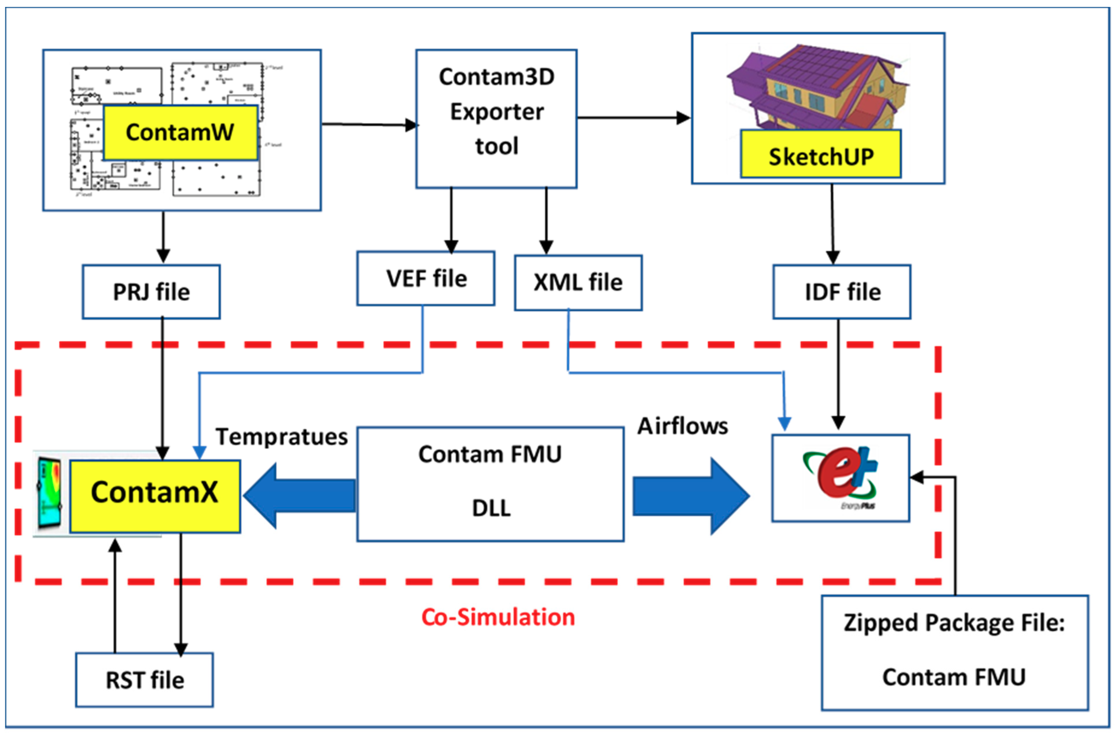
The procedures of the co-simulation approach between EnergyPlus and CONTAM are shown in Figure 1 As shown in this figure, the PRJ file (project file) was designed using the format of CONTAM and the IDF file (input data file) was designed using the format of EnergyPlus. The process initially started with ContamW, which created plan information for each floor of the building as a PRJ file. The information in the PRJ file was entered into ContamX directly, which was the CONTAM simulation engine. On the other hand, the file from the Contam3DExporter tool was converted to an IDF file format. Thus, the initial data could be imported into EnergyPlus. The task of the 3DExporter tool was to convert the PRJ file into two types of VEF file (variable exchange file) and XML file (extensible markup language file) formats. The information in the VEF file and XML file were exchanged during the co-simulation process between ContamX and EnergyPlus according to Figure 1. Finally, the IDF file could be viewed and edited via SketchUp software [39]. This file included geometry, infiltration airflow, inter-zone or mixing airflow, and HVAC system airflow.

During co-simulation, the data transferred from EnergyPlus to CONTAM included the zone temperature, ventilation system airflow, outdoor air fraction, exhaust fan airflow, air temperature, wind speed, biometric pressure, and wind direction information. In addition, the data transferred from ContamX to EnergyPlus included information on the infiltration airflow zone, inter-zone airflow, and the control value of airflow in user-defined contaminant level. Finally, the control variables of the zipped package file, called the Contam FMU (functional mock-up unit), were exchanged and distributed between ContamX and EnergyPlus. ContamX simulated a file with the RST file (restart file) format to synchronize the time of data exchange between the two models within 24 h.

2.3. Governing Equations

The calculations for the heat balance in different zones of the building were performed by EnergyPlus (see Figure 2) in three parts. First, the equations of heat transfer from all interfaces (walls, doors, windows) are described as [29]:

$$E_{conv}={\displaystyle \sum }_{j=1}^N{A}_j{h}_j\left(T_{surf,j}-T_{zone}\right)\left(T_{surf,j}-T_{zone}\right)$$

(5)

where $N$, $A_j$, $h_j$, $T_{surf,j}$, and $T_{zone}$ are the number of surfaces in the room, area of the jth interface, convection coefficient of the jth interface, temperature of the jth interface, temperature of the jth interface, and the zone temperature, respectively. Next, the airflow heat transfer via infiltration–exfiltration and inter-zonal airflow are calculated using [29]:

$$E_{flow,i}= \sum {\dot{M}}_{j\to i}^{air}·C_p^{air}\left(T_{zone,i}-T_{ref}\right)-\sum {\dot{M}}_{i\to j}^{air}·C_p^{air}\left(T_{zone}-T_{ref}\right)$$

(6)

where, ${\dot{M}}_{j\to i}^{air}$, $C_p^{air}$, ${\dot{M}}_{i\to j}^{air}$, $T_{zone,i}$, $T_{ref},$ and $T_{zone}$ are the mass flow rate of air from j to i, specific heat coefficient of air, mass flow rate of air from i to j, temperature of the ith zone, temperature of the reference zone, and temperature of the zone, respectively. Finally, the thermal load of the HVAC system is determined as follows [29]:

$$E_{hvac}= E_{sup}-E_{ret}$$

(7)

$$E_{sup}= {\dot{Q}}_{sup}·{\rho }_{sup}·C_p^{air}·\left(T_{sup,i}-T_{ref}\right)$$

(8)

$$E_{ret}= {\dot{Q}}_{ret}·{\rho }_{ret}·C_p^{air}·\left(T_{zone,i}-T_{ref}\right)$$

(9)

where, $E_{sup}$ and $E_{ret}$ represent the HVAC supply duct heat flow and the HVAC return duct heat flow, respectively (Equation (7)). In Equations (8) and (9), ${\dot{Q}}_{sup}$, ${\dot{Q}}_{ret}$, ${\rho }_{sup}$, ${\rho }_{ret}$, $C_p^{air}$, $T_{sup,i},$ and $T_{zone,i}$ are the supply air duct volumetric flow rate, return air duct volumetric flow rate, supply air duct density, return air duct density, air specific heat at constant pressure, ith supply air duct temperature, and the ith zone air temperature, respectively.

The CONTAM model was used to calculate inter-zone airflow rates, infiltration airflow rates, and HVAC system airflow rates simultaneously for the whole building. The balance of the air mass rate between each node from zone i to zone j in CONTAM is performed using the driving forces as follows [32]:

$${\dot{M}}_{i\to j}^{air} = V_{zone,i}\frac{\partial {\rho }_i^{air}}{\partial t} = {\displaystyle \sum }_j^N\left(s_{i\to j}{K}_g{\left|p_i-p_j\right|}^{n_{i\to j}}\right)+{\dot{M}}_{sup}^{air}-{\dot{M}}_{ret}^{air} = 0$$

(10)

where $V_{zone,i}$, ${\rho }_i^{air}$, $s_{i\to j}$, $K_g$, $p_i$, $p_j$, $n_{i\to j}$, ${\dot{M}}_{sup}^{air},$ and ${\dot{M}}_{ret}^{air}$ are the volume of zone i, density of airflow at zone i, flow direct sign (1 if p_i < p_j and −1 if p_i ≥ p_j), airflow coefficients, pressure field of zone i, pressure field of zone j, flow exponent from zone i to zone j, mass supply airflow rates, and mass return airflow rates, respectively. The mass balance provides the contaminant concentration transfer as follows [32]:

$$\frac{d{m}_i^{\alpha }}{dt} = {\displaystyle \sum }_j{F}_{j\to i}\left(1-{\eta }_j^{\alpha }\right)C_j^{\alpha }+G_i^{\alpha }+m_i{\displaystyle \sum }_{\beta }{K}^{\alpha ,\beta }{C}_i^{\beta }-{\displaystyle \sum }_j{F}_{i\to j}{C}_i^{\alpha }-R_i^{\alpha }{C}_i^{\alpha }$$

(11)

$$R_i^{\alpha } = {\displaystyle \sum }_{\alpha }{R}^{\alpha }{C}_i^{\alpha }$$

(12)

$$C_i^{\alpha } = \frac{m_i^{\alpha }}{m_i}$$

(13)

$$m_i = {\displaystyle \sum }_{\alpha }{m}_i^{\alpha }$$

(14)

The rate of mass gain of contaminant α in control volume i is calculated by Equation (11). Thus, $F_{j\to i}$, $F_{i\to j}$, ${\eta }_j^{\alpha }$, $C_i^{\alpha }$, $C_j^{\alpha }$, $G_i^{\alpha }$, $m_i$, $K^{\alpha ,\beta }$, $C_i^{\beta },$ and $R_i^{\alpha }$ are the rate of air mass flow from control volumes j to i, rate of air mass flow from control volumes i to j, filter efficiency in path j, concentration of contaminants α in control volume i, concentration of contaminants α in control volume j, rate of species generation, mass of air in control volume i, kinetic reaction coefficient in control volume i between contaminants α and β, concentration of contaminant β in control volume i, and the value of the gas constant for the air in control volume i, respectively. In Equation (12), $R^{\alpha }$ is the gas constant of contaminants α and in Equation (13), the concentration of contaminants α in control volume i ($C_i^{\alpha }$) is calculated using the ratio of the mass of the individual contaminants α ($m_i^{\alpha }$) to the mass of air in control volume i ($m_i$). In Equation (14), the mass of air in control volume i ($m_i$) is calculated using the sum of the masses of the individual contaminants α in the control volume i ($m_i^{\alpha }$).

The integrated simulation model can dynamically perform simultaneous heat, air mass, and contaminant mass balances. To solve the governing equations simultaneously, dynamic data is exchanged as control variables by the FMU between EnergyPlus and ContamX. The exchanged parameters from EnergyPlus to ContamX include: zone outdoor temperature, outdoor environment data, ventilation system airflow rates for zone supply and return airflow rates, outdoor airflow fractions of outdoor airflow controllers, exhaust fan airflow rates, and energy recovery fan airflow rates [32]. Furthermore, the exchanged parameters from ContamX to EnergyPlus include: zone infiltration airflow rates, inter-zone airflow rates, and ventilation airflow based on the contaminant level [32]. Finally, by exchanging the data of dynamic control variables, the integrated simulation model can calculate heat, air mass, and contaminant mass transfers, simultaneously, for the whole building.

2.4. Description of the Case Study

In this research study, the simulations of energy consumption (EC) and indoor air quality (IAQ) for a three-story house were performed when it was subjected to two different climatic conditions, namely those in Montreal and Miami.

Table 1. Characterization of the parameters of a three-story house baseline case (reference case).

	Parameter	Range/Type
Geometry	Orientation	0°–180°
	Floor-to-Floor Height	3.6 m
	Floor-to-Ceiling Height	2.7 m
	Window-to-Wall Ratio: S, E, N, W	40%
Envelope	Roof Surfaces	Wood standard (construction), roof, build-up (exterior finish)
	Above Grade Walls	Wood frame, 2 × 6, in on centers (construction); wood/plywood (exterior finish); ¾ in fiberboard sheathing R-2 (exterior insulation)
	Ground Floor	Earth contact (exposure); six-inch concrete (construction); vinyl tile (interior finish)
	Top Floor Ceiling (Below Attic)	Drywall finish (interior finish); metal stud, 24-inch on centers (framing); R-19 batt (batt insulation)
	Ceilings	Plaster finish (interior finish)
	Floors	Vinyl tile (interior finish); six-inch concrete (construction)
Exterior Windows	Double PPG	Starphire/air/clear 6 mm (glass type); aluminum (frame type)
Occupants	A Family of Five People	An adult male, adult female, and three children of ages 5, 11, and 14 years
Age of Construction	22 Years	Renovated 5 years ago

lists the information on geometries, thermal properties, age of construction, and occupancy for the three-story house in the baseline case.

The basement, as a level 1 with a surface area of 24 m² and a volume of 72 m³, had a hot-water heating system, gas furnace, and dryer. At level 2, with an area of 35 m² and a volume of 105 m³, there was a living room with a fireplace, one bathroom, and one closet. Level 3 had a total area of 13 m² and a volume of 50 m³, with two bedrooms and one master bedroom having its own bathroom and closet. The fourth level had an attic with a surface of 13 m² and a volume of 50 m³.

Table 2. Annual standard climate values for 2018 [40,41].

Climate Characteristics
Parameters	Montreal	Miami
Altitude (m)	27	5
Latitude	45°30′N	25°45′N
Longitude	73°25′W	80°23′W
Average Annual Max Temperature (°C)	11	28
Average Annual Temperature (°C)	6	24
Average Min Temperature (°C)	1	21
Average Annual Precipitation (mm)	1017	1420
Annual Number of Wet Days	166	132
Average Annual Sunlight (hours/day)	5 h 05′	8 h 03′
Average Annual Daylight (hours/day)	12 h 00′	12 h 00′
Annual Percentage of Sunny (Cloudy) (daylight hours)	42 (58)	67 (33)
Annual Sun altitude at solar noon on the 21st day	44.8°	64.5°

provides the details of the climate characteristics for Montreal and Miami that were used to simulate a three-story house for different scenarios.

The input data used in the EnergyPlus and CONTAM models included the dimensions, material properties, type of insulation, details of the weather data, type of flow paths, mechanical systems, details on contaminants and filter type, etc. The energy balance was always performed using EnergyPlus. Since the airflow rate can be calculated using CONTAM, this parameter had a very important role in transporting the energy generated by energy sources in HVAC systems. The energy transport by the airflow was transmitted between the inter-zones and the outdoor environment.

The CONTAM project included the geometry, weather data, transient contaminant data, airflow path elements, windows, air-handling systems (AHSs) and filters, duct elements, input controls, sinks and sources of contaminants and species, and other relevant data. Finally, the CONTAM project was created by ContamW in a PRJ file format. In the next step, by running CONTAM3DExport, the PRJ file was converted to an IDF file for EnergyPlus. The IDF file included building geometry, surface materials and constructions, air loops, exhaust fans, and partial external interface objects. The desired HVAC component was added to the IDF file in the IDF Editor to generate or remove energy, heating/cooling coils, internal gains, and thermostats. Also, the IDF file was used to modify the rectangular elements using the Open Studio SketchUp Plug-in tool [39].

The IDF file, along with the ContamFMU.fmu file, were used in the same directory of EnergyPlus. The ContamFMU.fmu file is a zip file and was unzipped during the integrated simulation. This zip file included modelDescription.xml (extensible markup language file), contam.prj (project file), contam.vef (variable exchange file), ContamFMU. .dll (dynamic link library), and contamx3.exe. These files contained parameters and algorithms created by EnergyPlus and was used to exchange the control variables between EnergyPlus and ContamX during the co-simulation process. In the time step setting for the co-simulation, the start and end dates of the contam.prj file in the ContamFMU.fmu file must be set together with the EnergyPlus IDF file. Before starting the co-simulation, the contam.prj and contamx3.exe files of ContamFMU.fmu file were copied to the next directory of EnergyPlus. ContamW then opened the contam.prj file and the co-simulation was set by exchanging control variables between EnergyPlus and ContamX for a single day. At the end of the first day, the CONTAM restart file was generated as a project file used by ContamX during the warm-up period in the co-simulation. At the end of the co-simulation, ContamW could display the output results [32].

In order to show the differences in the results obtained by the single models (EnergyPlus and CONTAM) and those obtained by the present integrated simulation model, a three-story house was simulated when this house was subjected to several climatic conditions in North America. However, this paper presents the results of only two cities: (a) one cold city (Montreal), and (b) one hot city (Miami). The weather data of year 2018 was used in this study. Figure 3 shows the monthly average temperature and relative humidity for Montreal and Miami. The city of Montreal has a humid climate with no dry season. The winters are cold, snowy, icy, and windy, with daily average temperatures from −9 °C to −11 °C [40]. Summers are warm and humid with a daily average temperature between 26 °C and 28 °C [40]. Spring and fall are pleasantly mild but there is a possibility of large changes in temperature in these seasons.

The city of Miami has a tropical monsoon climate. The summer is hot and humid, and the winter is short and warm. In summer, the daily average temperature is between 29 °C to 35 °C and the average relative humidity is 71%. As shown in Figure 3, it also has a winter with a daily average temperature between 20 °C to 24 °C and relative humidity of 79% [41].

3. Results

For the scenarios listed in

Table 3. Status of the proposed scenarios compared to the baseline.

Status		Ventilation Upgrading	Air Tightening	Upgraded Filter
1	Baseline	No	No	No
2	Scenario 1	No	Yes	No
3	Scenario 2	Yes	Yes	Yes

, this section provides the simulation results of: (1) energy consumption (EC) and indoor air quality (IAQ) obtained by the single models for the baseline scenario as a reference, (2) EC and IAQ obtained by the single models for scenario 1, and (3) EC and IAQ obtained by the present integrated simulation model for scenario 2.

The simulated variables in the all scenarios listed in Table 3 include: (a) air exchange rates, (b) indoor particle concentrations, (c) indoor CO₂ concentrations, and (d) the electrical and gas energy consumptions. In scenario 1, the single models of EnergyPlus and CONTAM were used independently to simulate these variables. The variables of scenario 2, however, were simulated by the present integrated simulation model. In order to better evaluate the models’ accuracy, the variables of scenario 2 were also simulated by the single models. In this case, we can easily show the differences between the results obtained by the single models and those obtained by the present integrated simulation model.

3.1. The Baseline Case

In the baseline, the air change rates and concentrations of indoor contaminants for CO₂ and particles were simulated under the different climatic conditions of Montreal and Miami. The three-story house for a population of five persons was defined as having an air handling system (AHS) of 0.40 m³/s and a MERV (minimum efficiency reporting value) 4 filter for the baseline. PM₅ particles in the range of 5.0 µm to 10 µm were considered in this research study. Concentration rate values were considered for indoor particles sources based on the measurements by Elbayoumi et al. [42]. Given that one of the sources of indoor CO₂ generation is the occupants, its concentration values were assumed to be 24.4 mg/s for sleeping status and 40 mg/s for awake status according to the ASHRAE (American society of heating, refrigerating and air-conditioning engineers) standard [43]. Another source of CO₂ is the outdoor air with a concentration of 348.57 ppm (630 mg/m³) [44].

For Montreal, the outdoor particle concentrations used were based on the measurements by Smargiassi et al. [45]. Also, the outdoor particle concentrations used for Miami were based on the measurements by Cao et al. [46].

3.2. Results of Scenarios 1 and 2

For scenario 1, only the airtightness of the building enclosure was improved by 45% of the baseline scenario. Scenario 2, however, included a combination of enclosure air tightening, ventilation upgrading to exhaust fans, and filter upgrading to MERV (minimum efficiency reporting value) 12.

For Montreal and Miami, the simulation results obtained using CONTAM, EnergyPlus, and the present integrated simulation models for both scenarios 1 and 2. The minimum, average, and maximum values of air change rates, indoor particle concentrations PM₅, indoor CO₂ concentrations, and electrical and gas energy consumptions are shown in Figure 4, Figure 5, Figure 6, Figure 7 and Figure 8.

For different climatic conditions,

Table 4. Comparisons of energy consumption (EC) and indoor air quality (IAQ) measures for the baseline and scenarios 1 and 2 based on a percentage of average changes.

	Percentage Ratio of Average Decrease (↓) or Increase (↑) Annual Values of Each Scenario Relative to Baseline Measures (%)
Measures	Air Change Rates		Indoor Particles Concentrations (PM5)		Indoor CO2 Concentrations		Electrical Energy Consumptions		Gas Energy Consumptions
Cities	Montreal	Miami	Montreal	Miami	Montreal	Miami	Montreal	Miami	Montreal	Miami
Scenario 1	70% ↓	65% ↓	16.7% ↑	2.4% ↑	44.6% ↑	43.6% ↑	14.2% ↓	28.4% ↓	44.3% ↓	35.2% ↓
Scenario 2	26% ↓	20.9% ↓	21.8% ↓	4.7% ↓	3.7% ↓	7.8% ↓	2.6% ↓	15.2% ↓	34% ↓	22.5% ↓

compares the percentage of the average decrease (↓) or average increase (↑) in the annual values of each scenario in relation with the baseline measures for the air change rates, indoor particle concentrations PM₅, indoor CO₂ concentrations, and gas and electrical energy consumptions.

Figure 4, Figure 5, Figure 6, Figure 7 and Figure 8 show the simulation results (air change rates, indoor particle concentrations PM₅, indoor CO₂ concentrations) obtained by CONTAM and the results obtained by EnergyPlus (gas and electrical energy consumptions). These results were obtained for two different climates (Montreal and Miami).

4. Discussion

Given the improved energy consumption due to the envelope airtightness in scenario 1, this condition negatively affected both the indoor air quality (IAQ) and air exchange rates. The air change rate values in scenario 1 are shown in Figure 4a,b for each of the two different cities of Montreal and Miami, respectively. Based on ASHRAE 62.2 [48], the air change rates should not be below the rate of 0.35 h⁻¹. In Montreal, the average air change rates in the fall, winter, summer, and spring were calculated to be 0.21 h⁻¹, 0.33 h⁻¹, 0.2 h⁻¹, and 0.33 h⁻¹, respectively, which were below the ASHRAE standard value. Additionally, in Miami (see Figure 4b), the average air change rates in scenario 1 were also below the ASHRAE 62.2 standard for all seasons of fall, winter, spring, and summer (0.11 h⁻¹, 0.15 h⁻¹, 0.16 h⁻¹, and 0.13 h⁻¹, respectively).

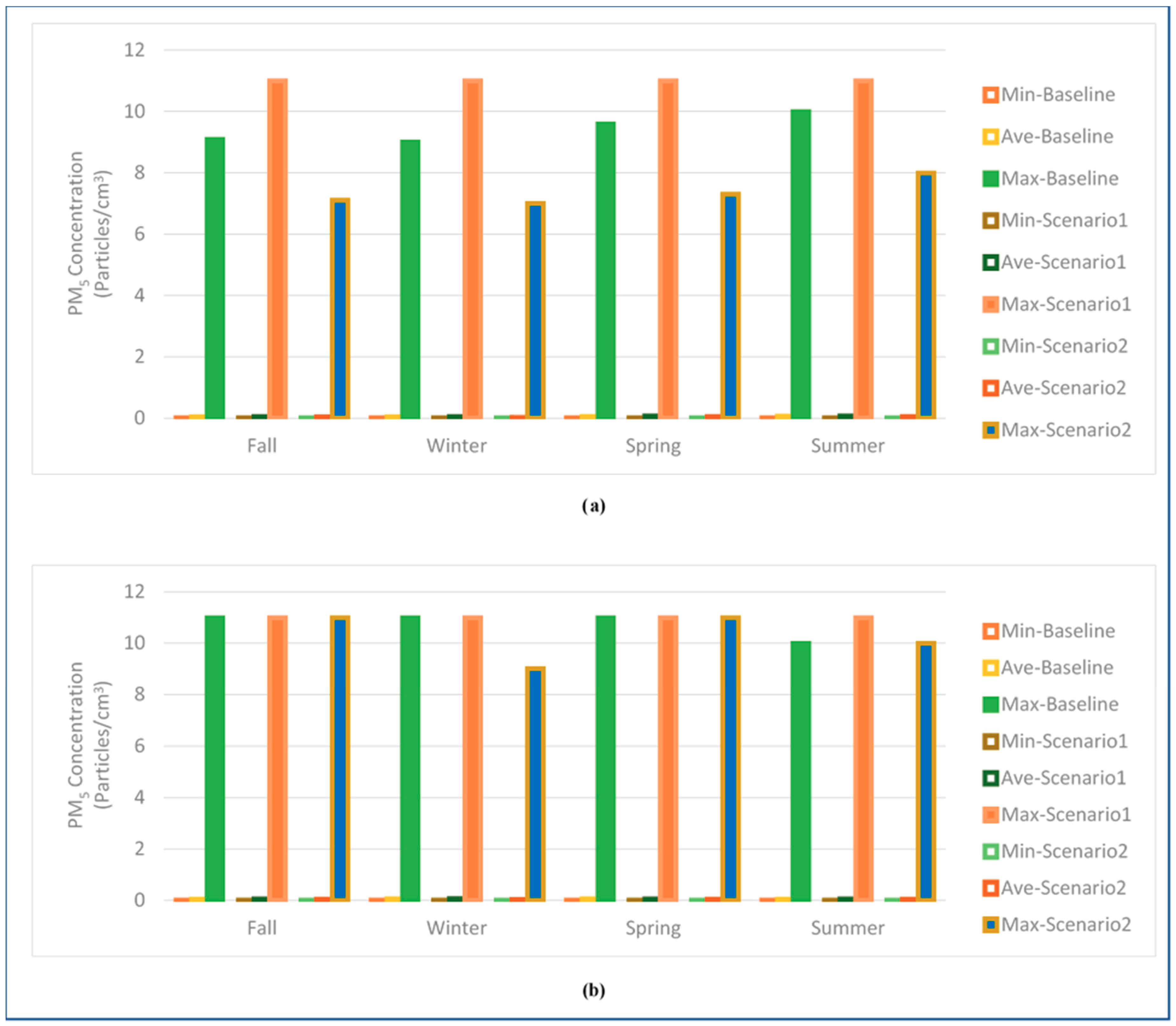
The obtained values for the concentrations of indoor contaminants in scenario 1 are shown in Figure 5 and Figure 6 for Montreal and Miami. In scenario 1, the average concentration of indoor particles (PM₅) in the two cities were the same value of 3.68 particles/cm³ (Figure 5a,b). Furthermore, the average indoor CO₂ concentrations for the cities of Montreal and Miami were calculated to be 1280 mg/m³ and 1554.17 mg/m³, respectively (Figure 6a,b). Therefore, it can be concluded that scenario 1 in Miami was a worse case than Montreal in terms of the indoor CO₂ concentration.

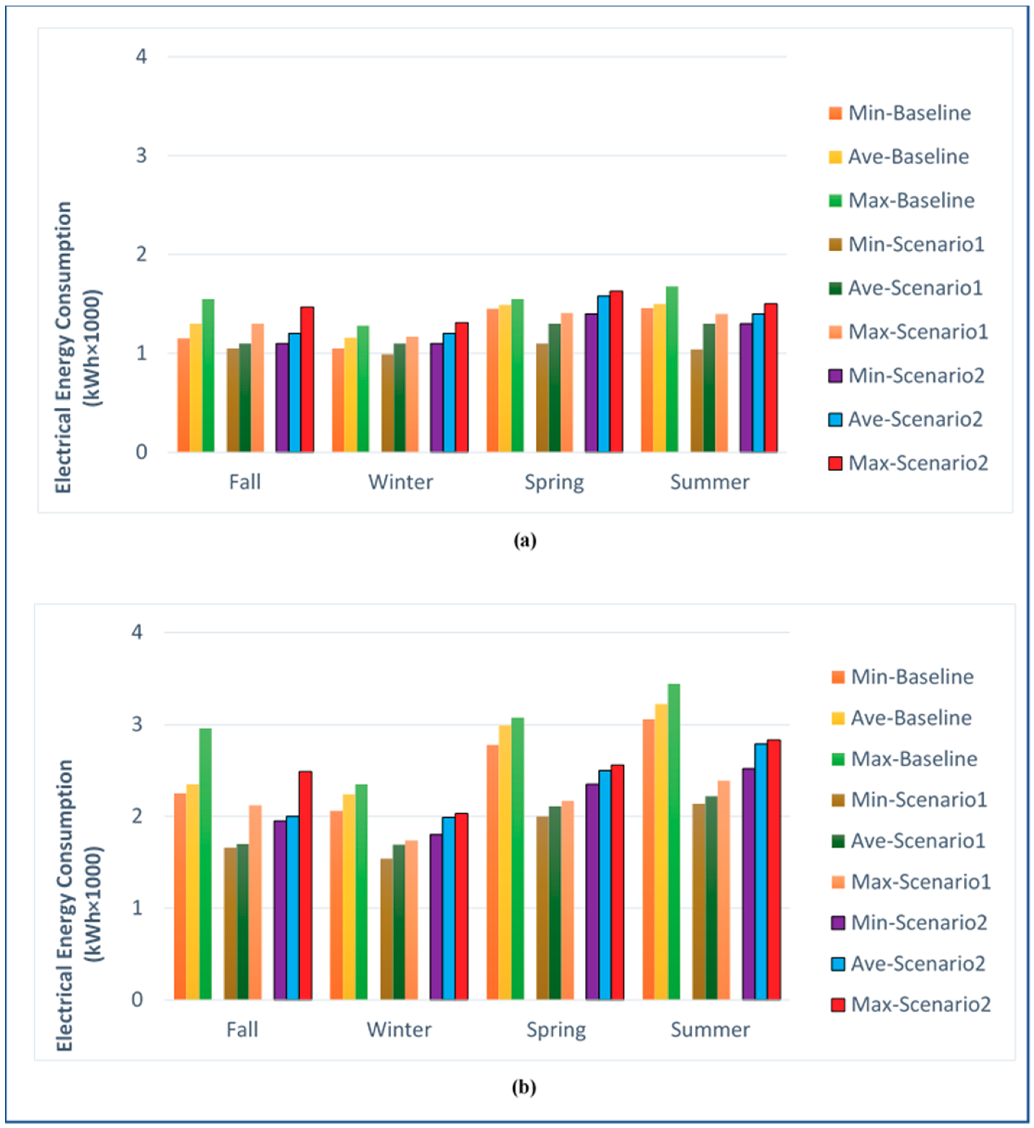
Regarding the energy performance, the envelope airtightness in scenario 1 resulted in reducing the energy consumption (EC) where the highest annual average decrease ratio of the air change rates in relation with the baseline scenario for the city of Montreal was 70%. This decrease in this ratio resulted in air change rates of less than 0.35 h⁻¹, which is not recommended by the ASHRAE 62.2 standard [48].

To improve EC in scenario 2, the exterior envelope was more airtight, i.e., 42% higher than the baseline. Also, to improve the IAQ in scenario 2, an exhaust fan with a capacity of 26 L/s was changed to continuous ventilation. A highly efficient particle air filter (MERV 12) was used to further reduce the indoor particle concentration. The improvements in the EC and IAQ obtained with the present integrated simulation model in scenario 2 are provided in Table 4.

In scenario 2, the results for the case of envelope airtightness, and exhaust fan installations were obtained using the integrated simulation model where the filter was upgraded from a MERV 4 to a MERV 12 AHS. Therefore, the possibility of a simultaneous controlled improvement of EC and IAQ could be investigated. Scenario 2 could therefore have the greatest impact on both the reduction in the electrical and gas consumption and the reduction in the indoor contaminant concentrations. By comparing the EC parameters, it was observed that scenario 2 had the highest annual average decrease ratio of electrical and gas energy consumptions compared to the baseline scenario for Miami and Montreal cities by 15.2% and 34%, respectively.

In Miami, the improvement in EC was due to the controlled envelope airtightness and exhaust fan ventilation status in scenario 2, which had the greatest effect for hot cities, such as Miami in reducing the consumption of electrical energy to the space cooling of the whole building for hot days compared to the other scenarios. On the other hand, the same improvement in scenario 2 in Montreal has the greatest impact on reducing the gas energy consumptions due to a lower need for gas fuel for space heating of the whole building on very cold days. In terms of decreasing the indoor contaminant concentrations, the integrated simulation model calculated the greatest impact of scenario 2 on the annual average decrease ratio of indoor particulate (PM₅) concentrations and indoor CO₂ concentrations to the baseline scenario to be 21.8% for Montreal and 7.8% for Miami.

According to Table 4, the difference of electricity consumption in scenario 1 with the baseline obtained by EnergyPlus for Montreal and Miami were calculated to be −14.2% and −28.4%, respectively. The difference in electricity consumptions between scenario 2 and the baseline were obtained from the present integrated simulation model for Montreal and Miami to be −2.6% and −15.2%, respectively. Additionally, the difference in gas energy consumptions obtained by EnergyPlus relative the baseline for scenario 1 for Montreal and Miami were calculated to be −44.3% and −35.2%, respectively. If the integrated simulation model was used to calculate the difference in gas energy between scenario 2 and the baseline, this difference was −34% and −22.5% for the cities of Montreal and Miami, respectively (see Table 4).

Table 4 shows that the differences between the air change rates obtained by CONTAM for scenario 1 in Montreal and Miami were calculated to be −70% and −65%, respectively. However, the difference between the results of the air change rates obtained by the present integrated simulation model for scenario 2 in Montreal and Miami was calculated to be −26% and −20.9%, respectively. Note that the EC and IAQ results of scenario 1 were only obtained with the single CONTAM model, EnergyPlus model, and the result of scenario 2 obtained by the present integrated simulation model. Table 4 shows the differences between the results of the two scenarios and the baseline scenario.

The ultimate goal of this study was to examine the differences in the results obtained by the integrated simulation model and single models. To this end, scenario 2 was chosen as a reference and

Table 5. Simulated average annual results of the total energy consumptions and the air change rates using single models of EnergyPlus and CONTAM versus integrated simulation model for scenario 2.

Scenario 2 Results	Montreal		Miami
Average Annual Total Energy Consumptions (GJ)	EnergyPlus	Integrated Simulation Model	EnergyPlus	Integrated Simulation Model
	25.536	21.184	19.283	17.296
Average Annual Air Change Rates (h−1)	CONTAM	Integrated Simulation Model	CONTAM	Integrated Simulation Model
	0.597	0.538	0.445	0.318

shows the average annual total energy consumptions and air change rates. As shown in this table, the average annual total energy consumptions for scenario 2, simulated using EnergyPlus, were 25.536 GJ and 19.283 GJ, and the corresponding values obtained by the integrated simulation model were 21.184 GJ and 17.296 GJ for Montreal and Miami, respectively. Also, Figure 9 shows that the differences between the average annual total energy consumptions simulated by EnergyPlus versus the integrated simulation model were 4.352 GJ and 1.987 GJ, respectively, for Montreal and Miami.

The simulation results of the average annual air change rates by CONTAM for scenario 2 were 0.597 h⁻¹ and 0.538 h⁻¹ for Montreal and Miami, respectively (see Table 5). These simulated IAQ measures for scenario 2 using the integrated simulation model were 0.445 h⁻¹ and 0.318 h⁻¹ for Montreal and Miami, respectively. Additionally, the differences between the average annual air change rates simulated using the CONTAM versus that simulated using the present integrated simulation model were 0.059 h⁻¹ and 0.127 h⁻¹ for Montreal and Miami, respectively (Figure 10).

The differences in the energy consumptions and the air change rates shown in Table 5 and Figure 9 and Figure 10 were significant. The energy consumption difference was higher in the cold climate in Montreal because a well-insulated house consumes less energy in a warm climate. In Miami, this difference was about 10 percent.

5. Conclusions

In this research study, an integrated simulation model was developed using a co-simulation method that can be used to simultaneously predict the energy consumption (EC) and indoor air quality (IAQ) performance for buildings subjected to different climatic conditions. The CONTAM model and the EnergyPlus model were integrated to develop this model. Because of the interactive/coupling of EC and IAQ, the predicted results with the present integrated simulation model were more realistic than those obtained with the single models. The present integrated simulation model addressed the computational limitations of the EnergyPlus and CONTAM single models by dynamically exchanging the simulated real-time temperatures and the simulated airflow rates. In order to show the differences in the results for the EC and IAQ performance obtained using the present integrated simulation model and those obtained using a single model, two scenarios were conducted for a three-story house when this house was subjected to the different climatic conditions of two cities in North America (Montreal and Miami).

The results of the single models and the integrated simulation model for the energy performance were compared in Figure 9 and Table 5. Additionally, the results of the single models and the integrated simulation model for the IAQ performance were compared in Figure 10 and Table 5. These comparisons showed that due to the opportunity to exchange the correct temperature and airflow rate variables simultaneously in the present integrated simulation model, the difference between the EC-IAQ results with the baseline indicates the improvement in assessing the performance of the buildings. Finally, considering the energy consumption and indoor air quality results obtained from the single models (EnergyPlus and CONTAM) and comparing them with those obtained from the present integrated simulation model for Montreal and Miami, it was found that the results of scenario 2 found using co-simulation were better than other scenarios for improving EC and IAQ together.

This research study, called “Part 1,” generated some energy savings caused by the specific construction measures but we do not dwell on their interpretation as the objective of the paper was to demonstrate the need for changing the paradigm of thinking. By moving from the individual (i.e., uncoupled) models to an integrated system, we are basically reducing the gap between models and practice. It is important to point out that the limitation of this research study was that the moisture transport in the building envelope was not accounted for. The next step in our research, which is in progress, is to conduct another study, called “Part 2,” which introduces liquid and vapor forms of water movements in building envelopes. In Part 2, a heat, air, and moisture (HAM) transport model is currently being coupled with the present integrated simulation model in order to simultaneously assess: (a) the energy performance, (b) indoor air quality performance, and (c) the risk of condensation and mold growth inside the building envelope. The obtained results for the building envelope of different cladding systems, subjected to different climatic conditions of North America, will be published at a later date.