Abstract
To better track the planned output (forecast output), energy storage systems (ESS) are used by wind farms to compensate the forecast error of wind power and reduce the uncertainty of wind power output. When the error compensation degree is the same, the compensation interval is not unique, different compensation intervals need different ESS sizing. This paper focused on finding the optimal compensation interval not only satisfied the error compensation degree but also obtained the max profit of the wind farm. First, a mathematical model was proposed as well as a corresponding optimization method aiming at maximizing the profit of the wind farm. Second, the effect of the influencing factors (compensation degree, electricity price, ESS cost, and wind penalty cost) on the optimal result was fully analyzed and deeply discussed. Through the analysis, the complex relationship between the factors and the optimal results was found. Finally, the comparison between the proposed and traditional method was given, and the simulation results showed that the proposed method can provide a powerful decision-making basis for ESS planning in current and future market.
1. Introduction
Wind power as a kind of high-quality renewable energy, has developed rapidly in the recent years. With the increasing penetration of wind power, it generates a large quantity of clean electricity for the power grid. At the same time, the uncertainty of wind power output also poses a huge challenge to the safety and reliable operation of the power grid [1].
Energy storage systems (ESS) provide fast response capacity for the power system. It is characterized as dynamic energy absorption and timely release. With ESS, it is possible to make the time transfer of power and energy, and achieve the balance of power and energy in the power system under various operating conditions. A better configuration of the ESS in the power system can improve the capacity of the grid to absorb the wind power, enhance the dispatchability of wind power, and ensure the safe operation of the power grid [2].
Due to the relatively high cost of the ESS, how to optimize the ESS sizing according to different needs and purposes has become a hot topic. Many references have discussed the optimization of the ESS sizing. At present, the research on ESS sizing planning mainly includes smoothing the short-term fluctuation of wind power output [3,4], dealing with the peak shaving problem of power systems with wind power [5,6], and compensating the forecast error of wind power output, and so on.
The forecast error of wind power is inevitable because of the characteristics of wind power generation. The ESS is installed at the outlet of the wind farm to compensate the forecast error of wind power and ensure that the wind farm can output the power reliably according to the pre-declared plan. In real-time dispatching, the ESS can store or release energy to balance the corresponding power error when the real-time power value of a wind farm is different from the planned output. In terms of compensating wind power forecast error, there are many references discussing this top from different aspects [7,8].
The authors of [9] optimized the capacity of energy storage devices by controlling the wind power forecast error within a certain range to minimize the cost of energy storage equipment. In [10] the authors optimized the capacity of energy storage devices with the objective of minimizing wind power prediction errors. By quantifying the functional relationship between energy storage capacity and unserved energy, the minimum energy storage capacity corresponding to different unserved energy is analyzed. The authors of [11] synthetically considered the energy efficiency, environmental benefit and one investment of wind power and ESS, constructed the corresponding economic evaluation model, and evaluated the feasibility of using ESS to improve the wind power acceptance scale in different dispatching risk scenarios. The authors of [12] reduced the impacts of wind power forecast errors while prolonging the lifetime of ESS. In [13] the authors used a simple autoregressive model to capture the stochastic behavior of day-ahead forecast errors, in particular the autocorrelation structure of these errors, and parametrically assessed the storage performance using a MAD criterion. In [14], a mixed distribution was proposed based on Laplace and normal distribution to model forecast errors, then a probabilistic method was proposed to determine the optimal size of ESS for wind farms in electricity markets.
Based on the previous works, in this study, we proposed optimal planning of the ESS sizing in several new ways.
First, in order to compensate the wind power error to some extent, the concept of error compensation degree should be considered. Most published reports did not discuss that at the same error compensation degree, the corresponding error compensation interval is not unique and then the needed ESS sizing is also different. How to find the optimal error compensation interval among these intervals becomes an important problem to be solved. In this paper, we established a mathematical model and proposed an optimization method to find the optimal compensation interval which not only can satisfy the compensation degree but also can maximize the profit of the wind farm.
Second, based on the forward-looking consideration, in the future, some factors such as electricity price, ESS cost, and wind penalty cost may change. If these factors change, the optimization result will be different. However, previous studies only discussed their effects from limited aspects, such as under a certain compensation degree or in a certain cost condition. No complete analysis was available. An incomplete analysis may mislead the decision maker’s judgments. In this paper, a thorough analysis about the effects of these factors on the ESS optimization result was carried out. The sensitivity of each factor on the optimal result was analyzed in detail, and the valuable investment range was discussed.
Finally, a simulation of the above methods was performed. Results showed that compared with the traditional method, the comprehensive work in this paper obtained an optimal ESS sizing and the max profit under the same compensation degree. This work provided a powerful decision-making base for ESS planning in current and future markets.
2. ESS Compensation for Wind Power Forecast Error
The purpose of ESS in this paper is to compensate the forecast error of wind power and enable the wind farm to track the planned output. According to the planned output curve, the charging and discharging process of the ESS is controlled to make the actual output power of wind farm as close as possible to the planned output [15,16]. Here, the day-ahead forecast output of a wind farm is regarded as the planned output.
The sizing of ESS is based on the wind power forecast error. The ESS compensates the difference between the actual wind power and the planned wind power (i.e., the forecast error e) in real time, so that the wind farm can act as a power source with steady output and complete the planned generation as the conventional power source.
In this case, the size of ESS is related to the accuracy of wind power forecast [17]. The smaller the error, the smaller the ESS size required.
2.1. Analysis of Power Forecast Error
Configuring an appropriate ESS in the wind farm could make the regulation and control of the power grid more flexible. The ESS can decrease the uncertainty caused by the wind power forecast error to meet the goal of tracking the planned output.
The ESS sizing optimization method proposed in this paper was based on wind power forecast error. There is a certain error between the forecast output and the actual output of wind farm [18,19]. According to the wind farm forecast error, the rated power and rated capacity of the ESS are determined [20,21].
As shown in Figure 1, the green curve represents the actual wind power (Pactual), the blue curve represents the forecast power (Pforecast), and the error of wind power forecast (e) is shown in Figure 2, the red curve.
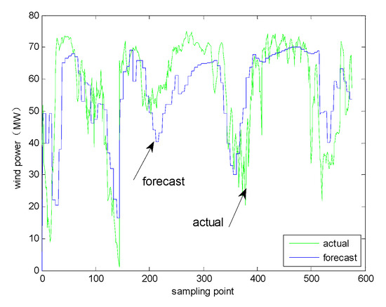
Figure 1.
Wind power forecast output and actual output.
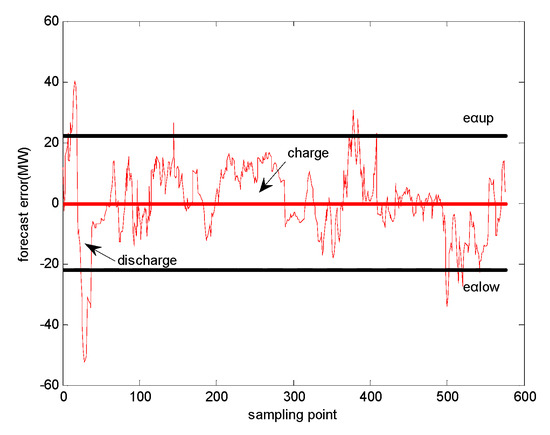
Figure 2.
Wind power forecast error and the confidence interval.
By analyzing the historical forecast error data of wind power, the distribution law of the forecast error can be found, and then the confidence intervals of errors under different confidence degrees can be obtained. The upper and lower bound of the confidence intervals are written as (eαlow eαup). Here, we suppose the error obeys the normal distribution which is used commonly [22,23,24,25,26]. The method in this paper is applicable for both normal distribution and other distributions. If the confidence degree is α%, as shown in Figure 3, the meaning of confidence interval (eαlow eαup) is that the α% probability of forecast error falls into the interval (eαlow eαup).
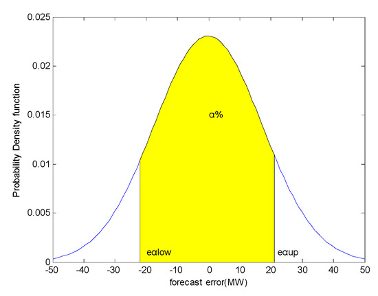
Figure 3.
Probability density function.
2.2. Determination of the ESS Rated Power
In order to track the planned output of the wind farm, the ESS is used to compensate the forecast error of the wind power, so that the actual output of wind farm follows the planned output (forecast output). When error > 0, that is, when the actual output of wind power is greater than the forecast output, the ESS charges and the wind farm will be free from the penalty of wind curtailment; when error < 0, that is, when the actual output of wind farm is less than the forecast output, the ESS discharges, which avoids the penalty of power shortage caused by the lack of electricity in the wind farm. By installing appropriate energy storage devices at the outlet of the wind farm, the output of the wind farm is as close to the planned output (forecast output) as possible [17].
The probability of large wind power forecast error is small if considered just from the point of probability. In order to compensate for the large error of small probability, it is necessary to install a larger rated power ESS. However, this will lead to a significant increase in the cost of ESS. To better assist in choosing of an optimal capacity of ESS, the concept of error compensation degree is considered.
The error compensation degree is that the ESS compensates wind power forecast error.
When the ESS compensates all forecast errors, i.e., the error compensation degree is 100%, the rated power of the ESS is the maximum absolute value of the forecast error.
When the ESS compensates forecast error, we call the error compensation degree . At this time, the error compensation interval is (), is the lower bound of the compensation interval, is the upper bound of the compensation interval.
The required ESS rated power is the maximum absolute value of the upper and lower bounds of the confidence interval, i.e.,
Figure 2 also shows the charging and discharging power of the ESS with time when the compensation degree is . Here the compensation degree is the confidence degree of error.
2.3. Determination of the ESS Rated Capacity
Due to the different dispatching and operation plans of power grid, the optimal ESS rated capacity is different. In this paper, the time window is taken as one day to configure the ESS rated capacity [27].
By accumulating the charge and discharge of ESS at each sampling time, the energy fluctuation of ESS relative to the initial state at different sampling time can be obtained as Equation (4).
where, is the energy fluctuation of ESS at the nth sampling time relative to the initial state, i.e., the sum of accumulative charge and discharge of the ESS in the first n sampling periods. The unit is MWh;
PESS [i] is the actual charging and discharging power of the ESS;
are the upper and lower bounds of the compensation interval when the compensation degree is ;
is the sampling period. The sampling period in this paper is 10 min, i.e., 1/6 hour, the unit is hours;
n is the number of samples in a scheduling cycle. If the time window is one day, then n = 1, 2, …, 144;
i is the nth sampling point.
According to the energy fluctuation in the whole sample data period, the difference between the maximum and minimum energy fluctuation can be calculated [5]. Considering the limitation of the state of charge (SOC), the capacity required for the ESS can be obtained, that is, the rated capacity of the ESS.
where,
is the rated capacity of the ESS, see Equation (6);
are the maximum and minimum energy changes relative to the initial state in the whole sample data cycle, respectively;
Sup and Slow are upper and lower limit constraints of the state of charge (SOC) of the ESS, respectively. In practice, in order to avoid over-charging and over-discharging in actual operation of the ESS, the values should be appropriately taken in [0, 1]. In this paper, the values are 0.9 and 0.1.
When the compensation degree is 100%, that is, the ESS can completely compensate the wind power forecast error, the in Equation (4) is the forecast error e itself of each sampling time.
When the compensation degree is , that is, when the ESS compensates error, is as shown in Equation (5).
3. Optimization of the ESS Sizing with Economic Objective
The purpose of optimization of the ESS is to minimize the rated power and rated capacity of the ESS so as to maximize the profit of the system on the premise of satisfying the compensation degree requirements.
In order to optimize of the ESS sizing under a certain compensation degree, the compensation interval of forecast error under this compensation degree should be obtained first. It is noted that under the same compensation degree, the error compensation interval is not unique. We need to find the optimal interval, and then obtain the optimal ESS sizing to maximize the profit of the wind farm.
3.1. Objective Function
Considering the economic index of wind energy storage system [11,20], in this paper, the objective function is to maximize the profit of the wind farm after installing the ESS [9,11].
where,
f is the objective function, the profit of the wind farm after installing ESS;
is the income of extra generated electricity after installing ESS in the wind farm;
is the cost of ESS [21];
is the cost of the wind curtailment penalty and wind shortage penalty [26];
where,
c is the electricity price;
Esell is the amount of extra generated electricity after installing ESS in the wind farm, measured in MWh; in fact, the extra generated electricity of the wind farm is the amount of electricity charged and discharged by the ESS.
is the charge and discharge power of the ESS, as shown in Equation (5).
where,
is the unit power cost of the ESS, measured in $/MW/per day [27];
is the rated power of the ESS, measured in MW, see Equation (3);
is the total power cost of the ESS;
is the unit capacity cost of the ESS, measured in $/MWh/per day;
is the rated capacity of the ESS, measured in MWh, see Equation (6);
is the total capacity cost of the ESS;
where,
is the unit wind curtailment penalty, measured in $/MWh;
Ecurtail is the amount of wind curtailment, measured in MWh;
is the total cost of wind curtailment;
is the unit wind shortage penalty, measured in $/MWh;
the amount of wind shortage, measured in MWh;
is the total cost of wind shortage;
where,
is the error of each sampling time, is the sampling period, in this paper is 10 min;
is the upper bound of the compensation interval;
is the lower bound of the compensation interval.
3.2. Constraint Conditions
Constraints on rated power of ESS:
Constraints on upper and lower bounds of error confidence intervals:
is the probability distribution function of errors.
3.3. Solving Steps
The above optimization problem can be expressed as follows:
where,
f is the profit of the wind farm after installing ESS, see Equation (7);
g is the inequality constraint, see Equation (14);
h is the equality constraint, see Equation (15);
The flow chart of solving this optimization problem is shown in Figure 4.
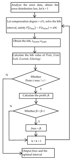
Figure 4.
Flow chart of solving the optimization problem.
4. The Analysis of Influencing Factors on the Optimal Result
Some influencing factors, such as error compensation degree, electricity price, ESS cost, wind curtailment penalty cost, and wind shortage penalty cost, have an impact on the optimal results (the optimal compensation interval, the optimal ESS sizing, and the max profit) [20]. That is to say, in the optimization model, the change of the coefficients (C, CP, CE, C1, C2) in the objective function, see Equation (7), will influence the optimal result. A detailed and complete analysis of these factors is important to improve ESS planning by decision makers. The effect of these factors on the optimal results is analyzed in this section.
4.1. The Effect of Error Compensation Degree
Different error compensation degrees will lead to different max profits and different optimal ESS sizing. In some cost conditions, with the increase of the compensation degree, the max profit may increase, while in other cost conditions, the greater the compensation degree, the less profit. An example of the detailed analysis of the relationship between the error compensation degree and the optimal results was presented in the case study in the following section.
4.2. The Effect of Electricity Price
The major source of the profit of the electricity power system comes from the sales income, which is determined by the electricity price and electricity sales amount. The interaction of pricing mode, market mechanism, and profit model is still largely under investigation. What is clear is that if the electricity price rises to a reasonable value, to increase the total profit, the system will configure a larger ESS capacity to increase energy storage and sales, and meanwhile to reduce the power shortage. On the other hand, ESS has no investment value if the electricity price is below a certain lower limit. Thus, there is a reasonable “price range” for the wind power storage system. The reasonable price range is discussed through the simulation in detail in the following section.
4.3. The Effect of the ESS Cost
Currently the ESS cost is still high. However, with the development of energy storage technology and the related supporting policies, the ESS cost is expected to be reduced in the future. This will eventually lead to enlarged energy storage sizing in the electricity power system. The effect of different ESS unit costs on the ESS optimal result was analyzed in detail in the simulation section.
4.4. The Effect of the Penalty Cost
Due to the special nature, the wind power generation cannot reach the stability level as the conventional power source. If the planned curve is used to evaluate it, there will inevitably be wind curtailed [21] and wind shortage. If the wind farm curtails power, the electricity generated by the wind farm will be decreased. The wind farm can avoid the penalty of the curtailed wind if the ESS compensates these curtailments. Equivalently, this also means the wind farm generates extra electricity (we call it the extra electricity). If there is a shortage of electricity, the wind farm will have to buy electricity from the grid to maintain its planned output. The wind curtailment penalty unit cost and wind shortage penalty unit cost reflect the stringent requirement of power generation controllability for wind farms. The higher the penalty unit cost is, the higher the requirement for the controllability.
5. Case Studies
Field data of a wind farm in Ohio from 1 January to 31 December 2013 was analyzed in this paper. The sampling interval was 10 min, the time window was one day, and the maximum output of the wind farm was 150 MW. Lithium batteries were used for the ESS. The lifetime of the ESS was 20 years. The main purpose of the ESS was to keep the output of the wind farm following the planned output well.
5.1. Analysis of Wind Power Forecast Error
Based on the historical forecast error of wind farm, the distribution law of the error was analyzed. As we did not focus on the error distribution in this paper, the assumption was that the error obeys the normal distribution which is most widely accepted by most researchers [18,22,23,24,25,26]. This method was also compatible for other distributions. The actual error data and the probability density function is shown in Figure 5. The mean value and the standard deviation were calculated to be −0.146 and 17.299, respectively.
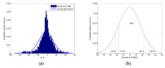
Figure 5.
Wind power forecast error: (a) the actual error data and the normal distribution; (b) different confidence intervals when the confidence degree is 80%.
A confidence degree of 80% was used as an example in this analysis. If 80% of the forecast errors were compensated, or when the compensation degree was 80%, the ESS rated power should be the maximum of the absolute value of the upper and lower bounds. The ESS rated capacity can be calculated by Equation (6).
It was noticed that, when the compensation degree was the same, the compensation interval was not unique. As shown in Figure 5b, with the same 80% compensation degree, compensation intervals were different, and so were the ESS rated power and ESS rated capacity.
If 80% of the forecast errors were compensated, there were 20% of the errors remaining not compensated. Therefore, the wind farm would have a certain amount of curtailed wind and shortage wind, as shown in Figure 5.
5.2. The ESS Sizing Optimization Considering Economic Objective
Through calculation (see Section 3), the range of ESS rated power was from 22.31 to 44.41 MW, and the range of ESS rated capacity was from 88.57 to 151.81 MWh. To maximize the profit of the wind farm, the problems to be solved in this section were how to find the optimal compensation interval, then the optimal ESS rated power and rated capacity.
The objective function is shown in Equation (7), and the constraints are shown in Equations (14) and (15). Lithium batteries were selected for the ESS, and the unit costs were unit power cost, 857,000 $/MW/per day; unit capacity cost, 357,000 $/MWh/per day; electricity price, 85.7 $/MWh; wind power curtailment penalty, 85.7 $/MWh; wind power shortage penalty, 85.7 $/MWh [5,11,16,26].
Through optimization calculation, the optimal result was obtained. Taking 80% compensation degree as example, the optimal compensation interval was [−22.02, 22.31]. Thus, the optimal configuration of the ESS was 22.31 MW for the rated power and 108.94 MWh for the rated capacity. At this time, the max profit for one day was $9089.05. The extra generated electricity, curtailed wind, and wind shortage were 252.03, 39.47, and 13.76 MWh, respectively (Table 1).

Table 1.
Optimal result when the error compensation degree is 80%.
The objective function (wind farm profit) varied with the ESS capacity. When the ESS capacity was 108.94 MWh, the profit reached the maximum, as shown in Figure 6a.
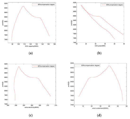
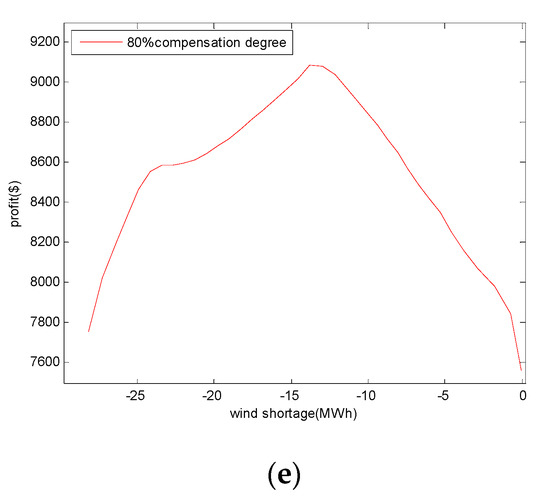
Figure 6.
The relationships between the profit and some factors: (a) profit and the energy storage systems (ESS) capacity; (b) profit and the ESS power; (c) profit and the extra electricity; (d) profit and the wind curtailment; (e) profit and the wind shortage.
The relationships between the profit and other factors are shown in Figure 6b–e.
5.3. The Comparison of the Optimization Method in This Paper with the Traditional Method
When solving the confidence interval, the traditional method is the symmetric point method. However, this method did not consider that the corresponding confidence interval is not unique when the confidence degree is the same. If the traditional method (symmetric point method) was used to find the compensation interval, the results were different. The traditional method (symmetric point method) can obtain the shortest interval when the distribution is normal distribution. However, the shortest interval does not necessarily mean the optimal interval.
In order to compare the proposed method with the traditional method (symmetric point method), the compensation interval, the interval length, the profit (one day), the ESS rated power (Prate), and ESS rated capacity (Erate) were calculated, and the results are shown in Table 2.
Table 2.
Result comparison between the optimization method in this paper and the traditional method.
From Table 2, we can find that at every compensation degree, the traditional method (symmetric point method) always obtained the shortest interval, the optimization method proposed in this paper always obtained the maximum profit. The shortest interval is not necessarily the optimal interval. It was also noticed that at 85% and 80% compensation degrees, the traditional method (symmetric point method) also obtained the max profit as the proposed method, meaning that at these two compensation degrees, the shortest interval was also the optimal interval. However, at other compensation degrees, the results were different, which means the shortest interval was not necessarily the optimal interval.
To sum up, the method in this paper can always obtain the max profit under the same compensation degree. Through the proposed method, the optimal ESS rated power (Prate) and the optimal ESS rated capacity (Erate) also can be obtained.
5.4. The Result Analysis
An example of one day, Figure 7 shows the actual power and forecast power of the wind farm. Figure 8 shows the forecast error and the optimal compensation interval under 80% compensation degree. Figure 9 demonstrates the ESS charging and discharging of the optimal configuration. Figure 10 shows the actual output of the wind farm after compensating the forecast error by the ESS.
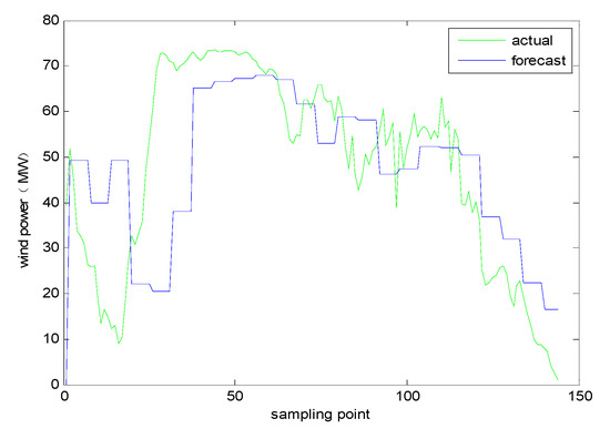
Figure 7.
Power and forecast power of the wind farm.
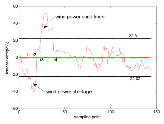
Figure 8.
Power forecast error and the optimal interval.
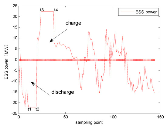
Figure 9.
The charge and discharge of the optimal ESS.
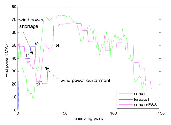
Figure 10.
Wind farm output after compensating error by the ESS.
In Figure 7, Figure 8, Figure 9 and Figure 10, at t1–t2, the forecast error was negative (the actual output of the wind farm was smaller than the forecast output), and ESS discharging was needed. Due to the limitation of rated power of the ESS, not all the forecast error can be completely compensated, there was a certain power shortage in the wind farm, which can be balanced by the purchase of electricity from the grid.
At t3–t4, the forecast error was positive (the actual output of wind farm was larger than the forecast output), and ESS charging was needed. Similarly, due to the limitation of rated power of the ESS, not all the forecast error can be completely compensated and a certain wind curtailment in the wind farm existed.
For the rest times, the actual output of the wind farm after compensation could strictly follow the planned output (forecast output), as shown in Figure 10, the purple curve.
5.5. The Analysis of Influencing Factors on the Optimal Result
About the optimization problem in this paper, we should consider some aspects: in the future, the cost conditions will change; for different purposes, a different compensation degree will be required. Therefore, in this section, we will deeply discuss how these influencing factors affect the optimal result [28,29,30,31,32,33,34,35].
The cost conditions, i.e., the coefficients (C, CP, CE, C1, C2) in Equation (7), included electricity price, ESS unit power cost, ESS unit capacity cost, unit wind curtailment penalty, and unit wind shortage penalty, respectively. In other words, we will discuss how these coefficients affect the optimal result.
5.5.1. The Effect of Electricity Price
Unit electricity price directly affects the profit of the wind farm. The relationship between the max profit and the unit electricity price is shown in Figure 11. The wind farm could be profitable in a certain range of electricity prices. If the price was below a certain lower limit, ESS would not have investment value. Taking 80% error compensation degree as an example, with other factors remaining unchanged, when electricity price was 49.6 $/MWh, the wind farm’s max profit was zero. If below this price, there was no need to invest in ESS. As for other compensation degrees, the corresponding critical prices could also be obtained.
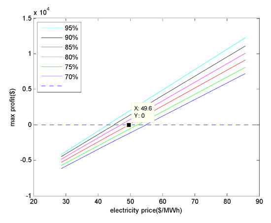
Figure 11.
Relationship between max profit and electricity price.
In Figure 11, at the same compensation degree, with the increase of the unit electricity price, the max profit will increase; while at the same electricity price, with the increase of the compensation degree, the max profit increased. This could be explained by the fact that when the compensation degree increased, the extra generated electricity increased accordingly. On the other hand, the cost of the extra rated power/capacity also increased, which lowered the profit. The overall effects of the two aspects was the increase of the max profit, which was proven by the simulation result.
5.5.2. The Effect of the ESS Unit Cost
The possible change of the unit cost of ESS will affect the optimal result. This section discusses the influence of ESS unit power cost and unit capacity cost on the optimal result in detail.
As shown in Figure 12a, at the same error compensation degree, the max profit decreases with the increase of the ESS unit power cost, which is easy to understand. Under the same ESS unit power cost, if the unit cost was less than a certain value (at the left part of the Figure 12a), the max profit will increase with the increase of the compensation degree, if the unit cost was higher than a certain value (at the right part of Figure 12a), the max profit did not necessarily increase with the increase of compensation degree that the optimal result could appear at a lower compensation degree. This could be explained by that when the ESS unit power cost was too expensive, the more the compensation, the less profit, and even the negative profit.
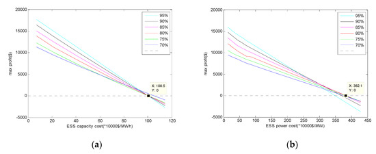
Figure 12.
Relationship between max profit and ESS unit cost: (a) max profit and ESS unit power cost; (b) max profit and ESS unit capacity cost.
Taking 80% compensation degree as an example, when the ESS unit power cost was 382.1 × 10,000 $/MW, the max profit was zero, meaning that above 382.1 × 10,000 $/MW, there would be no need to invest in ESS. For other compensation degrees, the critical ESS unit power cost also could be calculated.
The same as the ESS unit capacity cost (see Figure 12b), the critical unit capacity cost was 100.5 × 10,000 $/MWh at 80% compensation degree.
5.5.3. The Effect of the Compensation Degree
The effect of the compensation degree was related to the ESS unit cost. When the ESS unit cost was below a certain value, the max profit would increase with the increase of the compensation degree, as shown in the left part of the Figure 13; when the ESS unit cost was above a certain value, the max profit did not necessarily increase with the increase of the compensation degree, that the max profit could obtained at a lower compensation degree, as shown in the right part of the Figure 13. This could be explained that if the ESS unit cost is too high, the more compensation, the less profit, even the negative profit.
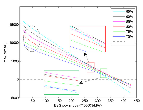
Figure 13.
The effect of the compensation degree on the optimal result.
Exampled in Figure 13, in the ellipse region, the optimal compensation degree was 95%; in the red rectangular region, the optimal compensation degree was 90%; in the green rectangular region, the optimal compensation degree was 85%.
5.5.4. The Effect of the Unit Penalty Cost
As shown in Figure 14, at all error compensation degrees, the higher the unit wind curtailment penalty was, the less the max profit. The max profit value could even go to negative. For example, at 80% error compensation degree, when the unit wind curtailment penalty was larger than 1547 $/MWh, the max profit was negative and thus there was no need to invest in ESS.
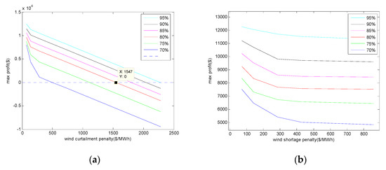
Figure 14.
Relationships between max profit and unit penalty cost. (a) Max profit and unit wind curtailment penalty; (b) max profit and unit wind shortage penalty.
When the compensation degrees were the same, with the increase of the unit wind curtailment penalty, the max profit will decrease.
When the unit wind curtailment penalty was the same, with the increase of the error compensation degree, the max profit increased. This was because with the increase of the error compensation degree, the amount of wind curtailment electricity will decrease, so the total wind curtailment penalty decreased and the max profit increased.
The same relationship was observed for the unit wind shortage penalty and the max profit, as shown in Figure 14b.
5.5.5. Sensitivity Analysis of the Influencing Factors
In order to analyze and compare the influence of these factors quantitatively, a concept of Sensitivity Degree (SD) was introduced.
SD indicates the sensitivity of the evaluation index to each influencing factor. It is defined as dividing the change rate of the evaluation index by the change rate of the influencing factors.
Here,
- index is the max profit;
- parameter is the electricity price (c), ESS unit power cost (cP), and ESS unit capacity cost (cE), unit wind curtailment penalty (c1) or unit wind shortage penalty (c2).
SD > 0 indicates that the evaluation index changes in the same direction as the influencing factors. SD < 0 indicates the opposite change of evaluation index and influencing factors. The larger the | SD | is, the more sensitive the index is to the influencing factor; and vice versa.
For easy comparison, data of the following influencing parameters were normalized: electricity price (c), ESS unit power cost (cP), and ESS unit capacity cost (cE), unit wind curtailment penalty (c1) or unit wind shortage penalty (c2). According to Equation (17), the SD of each influencing parameter was calculated
The sensitivity degrees of these parameters were shown, respectively, in Figure 15. The sensitivity degree of the electricity price was the highest, followed by the sensitivity of ESS unit capacity cost and the sensitivity of ESS unit power cost.
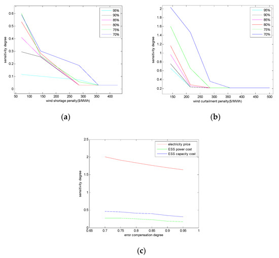
Figure 15.
(a) The sensitivity degree of the electricity price; (b) the sensitivity degree of the wind curtailment penalty; (c) the sensitivity degree of the wind shortage penalty.
As for the sensitivity degree of the unit wind curtailment penalty and unit wind shortage penalty, they varied with the compensation degree, as shown in Figure 15b,c.
When the unit wind curtailment penalty was the same, with the increase of the compensation degree, the sensitivity degree decreased. It could be explained that with the increase of the compensation degree, the amount of the wind curtailment decreased, and thus the effect of the unit wind curtailment to the total profit decreased.
When the compensation degree was the same, with the increase of the unit wind curtailment penalty, the sensitivity degree decreased, and eventually approached to a small constant. It could be explained that when the unit wind curtailment penalty was too large, the optimal compensation interval would approach an interval that included more positive errors (and even all positive errors), so that there would be very small wind curtailment (and even no wind curtailment). In this way, the impact of the wind curtailment to the max profit would be decreased to a very small value.
Finally, if above a certain value of the unit wind curtailment penalty, all sensitivity degrees decreased to the same small constant. In this case, the optimal compensation interval included the most positive errors and the amount of the wind curtailment was the least.
For the sensitivity degree of unit wind shortage penalty, if above a certain value of the unit wind shortage penalty, all sensitivity degrees decreased to the same small constant and even close to zero. In this case, the optimal compensation interval included the most negative errors and the amount of wind shortage approached a very small quantity.
For the case discussed previously in Section 5, at 80% error compensation degree and under the cost condition described in Section 5.2, the sensitivity degrees were calculated, as shown in Table 3.
Table 3.
The sensitivity degree of each parameter.
The comparison showed that at the cost condition described above, the wind farm’s max profit was most sensitive to the electricity price, followed by wind curtailment penalty, wind shortage penalty, ESS unit capacity cost, and ESS unit power cost.
For other cost conditions and other compensation degrees, we can also obtain the sensitivity degree through the method in Section 5.5.5.
6. Conclusions
Based on the field data of the wind farm, aiming at maximizing the profit of the wind farm, a mathematical model and an optimization method was proposed in this paper for planning the ESS size.
First, at the same error compensation degree, compared with the traditional method, the proposed optimization method in this paper could constantly obtain the optimal ESS sizing and the max profit.
Second, the effects of influencing factors (electricity price, ESS cost, wind penalty cost, and compensation degree) on the optimal result (optimal ESS sizing and max profit) was thoroughly analyzed, and the sensitivity and the critical investment range was also determined.
Finally, this comprehensive work provides a powerful decision-making basis for ESS planning in current and future markets, so that the wind farm can better track the planned output and improve the absorption capacity of the grid to the wind power.
Author Contributions
Conceptualization, X.Y. and X.D.; methodology, X.Y.; software, X.Y.; validation, X.Y. and L.Z.; formal analysis, X.D.; investigation, H.Z.; resources, X.Y.; data curation, X.Y.; writing—original draft preparation, X.Y.; writing—review and editing, S.P.; visualization, S.P.; supervision, H.Z.; project administration, H.Z.
Funding
This research received no external funding.
Conflicts of Interest
The authors declare no conflict of interest.
References
- Zhang, L.; Ye, T.; Xin, Y.; Han, F.; Fan, G. Problems and measures of power grid accommodating large scale wind power. Proc. CSEE 2010, 30, 1–9. [Google Scholar]
- Lu, M.S.; Chang, C.L.; Lee, W.J.; Wang, L. Combining the wind power generation system with energy storage equipment. IEEE Trans. Ind. Appl. 2009, 45, 2109–2118. [Google Scholar]
- Sorensen, P.; Cutululis, N.A.; Vigueras-Rodríguez, A.; Jensen, L.E.; Hjerrild, J.; Donovan, M.H.; Madsen, H. Power fluctuations from large wind farms. IEEE Trans. Power Syst. 2007, 22, 958–965. [Google Scholar] [CrossRef]
- Xiao, J.; Bai, L.; Li, F.; Liang, H.; Wang, C. Sizing of energy storage and diesel generators in an isolated microgrid using discrete Fourier transform (DFT). IEEE Trans. Sustain. Energy 2014, 5, 907–916. [Google Scholar] [CrossRef]
- Zhang, N.; Kang, C.; Kirschen, D.S.; Xia, Q.; Xi, W.; Huang, J.; Zhang, Q. Planning pumped storage capacity for wind power integration. IEEE Trans. Sustain. Energy 2012, 4, 393–401. [Google Scholar] [CrossRef]
- Gangui, Y.A.N.; Xiaodong, F.E.N.G.; Junhui, L.I.; Gang, M.U.; Guoqiang, X.I.E.; Xiaochen, D.O.N.G.; Zhiming, W.A.N.G.; Kai, Y.A.N.G. Optimization of energy storage system capacity for relaxing peak load regulation bottlenecks. Proc. CSEE 2012, 32, 27–35. [Google Scholar]
- Wang, C.; Yu, B.; Xiao, J.; Guo, L. Sizing of energy storage systems for output smoothing of renewable energy systems. Proc. Chin. Soc. Electr. Eng. 2012, 32, 1–8. [Google Scholar]
- Liu, Y.; Du, W.; Xiao, L.; Wang, H.; Cao, J. A Method for Sizing Energy Storage System to Increase Wind Penetration as Limited by Grid Frequency Deviations. IEEE Trans. Power Syst. 2015, 31, 729–737. [Google Scholar] [CrossRef]
- Brekken, T.K.; Yokochi, A.; Von Jouanne, A.; Yen, Z.Z.; Hapke, H.M.; Halamay, D.A. Optimal energy storage sizing and control for wind power applications. IEEE Trans. Sustain. Energy 2010, 2, 69–77. [Google Scholar] [CrossRef]
- Bludszuweit, H.; Domínguez-Navarro, J.A. A probabilistic method for energy storage sizing based on wind power forecast uncertainty. IEEE Trans. Power Syst. 2012, 26, 1651–1658. [Google Scholar] [CrossRef]
- Yan, G.G.; Liu, J.; Cui, Y.; Li, J.; Ge, W.; Ge, Y. Economic evaluation of improving the wind power scheduling scale by energy storage system. Proc. CSEE 2013, 33, 45–52. [Google Scholar]
- Luo, F.; Meng, K.; Dong, Z.Y.; Zheng, Y.; Chen, Y.; Wong, K.P. Coordinated operational planning for wind farm with battery energy storage system. IEEE Trans. Sustain. Energy 2015, 6, 253–262. [Google Scholar] [CrossRef]
- Haessig, P.; Multon, B.; Ahmed, H.B.; Lascaud, S.; Bondon, P. Energy storage sizing for wind power: Impact of the autocorrelation of day-ahead forecast errors. Wind Energy 2015, 18, 43–57. [Google Scholar] [CrossRef]
- Papaefthimiou, S.; Karamanou, E.; Papathanassiou, S.; Papadopoulos, M. Operating policies for wind-pumped storage hybrid power stations in island grids. IET Renew. Power Gener. 2009, 3, 293–307. [Google Scholar] [CrossRef]
- Zidar, M.; Georgilakis, P.S.; Hatziargyriou, N.D.; Capuder, T.; Škrlec, D. Review of energy storage allocation in power distribution networks: Applications, methods and future research. IET Gener. Transm. Distrib. 2016, 10, 645–652. [Google Scholar] [CrossRef]
- Zhao, H.; Wu, Q.; Hu, S.; Xu, H.; Rasmussen, C.N. Review of energy storage system for wind power integration support. Appl. Energy 2015, 137, 545–553. [Google Scholar] [CrossRef]
- Khalid, M. Wind Power Economic Dispatch-Impact of Radial Basis Functional Networks and Battery Energy Storage. IEEE Access 2019, 7, 36819–36832. [Google Scholar] [CrossRef]
- Bludszuweit, H.; Dominguez-Navarro, J.A.; Llombart, A. Statistical analysis of wind power forecast error. IEEE Trans. Power Syst. 2008, 23, 983–991. [Google Scholar] [CrossRef]
- Sideratos, G.; Hatziargyriou, N.D. An advanced statistical method for wind power forecasting. IEEE Trans. Power Syst. 2007, 22, 258–265. [Google Scholar] [CrossRef]
- Chen, C.; Duan, S.; Cai, T.; Liu, B.; Hu, G. Optimal allocation and economic analysis of energy storage system in microgrids. IEEE Trans. Power Electron. 2011, 26, 2762–2773. [Google Scholar] [CrossRef]
- Dui, X.; Zhu, G.; Yao, L. Two-stage optimization of battery energy storage capacity to decrease wind power curtailment in grid-connected wind farms. IEEE Trans. Power Syst. 2018, 33, 3296–3305. [Google Scholar] [CrossRef]
- Li, Q.; Choi, S.S.; Yuan, Y.; Yao, D.L. On the determination of battery energy storage capacity and short-term power dispatch of a wind farm. IEEE Trans. Sustain. Energy 2010, 2, 148–158. [Google Scholar] [CrossRef]
- Liu, F.; Pan, Y.; Liu, H.; Ding, Q.; Li, Q.; Wang, Z. Piecewise exponential distribution model of wind power forecasting error. Autom. Electr. Power Syst. 2013, 37, 14–19. [Google Scholar]
- Zhang, Y.; Wang, J.; Wang, X. Review on probabilistic forecasting of wind power generation. Renew. Sustain. Energy Rev. 2014, 32, 255–270. [Google Scholar] [CrossRef]
- Quintero Pulido, D.; Hoogsteen, G.; ten Kortenaar, M.; Hurink, J.; Hebner, R.; Smit, G. Characterization of Storage Sizing for an Off-Grid House in the US and the Netherlands. Energies 2018, 11, 265. [Google Scholar] [CrossRef]
- Wu, Y.; Hongkun, C.; Kunling, X.; Xin, J.; Chun, L. Optimal capacity allocation of energy storage system considering two times scale scheduling cycles. Power Syst. Prot. Control 2018, 46, 106–133. [Google Scholar]
- Xiaowei, D.; Guiping, Z.; Yanzhang, L. Research on Battery Storage Sizing for Wind Farm Considering Forecast Error. Power Syst. Technol. 2017, 41, 434–439. [Google Scholar]
- Xiang, Y.; Wei, Z.N.; Sun, G.Q.; Sun, Y.H.; Shen, H.P. Life cycle cost based optimal configuration of battery energy storage system in distribution network. Power Syst. Technol. 2015, 39, 265–270. [Google Scholar]
- Wang, W.; Mao, C.; Lu, J.; Wang, D. An energy storage system sizing method for wind power integration. Energies 2013, 6, 3392–3404. [Google Scholar] [CrossRef]
- Müller, N.; Kouro, S.; Zanchetta, P.; Wheeler, P.; Bittner, G.; Girardi, F. Energy Storage Sizing Strategy for Grid-Tied PV Plants under Power Clipping Limitations. Energies 2019, 12, 1812. [Google Scholar] [CrossRef]
- Eyer, J.M.; Schoenung, S.M. Benefit and Cost Framework for Evaluating Modular Energy Storage: A Study for the DOE Energy Storage Systems Program; No. SAND2008-0978; Sandia National Laboratories: Albuquerque, NM, USA, 2008. [Google Scholar]
- Liu, P.; Cai, Z.; Xie, P.; Li, X.; Zhang, Y. A Computationally Efficient Optimization Method for Battery Storage in Grid-connected Microgrids Based on a Power Exchanging Process. Energies 2019, 12, 1512. [Google Scholar] [CrossRef]
- Ingram, A.E. Storage options and sizing for utility scale integration of wind energy plants. In Proceedings of the ASME 2005 International Solar Energy Conference, Orlando, FL, USA, 6–12 August 2008. [Google Scholar]
- Feng, J.; Liang, J.; Zhang, F.; Wang, C.; Sun, B. An optimization calculation method of wind farm energy storage capacity. Autom. Electr. Power Syst. 2013, 37, 90–95. [Google Scholar]
- Liu, J.; Chen, Z.; Xiang, Y. Exploring Economic Criteria for Energy Storage System Sizing. Energies 2019, 12, 2312. [Google Scholar] [CrossRef]
© 2019 by the authors. Licensee MDPI, Basel, Switzerland. This article is an open access article distributed under the terms and conditions of the Creative Commons Attribution (CC BY) license (http://creativecommons.org/licenses/by/4.0/).