Application of Artificial Neural Network for the Optimum Control of HVAC Systems in Double-Skinned Office Buildings

Abstract

Double Skin Façade (DSF) systems have become an alternative to the environmental and energy savings issues. DSF offers thermal buffer areas that can provide benefits to the conditioned spaces in the form of improved comforts and energy savings. There are many studies conducted to resolve issues about the heat captured inside DSF. Various window control strategies and algorithms were introduced to minimize the heat gain of DSF in summer. However, the thermal condition of the DSF causes a time lag between the response time of the Heating, Ventilation, and Air-Conditioning (HVAC) system and cooling loads of zones. This results in more cooling energy supply or sometimes less than required, making the conditioned zones either too cold or warm. It is necessary to operate the HVAC system in consideration of all conditions, i.e., DSF internal conditions and indoor environment, as well as proper DSF window controls. This paper proposes an optimal air supply control for a DSF office building located in a hot and humid climate. An Artificial Neural Network (ANN)-based control was developed and tested for its effectiveness. Results show a 10.5% cooling energy reduction from the DSF building compared to the non-DSF building with the same HVAC control. Additionally, 4.5% more savings were observed when using the ANN-based control.

1. Introduction

There is currently international cooperation for the reduction of greenhouse gases under the paradigm of climate change. The international community also agreed that each country should reduce greenhouse gases to a specific target by 2020 [1]. According to the Energy Outlook 2019, the total carbon dioxide emissions in the US are classified into industrial, transportation, residential, and commercial. More than 50% of the electrical energy currently used in the US is produced via fossil fuels, the largest source of greenhouse gas emissions. Urban areas account for most fossil fuel consumption; in other words, most of the carbon dioxide generated by fossil fuels are generated from the energy use of urban space. Accordingly, considering the combined CO₂ emissions from residential and commercial buildings that make up cities, the construction sector is expected to emit about 40% more carbon dioxide than the transportation sector. Moreover, compared to residential buildings in 2019, commercial buildings have about 10% higher carbon dioxide emissions, which is expected to remain steady and not decrease until 2050. These data stress that measures to reduce greenhouse gas emissions from commercial buildings need priority over residential buildings [2].

The window factor is one of the main factors that increase the building energy consumption due to high U-value and solar heat gain. To solve this issue, many studies have been conducted on high-performance windows, smart windows, and shading systems in both industry and academic fields. Energy reduction through the Double Skin Façade (DSF) system has been verified by previous studies [3,4,5,6,7,8,9,10,11,12,13,14,15,16]. If a DSF system is installed in a building, the building has additional space, and it works as a thermal buffer. Through the thermal buffer, window heat loss is reduced in winter. Window heat loss is calculated by multiplying the U-value of the window, the area of the window, and the temperature differences between indoor and outdoor air. With the installation of the DSF system, the outside condition of the building is changed from the weather condition to the indoor air of the DSF system, which has a higher temperature than outdoor air in winter. Through these temperature differences, window heat loss is reduced with the installation of the DSF system. In summer, on the other hand, window opening control is needed to reduce cooling energy consumption by ventilating the hot air inside the DSF system to the outside [3].

Many researchers have conducted studies related to energy saving through DSF system installation. Yoon et al. analyzed heating energy savings by the installation of the DSF system in a high-rise apartment at different floor levels in Seoul, which is a heating dominant area. Results show that the first-floor apartment unit consumes the least heating energy, and the 25th floor consumes the most [4]. Joe et al. analyzed the impact of the DSF design, regarding glazing type and depth of the cavity, on the energy consumption of adjacent conditioned zones. The model in which the optimal DSF design is applied resulted in a 5.62% reduction in energy consumption [5]. Kim et al. conducted the simulation study about thermal and daylighting effects of the DSF system with interior and exterior blinds in Daejeon, South Korea, with the latitude of 36°21′ N and longitude of 127°23′ E. Results showed that the DSF system could save up to 40% for heating load, 2% for cooling load, and 5% for total loads compared to the base model. Also, the DSF system and the exterior blind models could potentially reduce the thermal loads and lighting energy consumption by around 27%–52% [6]. Shameri et al. argued that many experts widely agree that the DSF system is more cost-effective in the long run. Because it is long-lasting and more durable than a single glass facade, it is argued that the DSF system has great potential to reduce energy consumption in a wide range of research areas [7]. Raji et al. aimed to find energy-saving solutions for the envelope design of high-rise office buildings in the Netherlands climates. They selected glazing type, window-to-wall ratio, sun shading, and roofs for the energy saving solutions. They resulted in a high-performance envelope design that offers considerable energy-savings by around 42% for total energy use, 64% for heating, and 34% for electric lighting [8]. Joe et al. conducted an experimental study about the actual thermal behavior of a multi-story DSF in South Korea. The results showed savings of 15.8% for heating energy and 7.2% for cooling energy compared to the single skin facade [9].

Choi et al. measured the actual behavior of a multi-story DSF during the heating season in an office building. They found that significant energy savings are possible if the multi-story DSF is integrated with an HVAC system as a preheating space [10]. Chan et al. reported the findings on the energy performance of DSF applied to the office building in Hong Kong. The results showed that the DSF system with single clear glazing as the inner pane and double reflective glazing as the outer pane could save around 26% in building cooling energy, as compared to a single skin facade with single absorptive glazing [11]. Hamza Neveen compared the performance of the reflective DSF to a single skin façade. The DSF was predicted to decrease total annual cooling loads by approximately 30% in annual cooling loads [12]. Souza et al. compared temperature differences between outside air temperature, indoor air temperature, and temperature of the DSF system. The main result was that the DSF system had a positive effect on the indoor air temperature due to captured heat inside of the DSF system [13]. Zomorodian and Tahsildoost applied the DSF system with louver system to the office building to reduce the energy consumption of an office building in Teheran, Iran. They argued that the DSF system could reduce 14.8% of total building energy compared to the single-layer window system [14]. Gratia and Herde analyzed heating and cooling energy depending on the installed direction of the DSF. The cooling load was increased regardless of the installed direction of the DSF system even though the heating load was decreased [15]. Gelesz and Reith argued that the DSF system could reduce up to 12% of cooling energy in Central Europe, compared to the triple glazing system [16].

The previous studies related to the DSF window control are as follows. Moon et al. proposed a control method to improve indoor thermal comfort and energy efficiency in buildings equipped with the DSF system [17]. Moon et al. investigated the optimal control strategies to maintain the indoor thermal environment and improve energy efficiency based on the ANN-based control [18]. Moon et al. proposed an ANN-based thermal control method for the DSF system in winter [19]. Moon et al. investigated various thermal control algorithms for DSF windows opening cooling systems of buildings in summer. The fuzzy logic-based control algorithm can improve up to 49.4% of building energy efficiency, compared to other algorithms [20]. Moon proposed a control method that can provide an appropriate indoor thermal comfort through the ANN-based control of the cooling system and the DSF windows [21]. Moon et al. used the ANN model to investigate the thermal performance of buildings with the DSF system under various window opening conditions [22]. Alberto et al. suggested that the essential variable of the DSF system is the airflow path [23].

Most previous studies have analyzed that the installation of the DSF system can save the heating and cooling energy; however, there are only a few studies that deal with heating and cooling energy savings through the installation of the DSF system in terms of the optimal control of HVAC systems.

The air temperature inside of the DSF system is changed because of the weather condition, such as air temperature, diffused solar radiation, and direct solar radiation changes in real-time. The air temperature inside of the DSF system affects the indoor heating and cooling loads, which result in a time lag of the HVAC system and indoor thermal conditions. Due to the time lag of the HVAC system and the thermal condition of the space, over operating and under operating occur out of the set-point temperature ranges [17,18,19,20,21,22]. Therefore, if the HVAC system is operated without considering the indoor thermal environment changes due to the thermal buffer, there is a possibility that the cooling and heating energy savings by the installation of the DSF system will be lower than expected. Therefore, to maximize the physical benefits of the DSF system, which is the building energy savings, every variable, constraint, and cooling and heating loads that change due to DSF’s thermal buffer must be accurately predicted and reflected in the HVAC system for optimal control.

However, the existing temperature-based on/off control method for an HVAC system, which is a conventional HVAC system control method, has difficulty in estimating the future state of the system by considering all variables and accurately reflecting it in actual measurement or simulation [24,25,26].

For the future predictive control described above, HVAC system control based on the ANN, which is increasing in application to solve complex problems in various fields, is needed.

The ANN has the ability to learn and analyze mapping relationships, including non-linear phenomena [24,25,26]. In addition, ANN enables more accurate prediction than the mathematical model through adaptability to external changes and enables accurate and efficient control based on this [26].

The main goal of this study is to predict the cooling load changes with the installation of the DSF system and to achieve cooling energy savings through optimal HVAC system controls. To predict the cooling loads, an ANN-based load prediction model is established using the Python program. An office building simulation model, which is based on ASHRAE Standard 90.1-2004, and a DSF system, which has been validated in the previous study, are developed by using the EnergyPlus simulation program.

This study analyzes and compares the cooling energy consumptions between an ANN-based load prediction control and a conventional temperature fixed control. This study also proposes the optimal HVAC control method for an office building that has a DSF system installed.

2. Simulation Modeling

2.1. Simulation Program

This study used two software programs: EnergyPlus to build the simulation model and Python to develop an ANN model. EnergyPlus is a simulation program developed by the US Department of Energy; it combines the merits of Building Loads and System Thermodynamics (BLAST) in the load analysis part and the advantages of DOE-2 in the systems analysis part [27]. In addition, the EnergyPlus simulation program uses the heat balance calculation, which is recommended by ASHRAE; it also has the advantage of dynamic analysis of radiative, thermal conduction and convective heat transfer under an unsteady state. EnergyPlus can perform simulation analysis based on an integrated heat and mass balance that cannot be implemented in existing simulation programs [26,28,29]. Meanwhile, Python is an interpreted language developed by Amsterdam’s Guido Van Rossum in 1990. Python is used across the entire spectrum of social computing, including web programming, numerical computation, data analysis, object-oriented programming, Graphical User Interface (GUI) programming, system utility building, and software development [26,30].

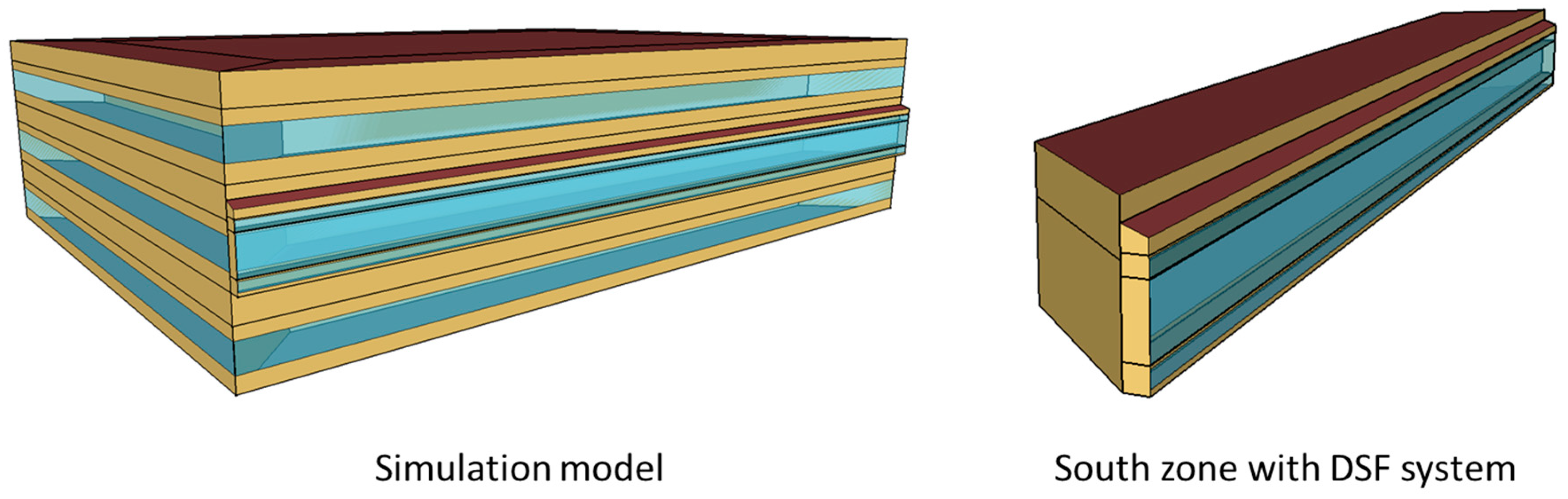
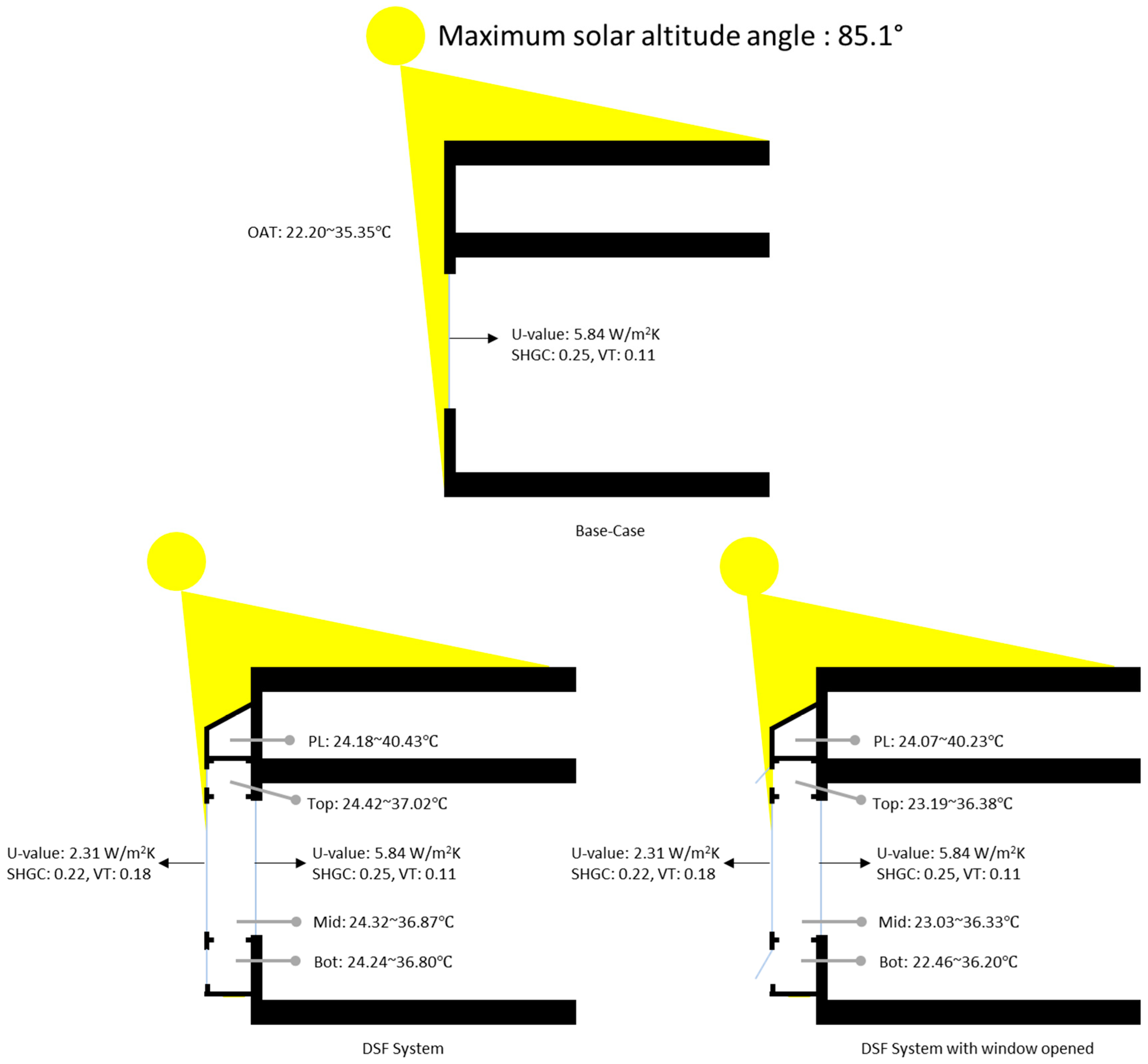
2.2. Simulation Model

The simulation model was implemented using the EnergyPlus simulation program. The left side of Figure 1 shows the large office building simulation model. The size of each floor of the building is 50 × 35 m (1750 m²), and the floor-to-floor height is 4 m. The three-story office building has a 50% window-to-wall ratio (WWR). The size of the south zone, which is attached to the DSF system, is 45.5 × 4.5 m (204.75 m²) and is shown on the right side of Figure 1. Air wall is used for the interior wall between the interior zone and exterior zone for simulation modeling and between exterior zones to divide a thermal zone.

To attach the DSF system to the base model, this paper selected the DSF system that has been calibrated in the previous study [6]. This study only attached the DSF system to the second floor, which is minimally affected by outdoor conditions. To determine how much cooling energy consumption can be saved with the installation of the DSF system, this paper only considered the south zone of the building to which the DSF system is attached. Moreover, to reduce cooling energy consumption, window opening control is necessary to vent out high-temperature air inside the DSF system. Two input parameters are necessary for proper window opening control: first, leakage values, and second, the window opening control schedule. For leakage values, we followed ASHRAE’s leakage values, which is 2.4 cm²/m² for reference office room [6,31]. For the leakage values of the DSF system, we followed the same values used in the previous study [6]. The leakage value for walls without windows was set at 2.6 and at 4.1 cm²/m² for walls with windows [6,32].

The DSF system is constructed as four zones to simulate airflows driven by buoyancy and wind pressure. The top zone of the DSF system is represented as a plenum zone. Horizontal openings are used for each horizontal surface between stacked zones within the DSF system. In this study, vertical opening is controlled by an open and close schedule. The vertical opening schedule is the same as the schedule used in the previous study [6] to simulate the DSF system. The vertical windows, which are located on the bottom and top of the DSF system, are opened when the inside air temperature of the DSF system is higher than the outdoor air temperature, if lower than the outdoor air temperature, then windows are closed. Discharge coefficient values Cd for the window opening are set to 0.65 and 0.2 for vertical and horizontal openings, respectively; these values were obtained from references [33,34].

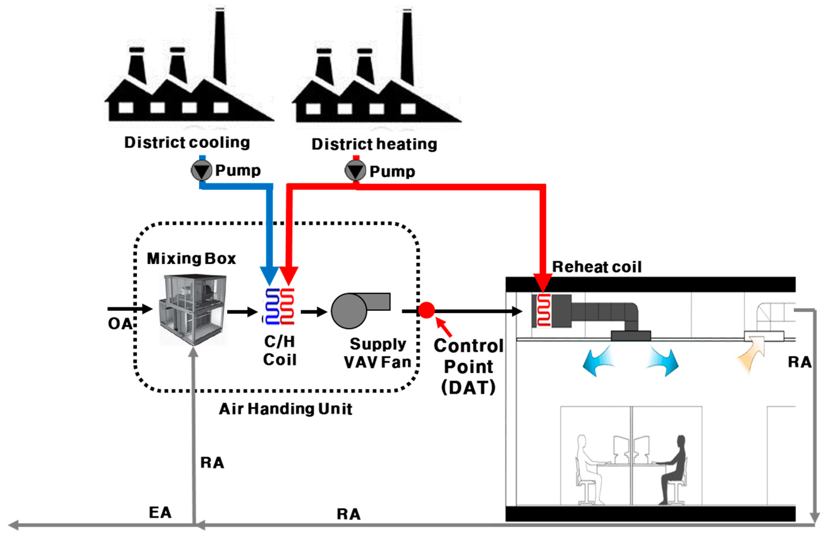
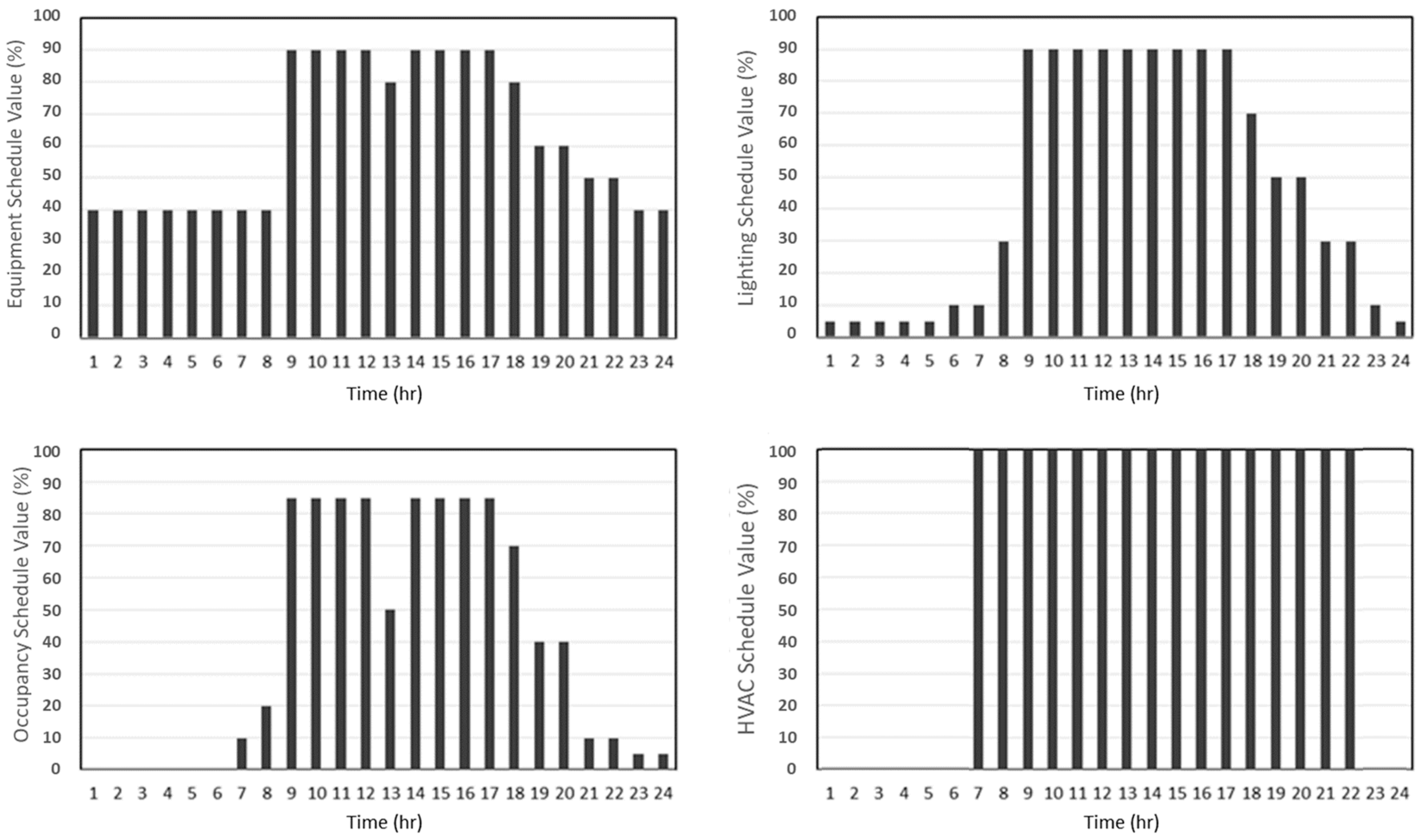
2.3. Simulation Conditions

For this study, a double-glazed window was selected; it consists of 6 mm clear glass, 13 mm air, and 6 mm clear glass. The frame is an aluminum window frame with a thickness of 0.0572 m and a projection length of 0.0254 m from the glass window. The construction and material properties of the simulation model are shown in

Table 1. Construction Properties.

Construction	U-Value (W/m2)	Visible Transmittance	Solar Heat Gain Coefficient	Reference
Exterior Wall	0.79	X	X	ASHRAE Standard 90.1-2004 (Climate Zone 1A)
Interior Wall	5.68	X	X
Raised Floor	1.74	X	X
Ceiling Slab	1.88	X	X
Roof	0.38	X	X
Exterior window for the building	5.84	0.11	0.25
DSF Frame	6.64	X	X	[6]
Exterior window for the DSF system	2.31	0.18	0.22

. Information on the window, exterior wall, interior wall, floor, ceiling, and roof are based on ASHRAE Standard 90.1-2004 Climate Zone 1A, where it is hot and humid. The representative city is Miami, Florida, and the information on the DSF structure, such as the frame of the DSF system and the exterior window of the DSF system, are based on the previous study to construct the same DSF system as in the previous study [6]. The zone cooling set-point temperature is at 24 °C in occupied hours.

The conditions of internal heat gain are shown in

Table 2. Indoor condition.

Type	Input
People	0.057 Person/m2
Light	11.840 W/m2
Equipment	10.333 W/m2
Cooling set-point temperature	24 °C

. Figure 2 shows the schedules of occupants, lights, and equipment during weekdays, which are based on the ASHRAE Standard 90.1-2004. The HVAC system operates from 07:00 to 22:00 on weekdays.

The HVAC system of the simulation model is an Air Handling Unit (AHU)-based conventional HVAC system that consists of a hot water coil and a reheat coil receiving hot water from the district heating system and a cooling coil receiving chilled water from the district cooling system, as shown in Figure 3. The ideal load system is assigned to the building except for the south zone. The OA, RA, and EA refer to outdoor air, return air, and exhaust air in Figure 3. The AHU consists of a mixing box, cooling coil, heating coil, and supply fan. The control point in this study is located after the supply variable air volume fan, which is called AHU discharge air.

2.4. Three Simulation Cases

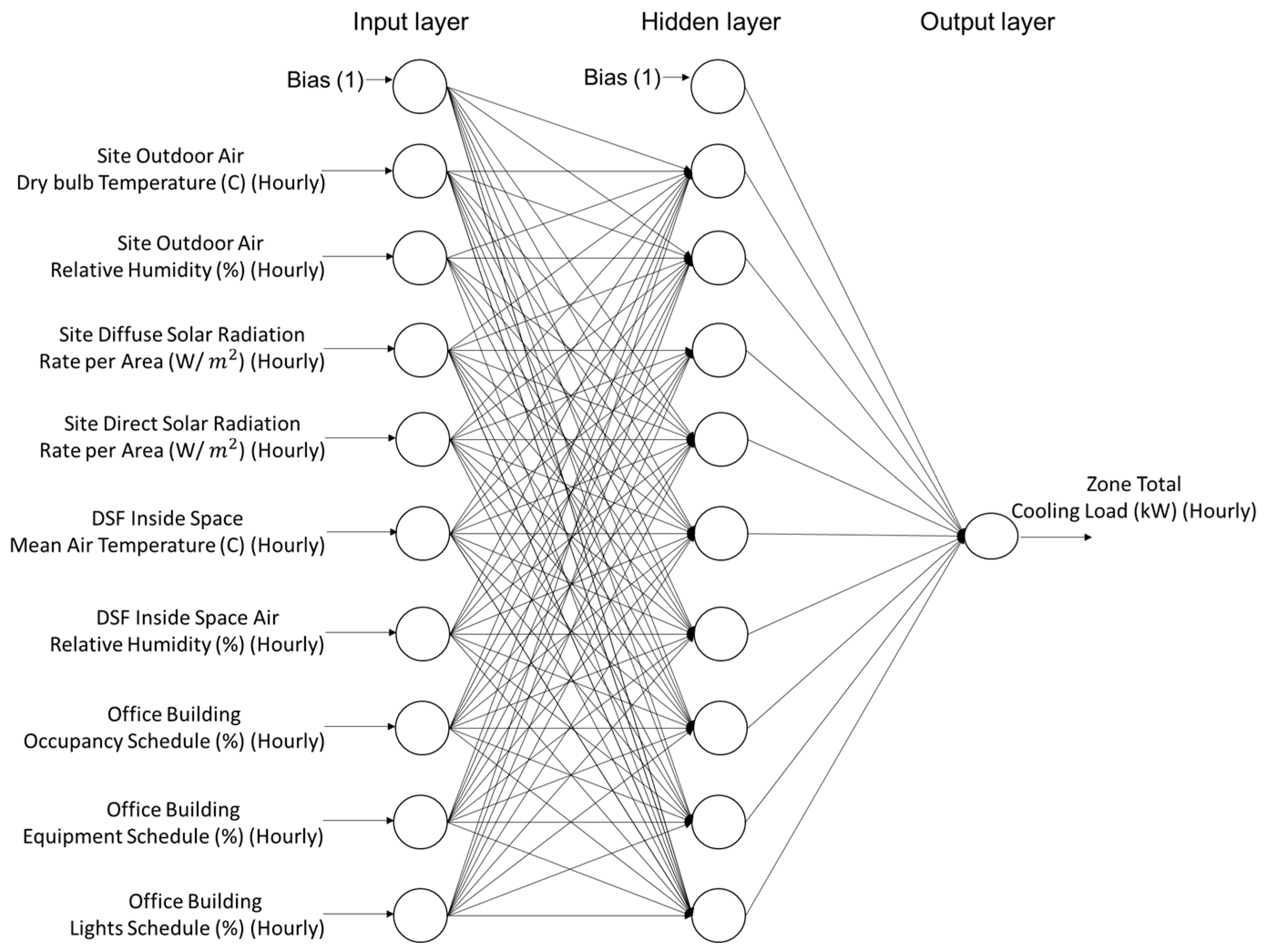
There are three simulation cases developed. Case 1 is the base case, which does not have the DSF system in the building and has a fixed AHU discharge air temperature. To determine the physical advantage of a DSF system, Case 2 has a DSF system attached to Case 1 and has an AHU discharge air temperature. For the proposed ANN-based HVAC system control, Case 3 applies ANN-based HVAC system control to Case 2. By comparing Case 1 and Case 2, the cooling energy savings due to the DSF installation can be analyzed. Meanwhile, by comparing Case 2 and Case 3, the additional cooling energy savings due to the ANN-based HVAC system control can be analyzed.

2.5. ANN Modeling

In this study, we developed an ANN model using Numerical Python (NumPy) and Scientific Python (SciPy) libraries of Python in the same way as previous studies [26].

When designing the ANN model, it is essential to select the activate function depending on the application. The activate function is used to simulate the behavior of biological neurons. In this paper, we used the sigmoid function, which is commonly used for various activate functions. The sigmoid function calculates the result value between 0.00 and 1.00. The sigmoid function is used for non-linearly separable problems, such as load predictions and energy consumption predictions [18,19,20,21,22,26].

Before making the ANN model, the learning method should also be determined. This study used supervised learning, one of the learning methods commonly used in ANN-based prediction models. Supervised learning requires both “input” and “correct answer” datasets. “Correct answer” datasets are result values given to the ANN model. They are used to determine the reliability of the predicted or calculated result data from the input datasets given to the ANN model. In the case of a model for predicting cooling loads, input datasets consist of the outdoor dry bulb temperature, outdoor relative humidity, and solar radiation; in the ANN model, outputs are the predicted cooling loads. The learning process in supervised learning consists of updating the weight factors so that error is reduced by comparing the output values of the ANN model with the “correct answer” values. Therefore, when specific datasets are input, the ANN model, which has learned via supervised learning, processes the patterns of the input values and generates the calculated results, which are determined to be closest to “correct answer” datasets. In addition, each neuron is connected by weight factors. Each neuron adds the product of the input values and the weight factors that are connected and passes this value to the input value of the activate function. If the input values passed onto the previously calculated activate function are not large enough to exceed a certain threshold, it will not output anything. Conversely, if the input value given to the active function exceeds the threshold, the neuron is activated to transmit the data to the next step. Accordingly, ANN computes the results by analyzing the interaction between data, weight factors, and activate function [21,26].

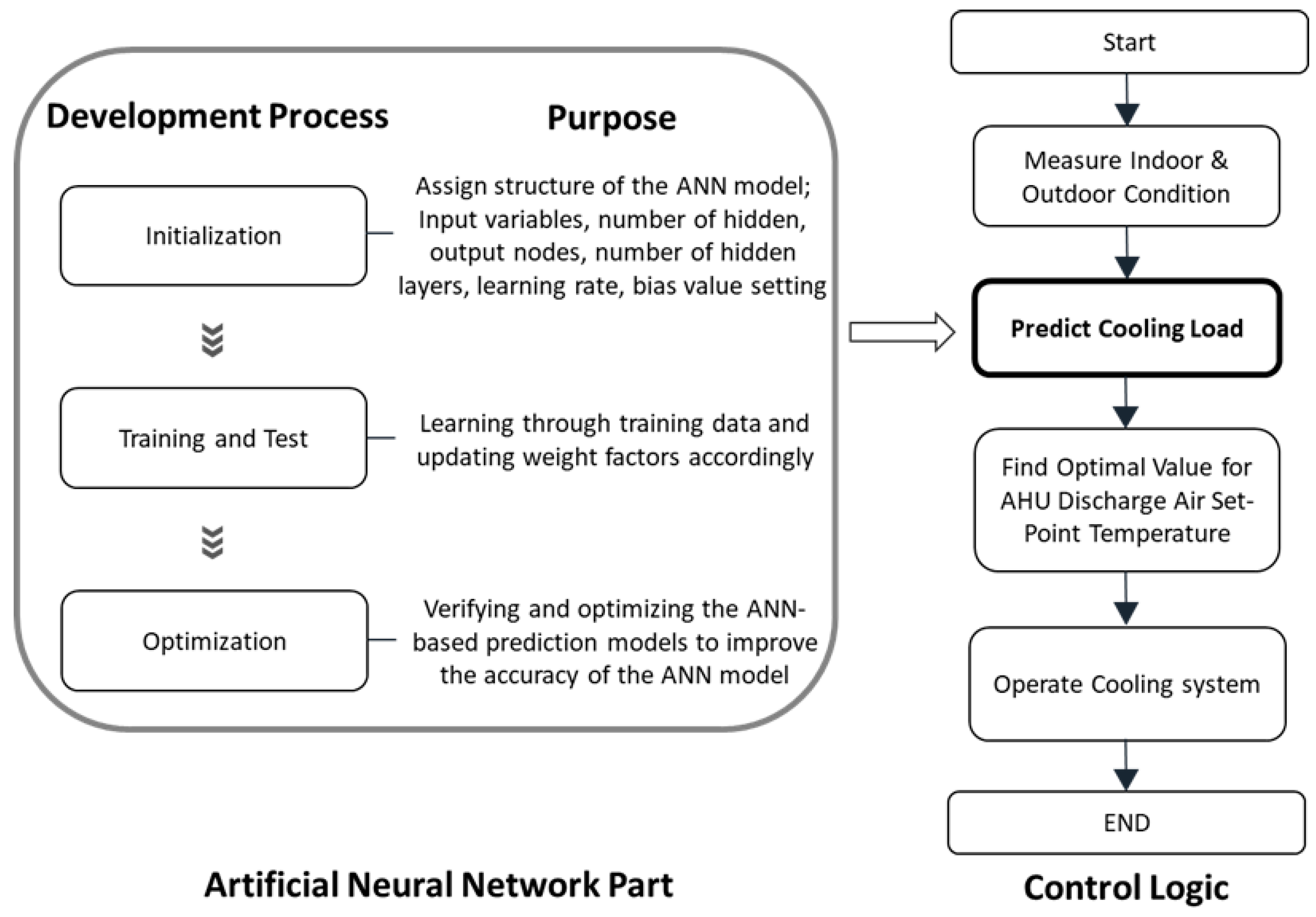
2.6. Development Process of the Predictive ANN Model

The predictive ANN model has two different parts: the ANN part and the control logic part. The ANN part consists of three steps, as shown on the left side of Figure 4 [26]. The purpose of the ANN part is to predict output datasets.

The first step in predicting output datasets is selecting variables that are highly correlated with the output to be predicted. The correlation analysis of variables is needed to select the variables through objective indicators, and correlation analysis can be increased by the efficiency of training. Input variables are selected with a relatively high correlation by analyzing ${\mathrm{r}}^2$, which represents the correlation between all the computable input variables and the output variable [24,25,26,35].

The second step is training and testing. Initializing the weight factors, which is the heart of learning, is the starting point of training. Then, the sum of the values obtained by multiplying the input data by the weights is added to each node and bias. This value is input into the activate function to output values [24,25,26,35]. The error rate between the result of the ANN and the “correct answer” is reflected in the next training, and the training is repeated to reduce the error rate by the epoch value. Epoch represents the number of training repetitions. As mentioned above, the goal of learning is to get the weight factors that have the lowest error rate between the output of the ANN and the “correct answer”. Unlike the previous learning part, the test process does not adjust the weight factors based on the error rate between the ANN results and the “correct answer”; nonetheless, it confirms the predicted accuracy rate of the ANN model that has been trained.

The last step is optimization. The optimization of ANN means adjusting hyper-parameters of the ANN model, such as the bias value, the learning rate, the number of hidden neurons, and the number of hidden layers. The purpose of optimization is to verify the predictive performance and reliability of the ANN model. To confirm this, the statistical term or the coefficient of variance of the root mean square error (CVRMSE) is used in conjunction with the tolerance range proposed in the American Society of Heating, Refrigerating, and Air-Conditioning Engineers (ASHRAE) Guideline 14. The tolerance ranges (or error rates) pertain to the prediction accuracy of the result of the ANN model compared to the result of the EnergyPlus data. The closer the CVRMSE value is to 0%, the better prediction performance is. The ASHRAE recommends a CVRMSE value of less than 30% as the error rate tolerance of time data. This value includes the recommended r² value of 0.80 or higher to indicate correlation [35]. If the CVRMSE value exceeds 30%, the user repeats a series of operations to adjust the hyper-parameter values and performs the optimization process until the tolerance value is less than 30% or reaches a certain value (or goal). Equations (1) and (2) show the calculation formulas of RMSE and CVRMSE, respectively [24].

The control logic part consists of four steps, as shown on the right side of Figure 4. The first step of the control logic part is gathering indoor and outdoor condition data through experiments or simulation models.

The second step of the control logic part is predicting the output through the input datasets, and this step is connected to the ANN part. In this study, the output datasets are the cooling loads. The third step is finding the optimal value for the controlled parameters to achieve control after finishing the optimization process. In this paper, the AHU discharge air set-point temperature is the controlled parameter to save on cooling energy consumption. The final step is operating a cooling system using an optimal controlled parameter.

$$RMSE= \sqrt{\frac{{\displaystyle \sum }{\left(S-M\right)}_{interval}^2}{N_{interval}}},$$

(1)

$$CV\left(RMSE\right)= \frac{RMS{E}_{period}}{A_{period}},$$

(2)

$$A_{period}= \sqrt{\frac{{{\displaystyle \sum }}_{period}{M}_{interval}}{N_{interval}}},$$

(3)

where,

S = ANN model prediction value,

M = EnergyPlus simulation results,

N_interval = Number of EnergyPlus results, and

A_period = Measurement period average.

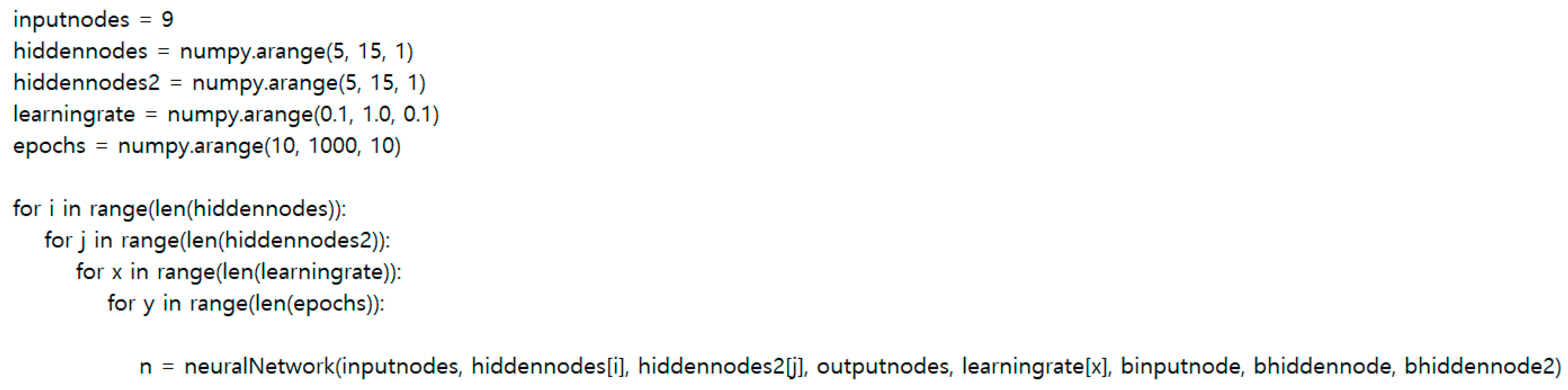
2.6.1. Subsubsection Initial ANN Model Development

The datasets are divided into (1) learning and (2) verification datasets. Training data was only used in the training part, and test data was used in the test part because if the same dataset is used in both the training and test parts, the ANN can predict well for specific conditions, but it may not predict well when a new pattern data is used. We, therefore, implemented the training and testing datasets by randomly dividing the EnergyPlus simulation results at a 9:1 ratio to confirm the ANN’s adaptability to the new patterns that were not experienced in the training part. In addition, input variables were selected using nine variables with relatively high $R^2$ values through correlation analysis with the zone cooling loads as follows: outdoor air dry-bulb temperature, outdoor air relative humidity, site diffuse solar radiation rate per area, direct solar radiation rate per area, DSF inside space mean air temperature, DSF inside space air relative humidity, office building occupancy schedule, office building equipment schedule, and office building lights schedule.

The learning data for the ANN model was built using EnergyPlus. Data, including weekends, from June 1 to August 31, were collected and used. Figure 5 and

Table 3. Initial ANN structure and parameter values.

Division	Range	Initial Values
Number of Hidden Layers	1–n	1
Number of Hidden Neurons	1–n	9
Learning Rate	0.01–1.00	0.2
Epochs	1–n	300

show the structure of the initial cooling load prediction model. The structure of the initial model has nine input nodes, one hidden layer, nine hidden nodes, and one output node. The sigmoid function was used as an activate function. The learning rate was set at 20%, which means that only 20% of the error is used to update the weight factors when an error of 1 occurs. The reason for not fully reflecting 100% of the error is that the optimal weight factors have been set using the gradient descent method. This method has advantages, especially when it has to cope with a function with multiple parameters. This method uses a step-by-step approach to find optimal answers; hence, choosing a learning rate that is too high or too low may not lead to the value that minimizes the error.

Bias is a variable that controls how easily a neuron is activated. Epoch refers to the number of repetitions of learning. For example, when learning is performed with Epoch 100 and 1000 training data, the 1000 × 100 times weight factors update is completed. Compared to the test data, the CVRMSE of the cooling loads predicted by the ANN model was 20.34%, which is within the acceptable tolerance range of 30% recommended in the ASHRAE Guideline 14.

2.6.2. Subsubsection Initial ANN Model Development Optimized Performance Analysis of the ANN Model

ANN model optimization refers to the process of finding optimal learning rates, hidden nodes, hidden layers, and epochs to optimize prediction performance. There are no known steps to determine the values of a hyper-parameter for any problem. Currently, the best approach is to check the results and adjust the learning rate, hidden nodes, hidden layers, and epoch values through trial-and-error processes. The process is repeated until the error rate achieves the acceptable uncertainty ranges proposed in the ASHRAE Guideline 14. In this study, about 100,000 optimization trials were conducted to achieve model optimization. Figure 6 conceptually represents the optimization process conducted to determine the optimal combination in the cooling load predictive algorithm. In the optimization process, the CVRMSE values were compared, and the combination that showed lower CVRMSE was selected.

Figure 7 and Figure 8 show the structure and accuracy rate of the optimized prediction model.

Table 4. Optimal ANN structure and parameter values.

Division	Range	Optimize Values
Number of Hidden Layers	1–n	2
Number of Hidden Neurons Layer 1	1–n	11
Number of Hidden Neurons Layer 2	1–n	9
Learning Rate	0.01–1.00	0.1
Epochs	1–n	800

includes the hyper-parameter values with the lowest CVRMSE and the possible input ranges. After the optimization process, the CVRMSE value decreased to 4.63% from 20.32%. Notably, the error rate in the current model is lower than that of the earlier model. The results indicate that the ANN model developed for load prediction can be used for HVAC optimal control.

2.6.3. Initial ANN Model Development Optimized Performance Analysis of the ANN Model HVAC Control Strategy Based on the ANN Results

The determining method of the AHU discharge air temperature using the ANN-based cooling load prediction model in this study is as follows:

The appropriate AHU discharge air temperature is determined for each hour within the range of 11.11 to 16.67 °C during the daytime, using the linear interpolation formula based on the cooling load predicted by the ANN model when the zone cooling set-point temperature is 24 °C. In addition, the control logic is set such that the AHU discharge air temperature is fixed at 16.67 °C because the cooling load is low during nighttime when the cooling set-point temperature is 26.67 °C.

In summary, during the daytime, when the zone cooling set-point temperature is 24 °C and the cooling load is high, the appropriate AHU discharge air temperature is determined according to the cooling load. During the nighttime, when the cooling set-point temperature is 26.67 °C, the AHU discharge air temperature is fixed at 16.67 °C, regardless of the amount of the cooling load.

3. Results Analysis and Discussions

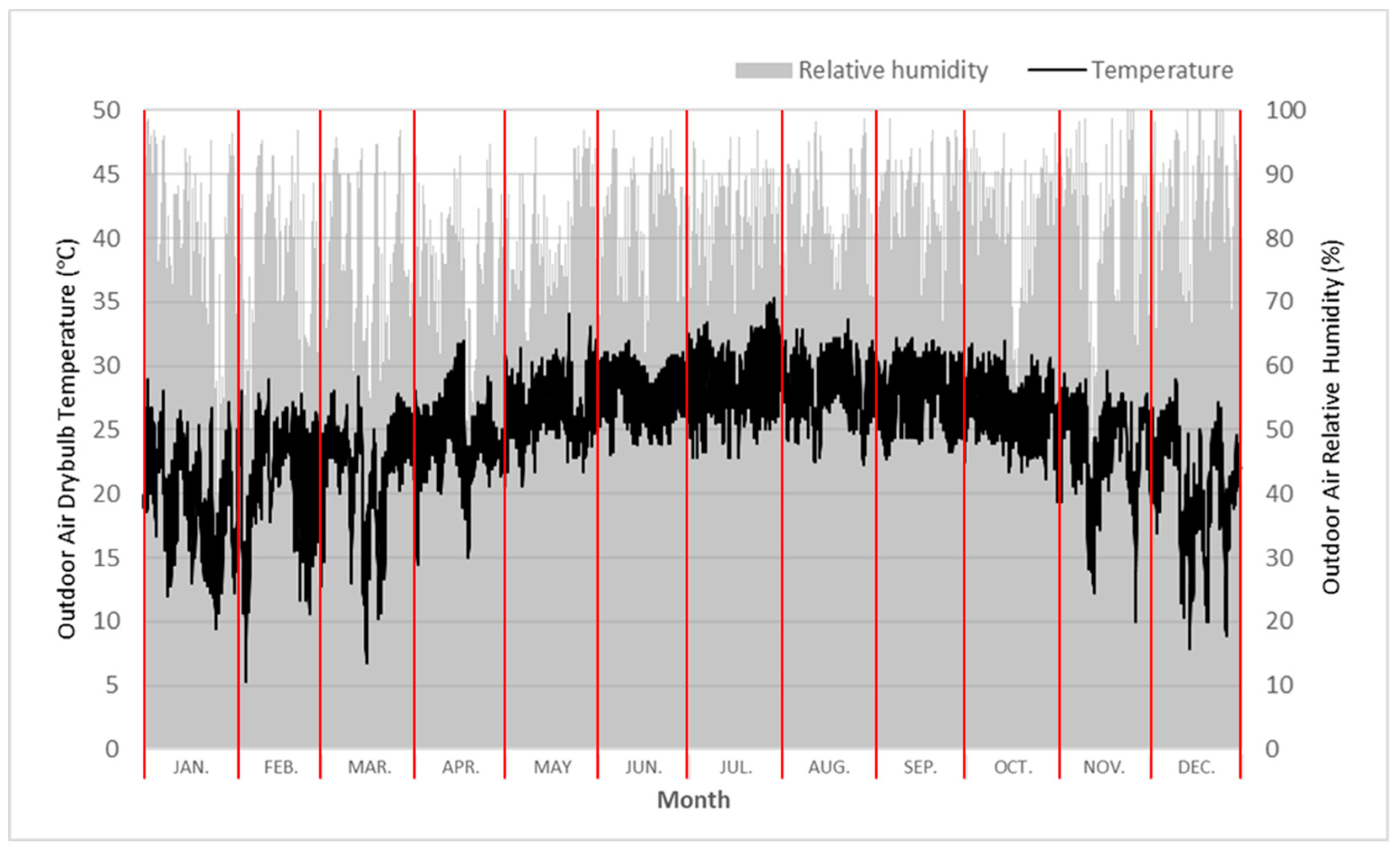
3.1. Weather Conditions

This study used the typical meteorological year (TMY) weather data of Miami, one of the cooling-dominated regions in the US. Figure 9 shows the outdoor air temperature and relative humidity patterns in Miami, Florida. The lowest outdoor air temperature is 5.3 °C, while the highest is 35.35 °C. The lowest relative humidity is 20.42%, and the highest is 100%. The outdoor air temperature range during the summer season, which is between June 1 to August 31, the analysis period in this paper, is 22.2–35.35 °C. The outdoor air relative humidity range during the analysis period is 40.42%–98.75%.

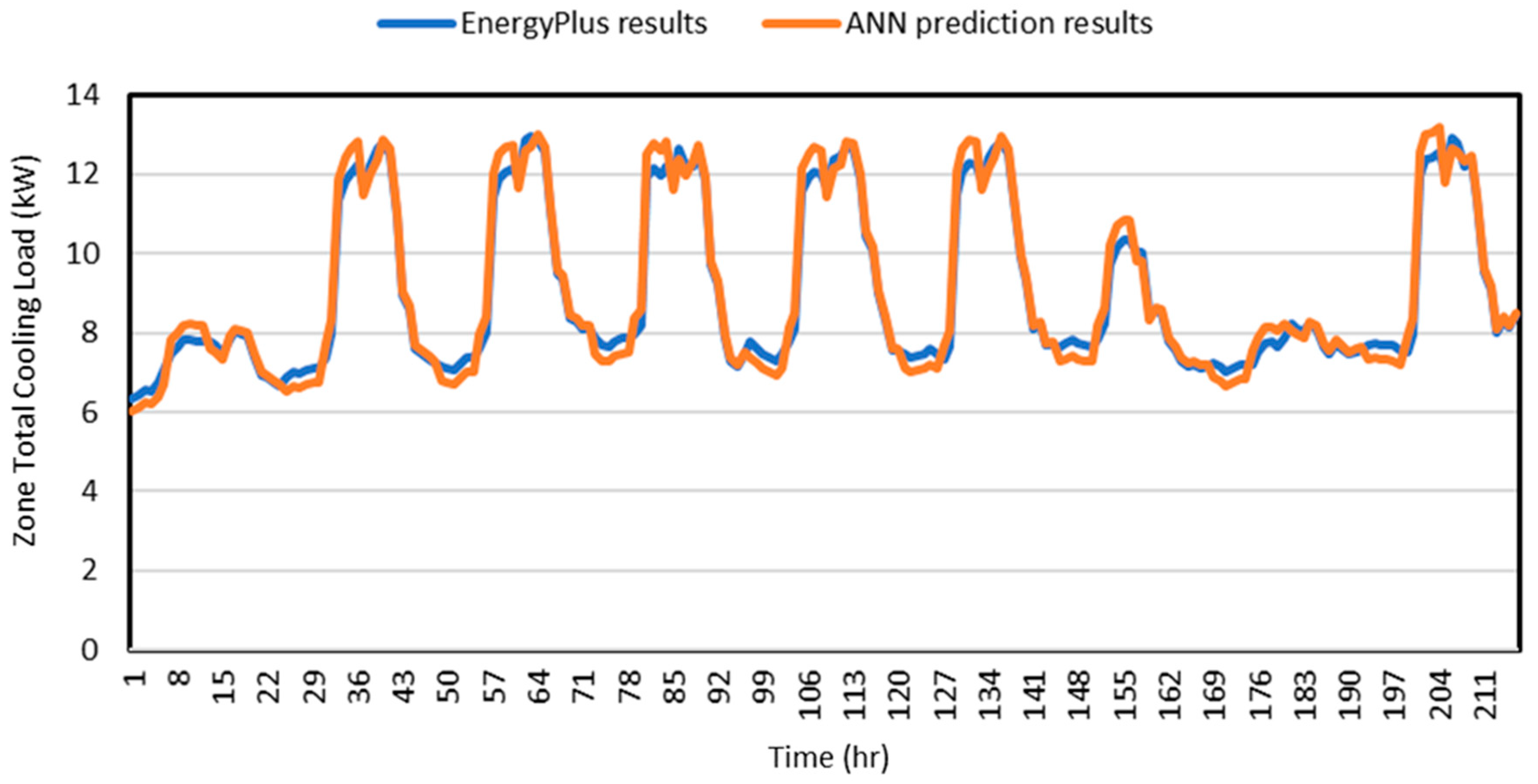
3.2. Analysis of the Summer Representative Day

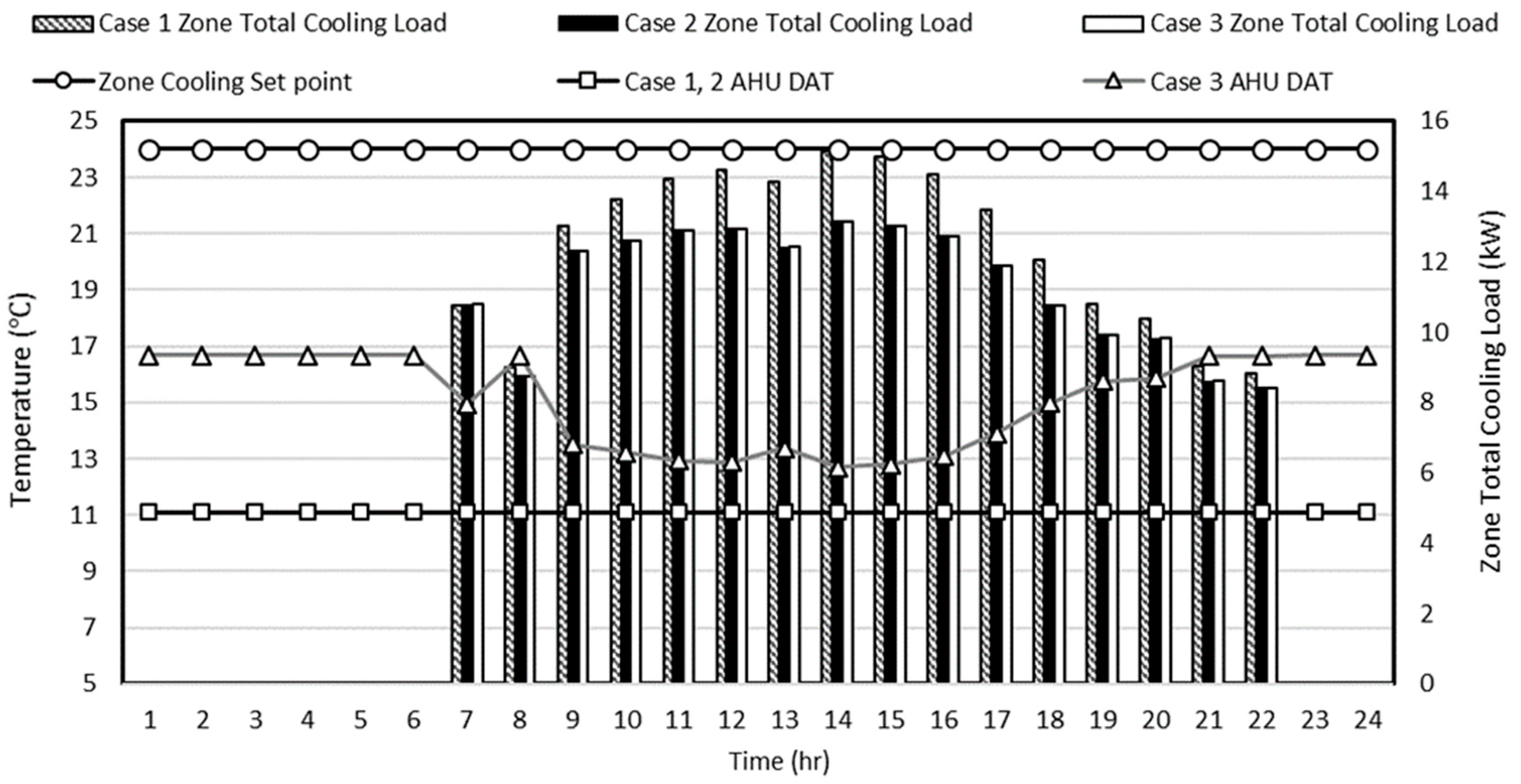
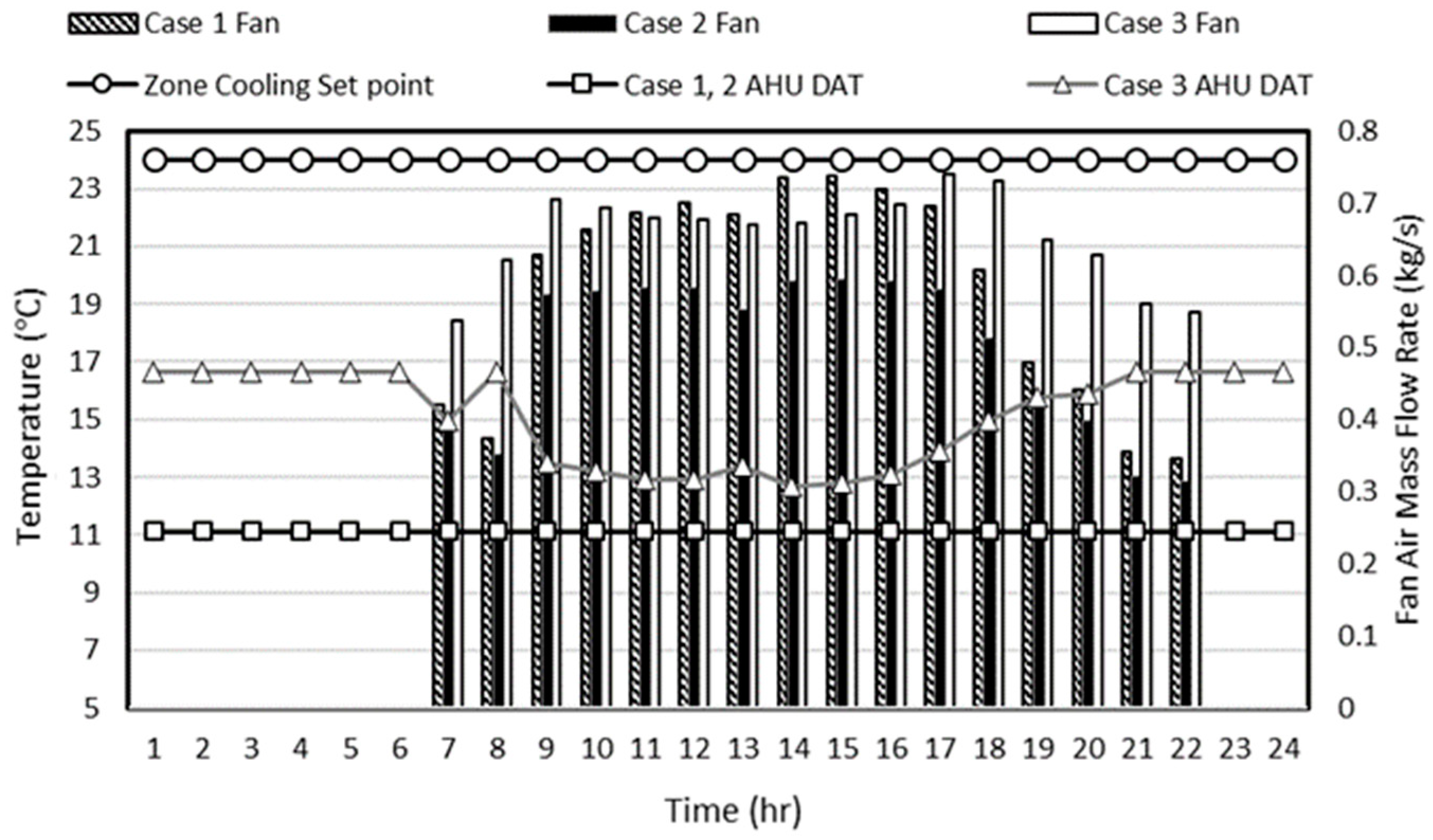
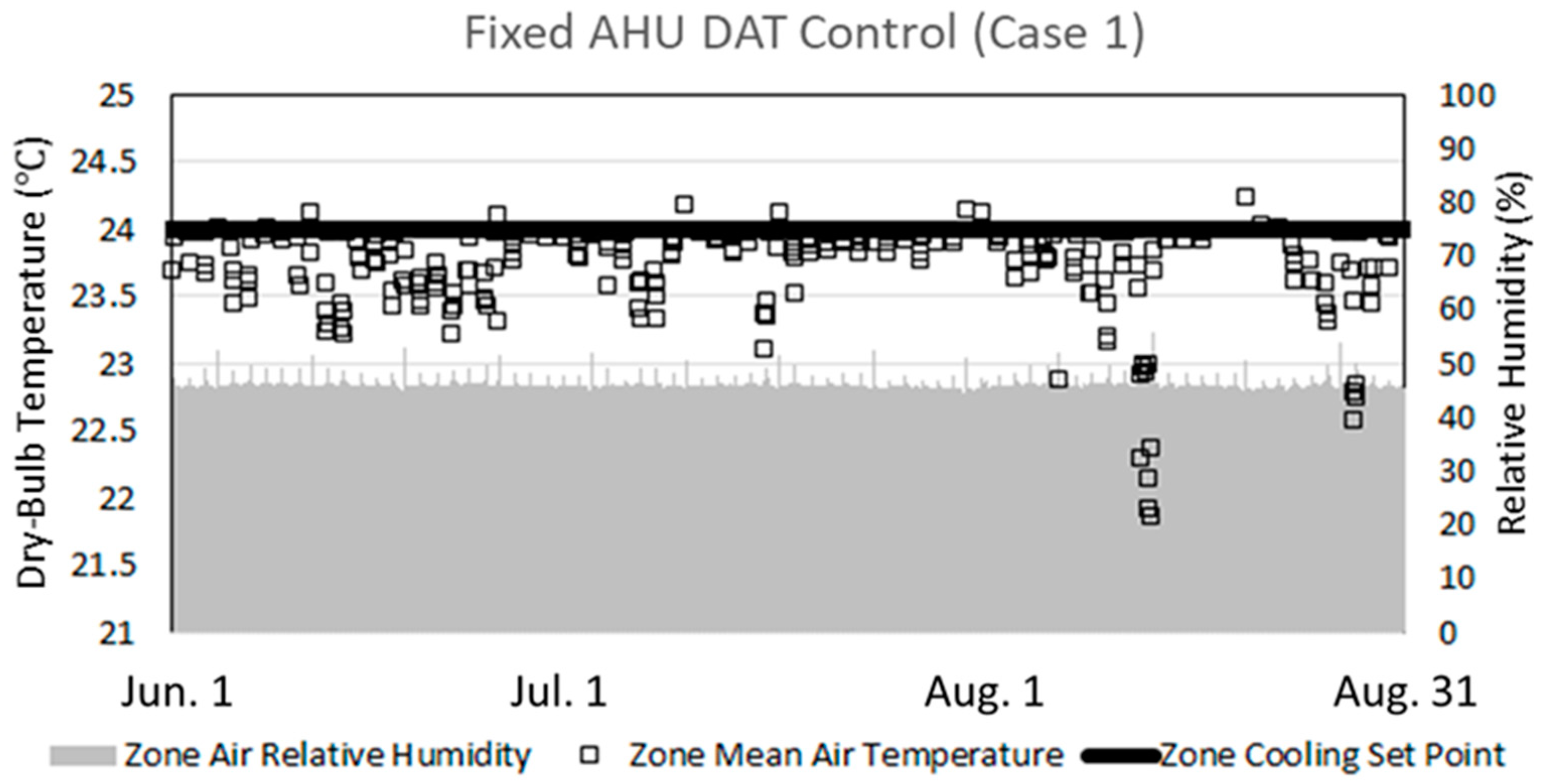
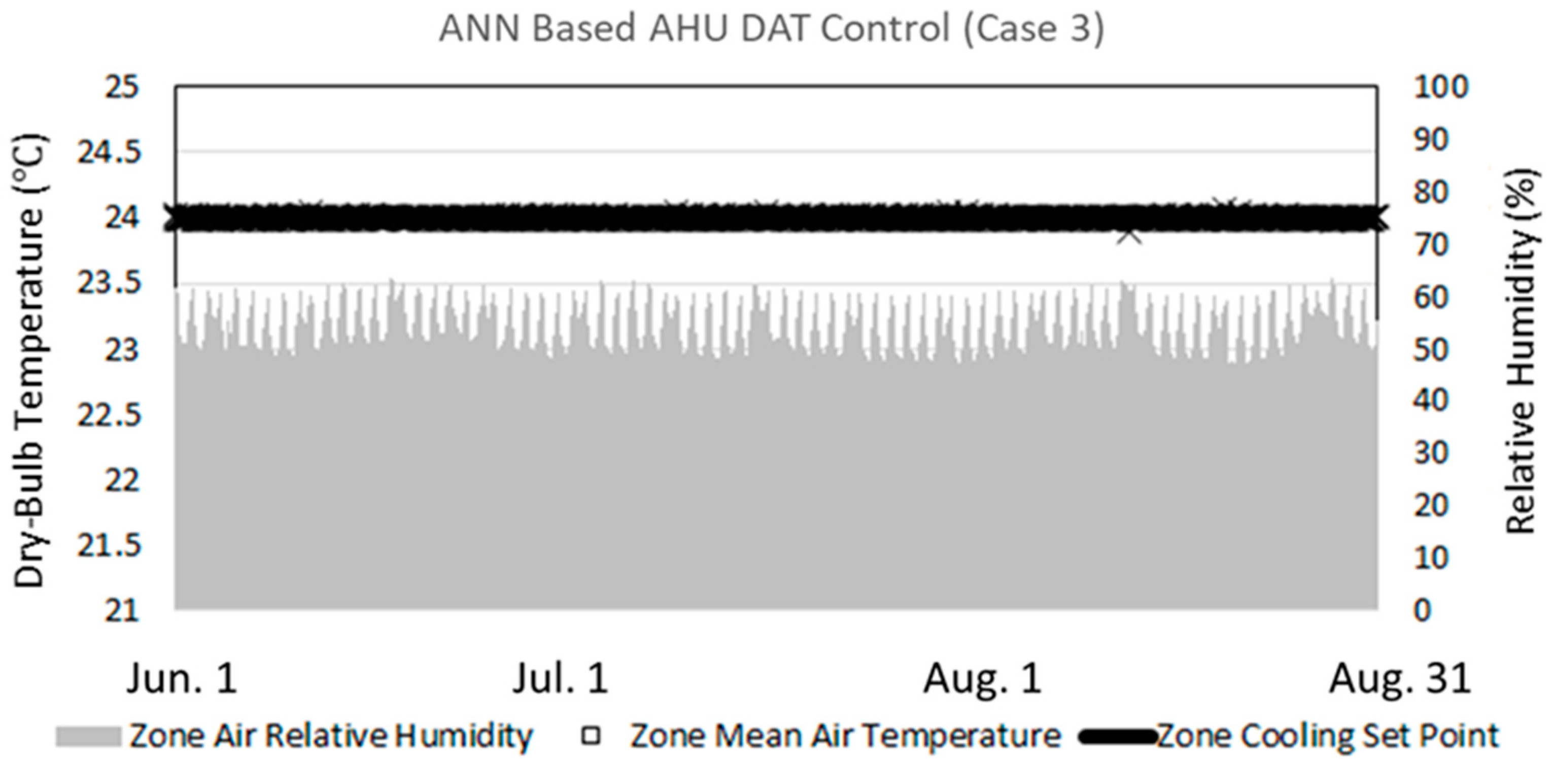
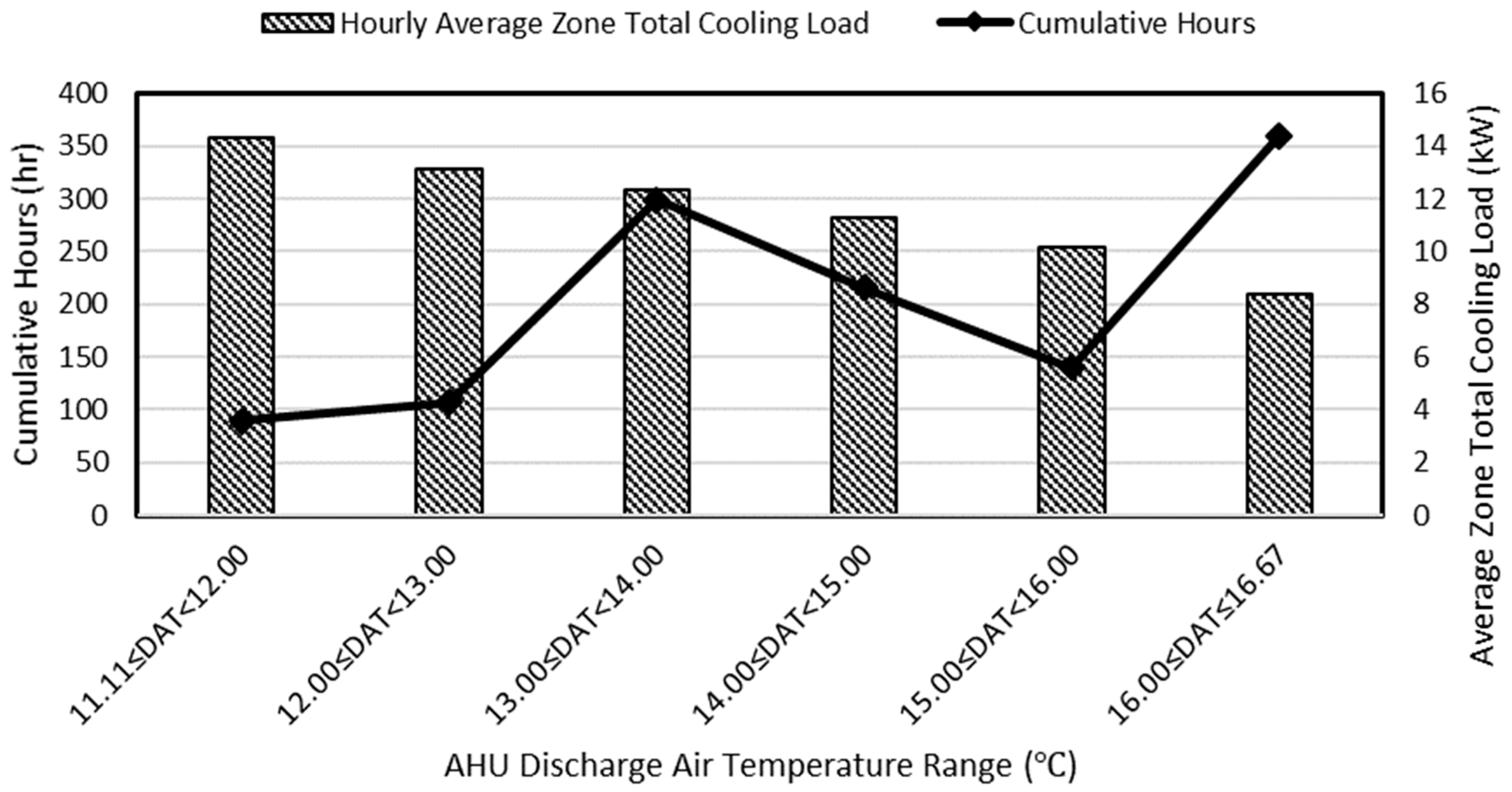
3.2.1. Comparison of AHU Discharge Air Temperature Pattern on the Summer Representative Day

For the summer representative day for this study, 21 July was chosen, which is a summer design day presented in the Miami weather file. Figure 10 shows the change in AHU discharge air temperature according to the cooling loads on the summer representative day. The pattern of the cooling loads on the summer representative day showed similar patterns in all cases, increasing rapidly from 09:00 and gradually decreasing after 17:00. The cooling loads pattern is similar to the pattern of the internal heat gain schedules in Figure 2. The cooling loads at 07:00 are high due to the thermostat set temperature change from the nighttime setback.

The cooling loads in Case 2 and Case 3 are the same because all conditions are the same. Meanwhile, the cooling loads in Case 1 are higher by about 9.0% than those of Case 2 and Case 3. This trend is further described in Section 3.2.2. All three cases have the same zone cooling set-point temperature of 24 °C, and the HVAC system operates from 07:00 to 22:00 on weekdays. However, for the set value of the AHU discharge air temperature, Cases 1 and 2 are fixed at 11.11 °C, regardless of cooling load changes. As described in Section 2.6.3, in Case 2, although the cooling loads and the zone cooling set-point temperatures change, the AHU discharge air temperature is controlled between 11.50 to 15.47 °C from 07:00 to 22:00 by cooling load changes when the HVAC system operates.

Figure 11 shows the window heat gain rate on 21 July. The south zone with the DSF is 50 m in length and 4.5 m in width. The shape of the south zone is narrow and long, as shown in Figure 1. As such, window heat gain rate through the exterior window has a dominant effect on cooling. As previously shown in Table 1, the ASHRAE Standard 90.1-2004 includes a high U-value of 5.84 W/m²K for the exterior window. As a DSF is attached, the U-value of the exterior window is changed from 5.84 to 2.31 W/m²K; a 600-mm air cavity is generated by the DSF added.

One of the main parameters of the window heat gain rate is the solar radiation rate. As solar radiation passes through the exterior window of the DSF, direct solar turns into diffuse solar, and solar heat gain in the zone through the window of Case 2 is considerably lower than that of Case 1 where solar heat gain enters the room directly through the window.

In general, the inside temperature of the DSF system is higher than the outside air temperature in summer, and this can adversely affect cooling energy consumption. Figure 11 can explain this issue.

The Outdoor Air Temperature (OAT) shown in Figure 12 refers to the outside air temperature, while the PL refers to the plenum space of the DSF system. Top, Mid, and Bot represent the temperatures of the top, middle, and bottom spaces of the DSF system, respectively. The inside air temperature of the DSF system increases from bottom to top on the right side of Figure 12; however, the temperature difference is only 0.15 °C. The inside temperature of the DSF system is about 2 °C higher than the outside air temperature. In addition, the temperature range of the plenum space of the DSF system is between 24 to 40 °C in summer; it is higher than the inside air temperature of the DSF system and the outdoor air temperature. This is because the plenum space of the DSF system is directly affected by solar radiation during the summer when the maximum solar altitude angle is 85°. Due to this high solar altitude angle, the roof of the plenum space received solar radiation directly. Because of the plenum space of the DSF system, the inside air temperature of the DSF system is relatively lower than the inside air temperature of the plenum space of the DSF system. In addition, since the plenum space of the DSF system faces the return plenum space of the office building, the high temperature inside the plenum space does not directly affect the conditioned zone.

From these results, it can be seen that the installation of the DSF system reduces cooling energy due to the plenum space of the DSF system and the low window heat gain. In addition, when the exterior windows located at the top and bottom of the DSF system are opened, the inside air temperature of the DSF system is decreased by about 0.6 to 1.8 °C compared to the temperature when windows are closed; this is because the outside air and the inside air of the DSF system are mixed. Therefore, cooling energy is further reduced by opening the exterior windows of the DSF system.

Through these results, the cooling load patterns can be interpreted and are shown in Figure 10. As shown in Figure 12, the inside temperature of the DSF system is higher than the outside air temperature; however, the DSF system prevents solar radiation from reaching the zone directly in the daytime. That is why the cooling loads of Case 2 are lower than that of Case 1.

3.2.2. Comparison of the Fan Mass Flow Rate on the Summer Representative Day

Figure 13 shows the fan mass flow rate change according to AHU discharge air temperature change on the summer representative day. In Case 1, the maximum fan mass flow rate was 0.7373 kg/s at 15:00, and the minimum fan mass flow rate was 0.3450 kg/s at 22:00. In Case 2, the maximum fan mass flow rate was 0.5941 kg/s at 16:00, and the minimum fan mass flow rate was 0.3135 kg/s at 22:00. In Case 3, the maximum fan mass flow rate was 0.7401 kg/s at 17:00, and the minimum fan mass flow rate was 0.5366 kg/s at 07:00.

Comparing the fan mass flow rates of Case 1 and Case 2, Case 2 required 14.3% less fan mass flow rate. Comparing fan mass flow rate between Case 1 and Case 3, Case 3 needed 13.2% more fan mass flow rate than Case 1. In Case 1 and Case 2, the cooling set-point temperature and AHU discharge air temperature are fixed, regardless of the change in cooling loads. The cooling loads are covered by increasing or decreasing the fan mass flow rate. Case 1 has a higher fan flow rate than that of Case 2 and Case 3 because Case 1 had relatively higher cooling loads than the other two cases during the summer representative day. However, in Case 3, the temperature difference between the zone cooling set-point temperature and the AHU discharge air temperature continuously changes based on the cooling loads, and the fan mass flow rate is also increased or decreased to cover the cooling loads.

In summary, the AHU discharge air setpoint temperatures in Cases 2 and 3 are different even though both cases have the same cooling loads. The AHU discharge air setpoint temperature in Case 3 is often higher than Case 2 due to the ANN-based control, which resulted in cooling energy savings. However, Case 3 consumed more fan energy than Case 2 to meet the cooling loads. The ANN algorithm provided the optimal energy consumption scenarios through determining both AHU discharge air temperature and the supply air amount. Although Case 3 consumed higher fan energy, it used less cooling energy in total due to larger energy consumption reduction from increasing discharge air temperatures while meeting space cooling loads.

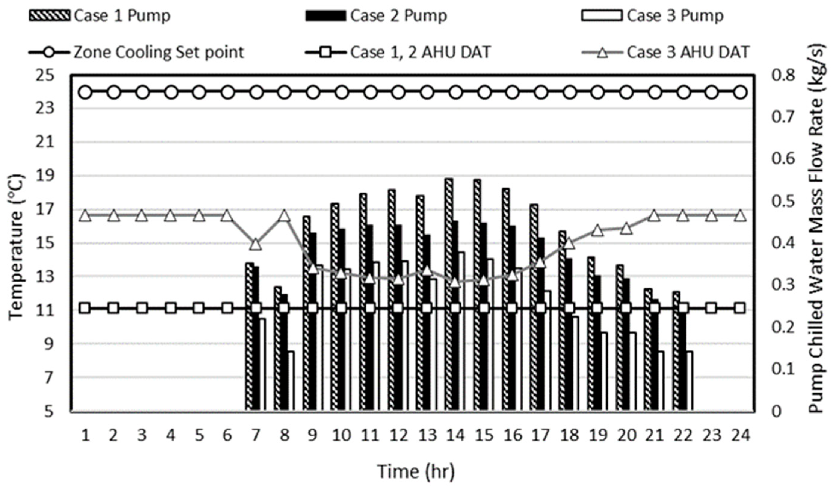
3.2.3. Comparison of the Pump Chilled Water (CHW) Mass Flow Rate on the Summer Representative Day

Figure 14 shows the pump CHW mass flow rate change according to AHU discharge air temperature change on the summer representative day. In Case 1, the average pump CHW mass flow rate was 0.4371 kg/s during the HVAC system operation. In Case 2, the average pump CHW mass flow rate was 0.3785 kg/s. In Case 3, the average pump CHW mass flow rate was 0.2696 kg/s.

Comparing the pump CHW mass flow rate of Case 1 and Case 2, Case 2 required 13.4% less pump CHW mass flow rate. Comparing the pump CHW mass flow rate of Case 1 and Case 3, Case 3 required 38.3% less pump CHW mass flow rate.

The pump CHW mass flow rate is determined by the supply airflow rate and temperature differences between the AHU discharge air temperature and air temperature coming from the mixing box.

The temperature differences between the air temperature from the mixing box and the AHU discharge air temperature increase when the latter is decreased, thus reducing the supply airflow rate but increasing the amount of heat that should be removed from the cooling coil. The pump CHW mass flow rate is increased to remove the increased amount of heat due to high-temperature differences between the air temperature from the mixing box and AHU discharge air temperature. Conversely, temperature differences between air temperature from the mixing box and AHU discharge air temperature decrease, thus increasing the supply airflow rate but decreasing the amount of heat that should be removed from the cooling coil. The pump CHW mass flow rate is decreased to remove the decreased amount of heat due to low-temperature differences between the air temperature from the mixing box and AHU discharge air temperature.

Compared to Cases 1 and 2, as the AHU discharge air temperature in Case 3 increases, the amount of heat that should be removed from the cooling coil decreases. The pump CHW mass flow rate of Case 3 is, therefore, less than that of Cases 1 and 2.

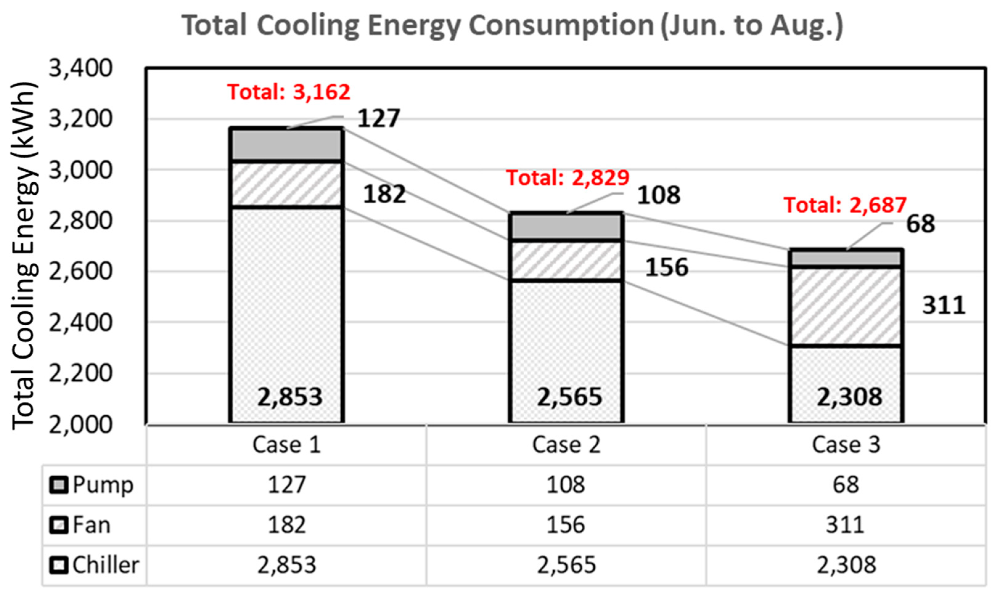
3.2.4. Comparison of the Cooling Energy Consumption on the Summer Representative Day

Table 5. Comparison of the cooling energy consumption in each case on the summer representative day.

	Case 1	Case 2	Case 3
CHW use (kWh/day)	200.26	182.13	172.68
Chiller (COP 5) electric (kWh/day)	40.05	36.43	34.54
Fan electric (kWh/day)	2.65	2.34	3.13
Pump electric (kWh/day)	1.79	1.55	1.10
Total cooling energy (Chiller + Fan + Pump) (kWh/day)	44.49	40.32	38.77

shows the cooling energy consumption in each case on the summer representative day. Cases 1 and 2 consumed CHW about 200.26 kWh/day and 182.13 kWh/day. Case 3 consumed CHW about 172.68 kWh/day on the summer representative day. Comparing the CHW consumption of Case 1 and Case 2, Case 2 consumed 9.1% less CHW. Comparing the CHW of Case 1 and Case 3, Case 3 consumed 13.8% less, and Case 3 consumed 5.2% less CHW when compared with Case 2. Controlling the AHU discharge air temperature through the ANN model showed a significant reduction in CHW consumption compared with fixed AHU discharge air temperature. In all cases, CHW consumption accounted for the large part of the cooling energy.

Table 5 includes the chiller electricity consumption with the assumption of the coefficient of performance (COP) of five for chillers. This COP value is retrieved as a default value from the EnergyPlus program. When all electricity consumptions are combined for chiller, fan, and pump, Case 2 showed 9.4% cooling energy savings and Case 3 12.9% compared to those of Case 1. In the case of fans, Case 3 consumed the largest energy for the reasons described in Section 3.2.3.

3.3. Analysis of Cooling Energy Consumption in the Summer Season

Figure 15 shows the total cooling energy consumption from 1 June to 31 August, which is the summer season, for the three cases. Case 2 consumed about 10.5% less cooling energy than Case 1. In addition, Case 3 consumed about 15.0% less energy than Case 1 and 4.5% less than Case 2. As described above, this paper used the district cooling system; however, we assumed the COP of the chiller as five, and we calculated chiller electric energy consumption to compare the total cooling energy consumption. Fan and pump energy consumption can be interpreted in Section 3.2.2 and Section 3.2.2. The detailed analysis of the cooling energy consumption depending on each case can be interpreted in Figure 16, Figure 17, Figure 18 and Figure 19.

Figure 16, Figure 17 and Figure 18 show the zone mean air temperature and relative humidity of the south zone in each case during the occupied hours, which are between 07:00 to 22:00, from 1 June to 31 August. All cases showed pleasant and appropriate relative humidity values. In Case 1, the indoor air temperature is decreased to 21.9 °C, which is about up to 2.1 °C lower than the thermostat setpoint temperature. In Case 2, the indoor air temperature is decreased to 22.5 °C, which is about up to 1.5 °C lower than the thermostat setpoint temperature. However, in Figure 18, when the ANN-based AHU discharge air temperature control is applied to the building where the DSF system is installed, the indoor air temperature converges at the cooling set temperature, which is 24 °C in the summer season. This is considered to be a result of the fan minimum air flow rate determination method described in Section 3.2.2. Air is continuously supplied to the room, and the amount of supplied air is about 25% of the maximum fan air mass flow rate.

In Cases 1 and 2, the AHU discharge air temperature is fixed at 11.11 °C, and the maximum fan supply air mass flow rate is determined according to the maximum cooling loads. The determined maximum fan supply air mass flow rate affects the minimum fan supply air mass flow rate. Accordingly, even if the cooling loads are low, in Cases 1 and 2, air with a temperature of 11.11 °C is supplied to the zone as the minimum supply fan air mass flow rate. Thus, Figure 16 and Figure 17 are interpreted as the minimum fan air mass flow rate and fixed AHU discharge air temperature.

In Case 3, where indoor air temperature converges to the thermostat setpoint temperature, it can be interpreted in Figure 19. Figure 19 represents cumulative hours and hourly average cooling loads depending on each range of the AHU discharge air temperature in occupied hours in Case 3. The AHU discharge air temperature in Case 3 was divided into six ranges for detailed analysis. As shown in Figure 19, in Case 3, the AHU discharge air temperature is changed depending on the cooling loads. Therefore, in Case 3, when the required cooling loads are low, the AHU discharge air temperature is increased. This is why overcooling does not occur in Case 3, unlike Cases 1 and 2.

4. Conclusions

The goal of this study was to verify potential cooling energy savings by applying ANN-based control of AHU discharge air temperature in DSF office buildings in a hot and humid climate. The ANN model predicted cooling loads within the CVRMSE value of 4.6% after the optimization process, which is within the tolerance range of 30% recommended by the ASHRAE Guideline 14. It was observed that a considerable amount of cooling energy could be saved from using ANN-based control compared to the simple fixed control method. Results showed that 10.5% of cooling energy savings can be achieved with the installation of the DSF itself to a non-DSF building. Additional cooling energy savings of 4.5% can be realized by applying an ANN-based AHU discharge air temperature control method to the DSF building. This study observed that overcooling occurred with the conventional HVAC control method due to the minimum fan air mass flow rate and the fixed AHU discharge air temperature. By the application of ANN-based AHU discharge air temperature control methods, the indoor air temperature is constantly maintained to the thermostat set temperature of 24.0 °C with minimal variations. Cooling energy savings were obtained from the removal of overcooling hours, which were possible from the optimal control of discharge air temperature using the ANN-based control algorithms. This paper presented energy savings results for the cooling season only. Because the air temperature inside the DSF system is higher than the outdoor air temperature, heating energy can also be saved in winter. In the future, annual energy savings analyses will be conducted, including cooling, heating, and swing seasons altogether by applying advanced ANN-based control algorithms. Also, this paper focused only on one floor in a multi-story building; however, a whole building energy analysis will be conducted in the future.

References

1. Lee, D.Y.; Seo, B.M.; Yoon, Y.B.; Hong, S.H.; Choi, J.M.; Lee, K.H. Heating energy performance and part load ratio characteristics of boiler staging in an office building. Front. Energy 2019, 13, 339–353. [Google Scholar] [CrossRef]
2. U.S. Energy Information Administration (EIA)/Annual Energy Outlook. 2019. Available online: https://www.eia.gov/outlooks/aeo/ (accessed on 18 November 2019).
3. Ghaffarianhoseini, A.; Ghaffarianhoseini, A.; Berardi, U.; Tookey, J.; Li, D.H.W.; Kariminia, S. Exploring the advantages and challenges of double-skin facades (DSFs). Renew. Sustain. Energy Rev. 2016, 60, 1052–1065. [Google Scholar] [CrossRef]
4. Yoon, Y.B.; Seo, B.; Koh, B.B.; Cho, S. Performance analysis of a double-skin facade system installed at different floor levels of high-rise apartment building. J. Build. Eng. 2019, 26, 100900. [Google Scholar] [CrossRef]
5. Joe, J.; Choi, W.; Kwak, Y.; Huh, J.H. Optimal design of a multi-story double skin facade. Energy Build. 2014, 76, 143–150. [Google Scholar] [CrossRef]
6. Kim, D.; Cox, S.J.; Cho, H.; Yoon, J. Comparative investigation on building energy performance of double skin facade (DSF) with interior or exterior slat blinds. J. Build. Eng. 2018, 20, 411–423. [Google Scholar] [CrossRef]
7. Shameri, M.A.; Alghoul, M.A.; Sopian, K.; Zain, M.F.M.; Elateb, O. Perspectives of double skin facade systems in buildings and energy saving. Renew. Sustain. Energy Rev. 2011, 15, 1468–1475. [Google Scholar] [CrossRef]
8. Raji, B.; Tenpierik, M.J.; Dobbelsteen, A. An assessment of energy-saving solutions for the envelope design of high-rise buildings in temperate climates: A case study in the Netherlands. Energy Build. 2016, 124, 210–221. [Google Scholar] [CrossRef]
9. Joe, J.; Choi, W.; Kwon, H.; Huh, J.H. Load characteristics and operation strategies of building integrated with multi-story double skin facade. Energy Build. 2013, 60, 185–198. [Google Scholar] [CrossRef]
10. Choi, W.; Joe, J.; Kwak, Y.; Huh, J.H. Operation and control strategies for multi-storey double skin facades during the heating season. Energy Build. 2017, 49, 454–465. [Google Scholar] [CrossRef]
11. Chan, A.L.S.; Chow, T.T.; Fong, K.F.; Lin, Z. Investigation on energy performance of double skin facade in Hong Kong. Energy Build. 2009, 41, 1135–1142. [Google Scholar] [CrossRef]
12. Hamza, N. Double versus single skin facades in hot arid areas. Energy Build. 2008, 40, 240–248. [Google Scholar] [CrossRef]
13. Souza, L.C.O.; Souza, H.A.; Rodrigues, E.F. Experimental and numerical analysis of a naturally ventilated double skin façade. Energy Build. 2018, 165, 328–339. [Google Scholar] [CrossRef]
14. Zomorodian, Z.S.; Tahsildoost, M. Energy and carbon analysis of double skin façades in the hot and dry climate. J. Clean. Prod. 2018, 197, 85–96. [Google Scholar] [CrossRef]
15. Gratia, E.; Herde, A.D. Are energy consumptions decreased with the addition of a double-skin? Energy Build. 2007, 39, 605–619. [Google Scholar] [CrossRef]
16. Gelesz, A.; Reith, A. Climate-based performance evaluation of double skin façade by building energy modelling in Central Europe. In Proceedings of the 6th International Building Physics Conference (IBPC2015), Torino, Italy, 14–17 June 2015. [Google Scholar]
17. Moon, J.W.; Lee, J.H.; Kim, S. Application of control logic for optimum indoor thermal environment in buildings with double skin envelope systems. Energy Build. 2014, 85, 59–71. [Google Scholar] [CrossRef]
18. Moon, J.W.; Lee, J.H.; Yoon, Y.; Kim, S. Determining optimum control of double skin envelope for indoor thermal environment based on artificial neural network. Energy Build. 2014, 69, 175–183. [Google Scholar] [CrossRef]
19. Moon, J.W.; Yoon, S.H.; Kim, S. Development of an artificial neural network model based thermal control logic for double skin envelopes in winter. Build. Environ. 2013, 61, 149–159. [Google Scholar] [CrossRef]
20. Moon, J.W.; Part, J.C.; Kim, S. Development of control algorithms for optimal thermal environment of double skin envelope buildings in summer. Build. Environ. 2018, 144, 657–672. [Google Scholar] [CrossRef]
21. Moon, J.W. Integrated control of the cooling system and surface openings using the artificial neural networks. Appl. Therm. Eng. 2015, 78, 150–161. [Google Scholar] [CrossRef]
22. Moon, J.W.; Lee, J.H.; Chang, J.D.; Kim, S. Preliminary performance tests on artificial neural network models for opening strategies of double skin envelopes in winter. Energy Build. 2014, 75, 301–311. [Google Scholar] [CrossRef]
23. Alberto, A.; Ramos, N.M.M.; Almeida, R.M.S.F. Parametric study of double-skin facades performance in mild climate countries. J. Build. Eng. 2017, 12, 87–98. [Google Scholar] [CrossRef]
24. Lee, J.M.; Seo, B.M.; Hong, S.H.; Lee, K.H. Application of Artificial Neural Networks for Optimized AHU Discharge Air Temperature Set-point and Minimized Cooling Energy in VAV System. Appl. Therm. Eng. 2019, 153, 726–738. [Google Scholar] [CrossRef]
25. Yeon, S.H.; Yu, B.; Seo, B.M.; Yoon, Y.B.; Lee, K.H. ANN Based Automatic Slat Angle Control of Venetian Blind for Minimized Total Load in an Office Building. Sol. Energy 2019, 180, 133–145. [Google Scholar] [CrossRef]
26. Seo, B.; Yoon, Y.B.; Song, S.; Cho, S. ANN-based thermal load prediction approach for advanced controls in building energy systems. In Proceedings of the Conference for ARCC 2019 International Conference, Toronto, ON, Canada, 29 May–1 June 2019. [Google Scholar]
27. The U.S. DOE. Getting Started. EnergyPlus Version 9.1.0 Documentation; The U.S. DOE: Washington, DC, USA, 2019.
28. The U.S. DOE. EnergyPlus Engineering Reference. The Reference to EnergyPlus Calculations, Version 9.1; The U.S. DOE: Washington, DC, USA, 2019.
29. Seo, B.M.; Lee, K.H. Detailed analysis on part load ratio characteristics and cooling energy saving of chiller staging in an office building. Energy Build. 2016, 119, 309–322. [Google Scholar] [CrossRef]
30. Lutz, M.; Ascher, D. Learning Python, 5th ed.; O’Reilly: Sebastopol, CA, USA, 2013. [Google Scholar]
31. The U.S. DOE. EnergyPlus Input Output Reference: The Encyclopedic Reference to EnergyPlus Input and Output, Version 9.1; The U.S. DOE: Washington, DC, USA, 2019.
32. American Society of Heating, Refrigerating and Air-Conditioning Engineers (ASHRAE). Handbook of Fundamentals; American Society of Heating, Refrigerating and Air-Conditioning Engineers Inc.: Atlanta, GA, USA, 2009; Volume 30329(404). [Google Scholar]
33. Costola, D.; Etheridge, D.W. Unsteady natural ventilation at model scale-Flow reversal and discharge coefficients of a short stack and an orifice. Build. Environ. 2008, 43, 1491–1506. [Google Scholar] [CrossRef]
34. Schulze, T.; Eicker, U. Controlled natural ventilation for energy efficient buildings. Energy Build. 2013, 56, 221–232. [Google Scholar] [CrossRef]
35. Rashid, T. Make Your Own Neural Network. CreateSpace Independent Publishing Platform, 2016 Hargan, MR., ASHRAE Guideline 14-2002 Measurement of Energy and Demand Savings; American Society of Heating Refrigerating and Air-Conditioning Engineers Inc.: Atlanta, GA, USA, 2012. [Google Scholar]
Figure 1. Simulation model.
Energies 12 04754 g001
Figure 2. Internal heat gain and HVAC system schedules for weekdays.
Energies 12 04754 g002
Figure 3. System diagram.
Energies 12 04754 g003
Figure 4. Processes in the predictive ANN model.
Energies 12 04754 g004
Figure 5. Initial ANN structure.
Energies 12 04754 g005
Figure 6. Structure of the python programming code for the optimization process.
Energies 12 04754 g006
Figure 7. Optimal ANN structure.
Energies 12 04754 g007
Figure 8. Comparison of simulation data and ANN results.
Energies 12 04754 g008
Figure 9. Outdoor air dry-bulb temperature and relative humidity in Miami, Florida.
Energies 12 04754 g009
Figure 10. Comparison of the cooling loads and the AHU discharge air temperatures in each case on the summer representative day.
Energies 12 04754 g010
Figure 11. Window heat gain rate in the zone through the south exterior window.
Energies 12 04754 g011
Figure 12. Comparison of inside air temperature with the installation of the DSF system.
Energies 12 04754 g012
Figure 13. Comparison of fan mass flow rate according to AHU discharge air temperature change.
Energies 12 04754 g013
Figure 14. Comparison of pump CHW mass flow rate according to AHU discharge air temperature change.
Energies 12 04754 g014
Figure 15. Comparison of the total cooling energy consumption.
Energies 12 04754 g015
Figure 16. Indoor air temperature and relative humidity of Case 1 in the summer season.
Energies 12 04754 g016
Figure 17. Indoor air temperature and relative humidity of Case 2 in the summer season.
Energies 12 04754 g017
Figure 18. Indoor air temperature and relative humidity of Case 3 in the summer season.
Energies 12 04754 g018
Figure 19. Cumulative operation hours and hourly average cooling load in each AHU discharge air temperature range.
Energies 12 04754 g019