A Control-Oriented Engine Torque Online Estimation Approach for Gasoline Engines Based on In-Cycle Crankshaft Speed Dynamics

Abstract

Engine brake torque is a key feedback variable for the optimal torque split control of an engine–motor hybrid powertrain system. Due to the limitations in available sensors, however, engine torque is difficult to measure directly. For torque estimation, the unknown external load torque and the overlap of the expansion stroke between cylinders introduce a great disturbance to engine speed dynamics. This makes the conventional cycle average engine speed-based estimation approach unusable. In this article, an in-cycle crankshaft speed-based indicated torque estimation approach is proposed for a four-cylinder engine. First, a unique crankshaft angle window is selected for load torque estimation without the influence of combustion torque. Then, an in-cycle angle-domain crankshaft speed dynamic model is developed for engine indicated torque estimation. To account for the effects of model inaccuracy and unknown external disturbances, a “total disturbance” term is introduced. The total disturbance is then estimated by an adaptive observer using the engine’s historical operating data. Finally, a real-time correction method for the friction torque is proposed in the fuel cut-off scenario. Combining the aforementioned torque estimators, the brake torque can be obtained. The proposed algorithm is implemented in an in-house developed multi-core engine control unit (ECU). Experimental validation results on an engine test bench show that the algorithm’s execution time is about 3.2 ms, and the estimation error of the brake torque is within 5%. Therefore, the proposed method is a promising way to accurately estimate engine torque in real-time.

1. Introduction

Engine–motor hybrid powertrain systems have been widely used in passenger vehicles [1] to meet increasingly strict emission legislation and improve fuel economy. Optimal torque split between the engine and torque is obviously essential to achieve the best overall efficiency for hybrid vehicles.

Due to the fundamental nature of internal combustion engines (ICEs), the torque’s response is slower than the motor’s and is usually difficult to measure directly [2,3]. The degradation in engine torque control performance will, in turn, have an adverse effect on the overall fuel economy of the hybrid powertrain systems [4]. This drives the need for real-time estimation of the engine torque, especially in the application of hybrid electric vehicles (HEVs) [5].

Various solutions were available for engine torque control in the past. The most straightforward method to measure the engine torque is by in-cylinder pressure sensors or torque sensors. These solutions, however, increase the hardware cost and create an issue of durability. For instance, the cylinder’s pressure may suffer from its harsh thermal environment. These factors limit the application of this method in stock engines [6,7,8,9].

An alternative cost-effective solution without the need for additional sensors is to use a crankshaft instantaneous speed sensor, based on the causality between the engine torque and engine speed variation [10,11]. Theoretically, any changes in the engine brake torque can be sensed from the fluctuation of the crankshaft’s instantaneous speed [12]. Three methodologies are commonly used in crankshaft speed-based torque estimation, consisting of black-box model-based estimation, frequency analysis-based mapping, and crankshaft dynamic model-based estimation [13]. The first solution is to use a black-box model (such as a neural network and nominal function) to describe the relationship between the engine torque and crankshaft instantaneous speed [14,15,16,17,18]. However, these methods need an amount of data to train the black-box model. Moreover, their model parameters vary with the operating conditions caused by the nonlinear nature of the engine speed dynamics. This makes a single model unsuitable for estimating engine torque under all operating conditions. To improve the estimation accuracy, a piece-wise linear model is a popular solution but comes at the cost of a heavy workload during calibration.

Frequency analysis-based mapping [19] can be used to estimate the indicated torque. After the crankshaft’s instantaneous speed and indicated torque are processed by DFT (discrete Fourier transform), a significantly positive correlation can be observed between the two signals in the main harmonic order [20]. However, this requires complicated signal and computational processing and is unsuitable for online applications in the engine control unit (ECU). The third approach is to use crankshaft dynamic models, which can be expressed in the torque balance equation [21,22,23,24,25]. The crankshaft dynamics model can be divided into two categories: A rigid model and an elastic model [26]. The elastic crankshaft dynamics model has higher prediction accuracy and wider working conditions than the rigid model. However, the elastic model requires a large amount of calculation work, which limits its use in real-time applications [13].

In order to increase the adaptability and accuracy of the torque estimation algorithm, the intake process and combustion process are also considered in crankshaft speed modeling. Obviously, this makes the physical model too complicated to implement in an ECU without many model parameters for calibration [27]. Additionally, for the engine friction torque estimation, a look-up table approach is simple to implement and shows degraded estimation accuracy with the aging of the engine [28]. In addition, the unknown resistance torque from the gear box and the wheel makes the engine speed-based engine torque estimation more challenging. To sum up, it is clear that the on-board torque estimation algorithm is challenging, due to the dilemma between the estimation’s accuracy and its feasibility in embedded system implementation [13].

Currently, the existing torque online estimation methods are primarily based on look-up tables calibrated offline. This is simple-to-straightforward to implement, but the estimation accuracy deteriorates as the engine ages. One contribution of the proposed algorithm is the ability to be adaptive to the aging of the engine.

In this paper, an engine brake torque estimation approach is proposed for a four-cylinder engine, consisting of the load torque estimator, indicated torque estimator, and a friction torque observer. In fact, the brake torque estimation is valid for both four-cylinder and three-cylinder engines. For engines with a cylinder number equal or less than four, there exists a unique crankshaft angle window, where there is no overlap of the combustion processes. For engines with more than four cylinders, such kind of crankshaft window does not exist, which affects the estimation of total gas torque. First, the load torque estimator is designed for the unique crankshaft angle window. Then, an in-cycle angle-domain crankshaft speed dynamic model is developed for engine-indicated torque estimation with a deviation from the model of a real plant lumped as the total disturbance for estimation. Finally, a real-time correction method for the friction torque is proposed for use in a fuel cut-off scenario. The proposed algorithm is implemented in a multicore ECU to testify its accuracy, computational time, and central processing unit (CPU) loads.

The rest of this article is organized as follows. In Section 2, the experiment setup is discussed briefly. Then, an engine torque observer algorithm is proposed in Section 3. The engine torque observer estimation results and embedded performance are discussed in Section 4. Finally, the conclusions of this study are shown in Section 5.

2. Experiment Setup

The experiment was conducted on a Greatwall Motor EC02 GDI (Gasoline Direct Injection) engine test bench (as shown in Figure 1) with a Horiba DYNAS3 LI 250 electric dynamometer. The schematic diagram of the test bench is shown in Figure 2. The engine has a firing order of 1-3-4-2, and all four cylinders are equipped with in-cylinder pressure sensors for the indicated torque estimation (the baseline for observer validation). The detailed engine specifications are tabulated in

Table 1. Engine specifications.

Variable	Value
Displacement (liter)	2.0 L
Cylinders	4
Compression ratio	9.6
Bore (mm)	82.5
Stroke (mm)	92
Connecting rod (mm)	144
Maximum torque (Nm)/speed (rpm)	385/1800
Rated power (kW)/speed (rpm)	165/5500
Intake mode	Naturally aspired

.

3. Engine Torque Observer Development

In this section, the derivation of the proposed engine torque estimation algorithm is discussed in detail, including engine dynamic model identification, the indicated torque observer [29], and the brake torque observer.

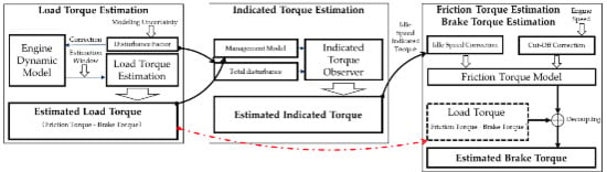
3.1. Engine Dynamic Model

The instantaneous rotational speed of the crankshaft is affected by the torque enforced by the crankshaft following Newton’s law. In the crankshaft dynamics, a combination of the brake torque, the friction torque, the indicated torque, and the reciprocating inertia torque works on the crankshaft, causing engine instantaneous speed to fluctuate. There are two kinds of dynamic model in literature, the elastic model and the rigid-body model. The rigid-body model is simplified from the elastic model. Although the elastic model of the crankshaft has high accuracy, the calculation process needs to consume more computing resources. The rigid-body crankshaft dynamic model needs less computing resources, but it has a lower accuracy. This section proposes a rigid-body crankshaft model with a disturbance factor (1), which is used to compensate the error caused by dynamic model simplification process.

$$\left[J+\Delta \xi \left(\theta \right)\right]\ddot{\theta }=T_{ind}-T_r-T_{fric}-T_e$$

(1)

where $J$ is the rotational inertia of the crankshaft, $\theta$ is the rotation angle of the crankshaft, $\Delta \xi \left(\theta \right)$ is the disturbance factor, $\ddot{\theta }$ is the angular acceleration of the crankshaft, $T_{ind}$ is the indicated torque, $T_r$ is the reciprocating inertia torque, $T_{fric}$ is the friction torque, and $T_e$ is the brake torque.

As seen in Equation (1), the angular acceleration is the second-order derivative of the crankshaft rotation angle ($\ddot{\theta }$), which is very noisy. So, a finite impulse response (FIR) filter is used to process the angular speed signal with a cut-off frequency of 300 Hz. A Kalman filter is used to calculate the angular acceleration.

3.1.1. Reciprocating Torque

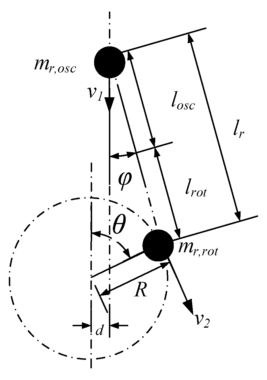
The reciprocating torque is generated by the reciprocating part of the connecting rod system. The schematic diagram of the movement of the connecting rod system is as follows in Figure 3.

$m_{r,osc}$ is the reciprocating mass of the system, including the piston group and the reciprocating part of the connecting rod. $l_{osc}$ is the length of the reciprocating part of crank connecting rod mechanism. $m_{r,rot}$ is the rotation mass of the system, including the crankshaft and the rotation part of the connecting rod mechanism, and $l_{rot}$ is the length of the rotating part of the connecting rod. $l_r$ denotes the length of the connecting rod. $R$ is radius of the crank. $\theta$ is the crankshaft rotation angle. $\phi$ denotes the connecting rod angle. ${\nu }_1$ is the velocity of the piston. ${\nu }_2$ is the linear velocity of the crank. $d$ denotes the piston pin offset, which is neglected in this research.

According to the law of conservation of energy, the system’s kinetic energy consists of the kinetic energy of the reciprocating mass and the rotation mass, which can be expressed as Equation (2) [23].

$$J{\dot{\theta }}^2=m_{r,osc}{\nu }_1{}^2+m_{r,rot}{\nu }_2{}^2$$

(2)

The velocities of the reciprocating mass and the rotation mass can be expressed as:

$$\{\begin{array}{l}{\nu }_1=R\dot{\theta }[sin\theta +\frac{{\lambda }_{r}sin2\theta }{2\sqrt{1-{\lambda }_r{}^{2}si{n}^2\theta }}]\hfill \\ {\nu }_2=R\dot{\theta }\hfill \end{array}$$

(3)

where ${\lambda }_r=\left(R/l_r\right)$ denotes the crank radius to connecting rod length ratio [23].

So, according to Equations (2) and (3), the moment of inertia of the system can be expressed as:

$$J=m_{r,osc}{R}^2[sin\theta +\frac{{\lambda }_{r}sin2\theta }{2\sqrt{1-{\lambda }_r{}^{2}si{n}^2\theta }}]+m_{r,rot}{R}^2$$

(4)

$T_r$ denotes the reciprocating torque [23].

$$T_r=m_{r,osc}{R}^{2}f\left(\theta \right)\left[f\left(\theta \right)\ddot{\theta }+g\left(\theta \right){\dot{\theta }}^2\right]$$

(5)

where:

$$f\left(\theta \right)=sin\theta +\frac{{\lambda }_{r}sin2\theta }{2\sqrt{1-{\lambda }_r{}^{2}si{n}^2\theta }}$$

$$g\left(\theta \right)=cos\theta +\frac{{\lambda }_{r}sin2\theta }{\sqrt{1-{\lambda }_r{}^{2}si{n}^2\theta }}+\frac{{\lambda }_r{}^{3}si{n}^2\left(2\theta \right)}{4\sqrt{1-{\lambda }_r{}^{2}si{n}^2\theta }}.$$

The total reciprocating torque can be written as:

$$T_r={\displaystyle {\displaystyle \sum }_{k=1}^N}{T}_r^{\left(k\right)}=m_{r,osc}{R}^2{\displaystyle {\displaystyle \sum }_{k=1}^N}f\left(\theta -{\varphi }_k\right)[f\left(\theta -{\varphi }_k\right)\ddot{\theta }+g\left(\theta -{\varphi }_k\right){\dot{\theta }}^2]$$

(6)

where:

$${\varphi }_k=\frac{4\pi }{N}\left(k-1\right).$$

$N$ is the number of cylinders, in this case $N=4$. ${\varphi }_k$ ($k=1,\dots ,N$) denotes the phase of the $k$th cylinder [13].

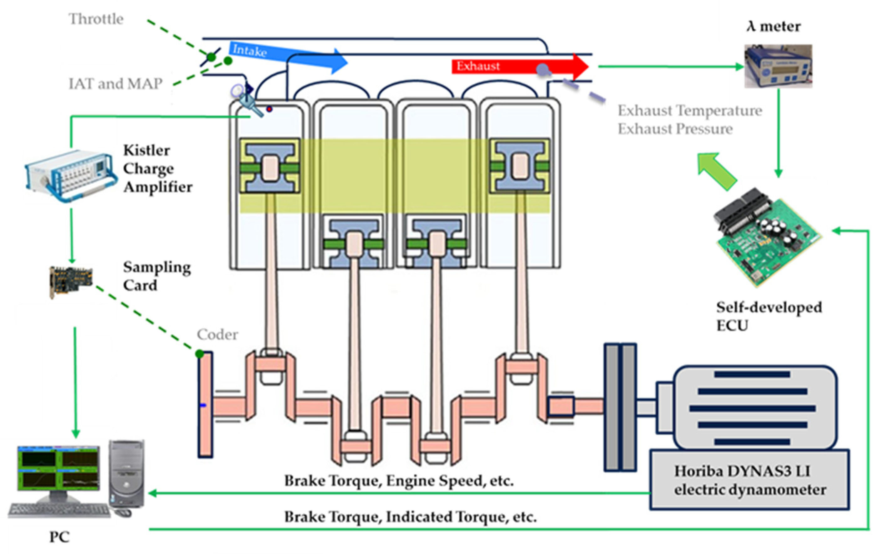
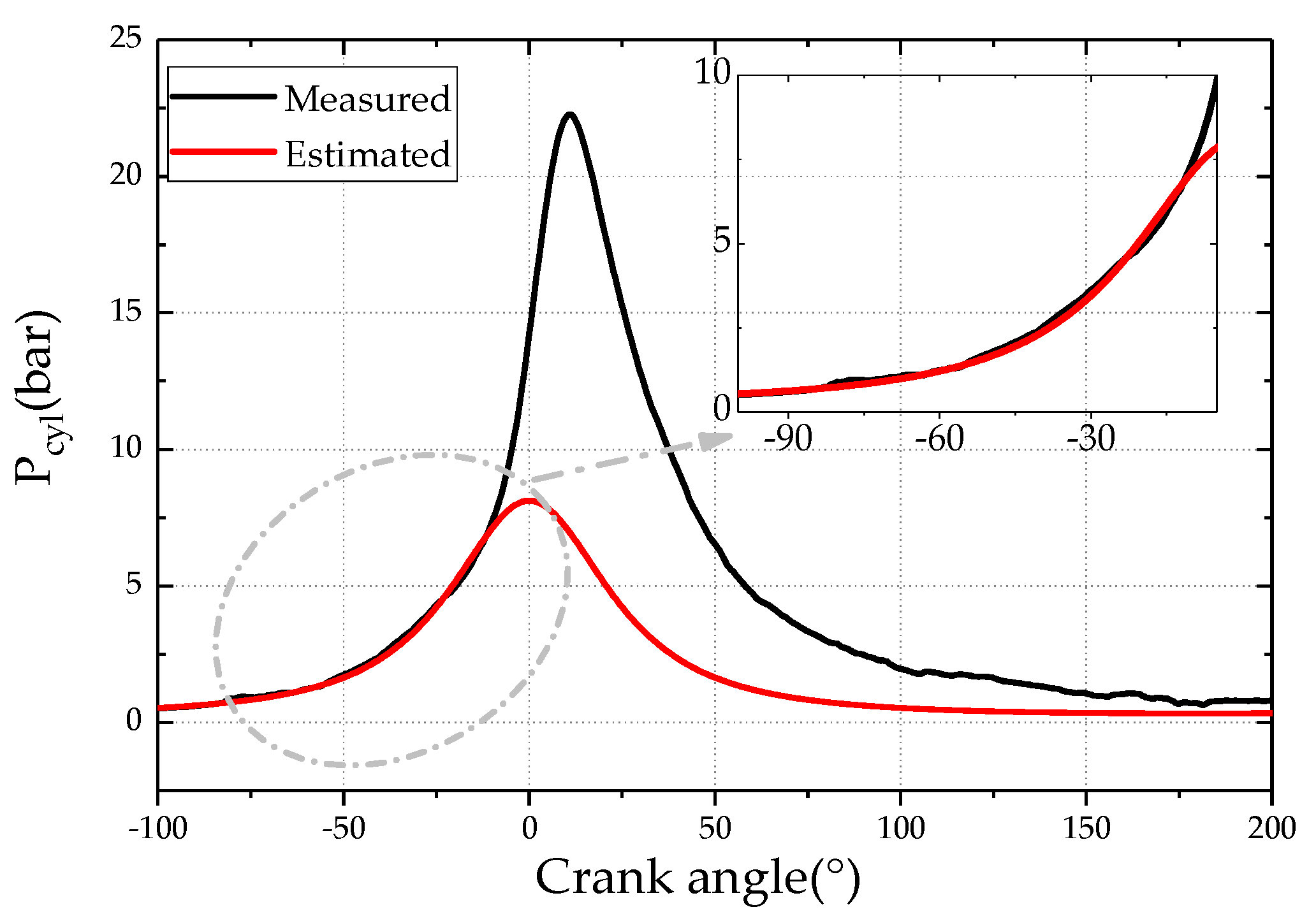
3.1.2. Indicated Torque Estimation

Indicated torque is generated at two process, the compression process and the combustion process. The indicated torque during combustion process is difficult to estimate. However, the compression process can be considered as a polytropic process, the in-cylinder pressure can be estimated using the manifold absolute pressure (MAP) sensor and the intake air temperature (IAT) sensor, assuming that the in-cylinder pressure can be approximated by MAP at the timing of intake valve closing and corrected by volumetric efficiency. The MAP sensor and IAT sensor are already standard sensors equipped in stock engines. The estimated pressure then can be used to calculate the indicated torque during compression process, shown in Figure 4.

$$P_{cyl}{V}^{\kappa }=const$$

(7)

where $P_{cyl}$ denotes the in-cylinder pressure; $V$ denotes the gas volume; and $\kappa$ is the polytropic process factor, which is taken to be 1.3 in this research within the compression stoke [21].

$$V=V_c+(R+l_r-Rcos\theta -l_r\sqrt{1-{\lambda }_r{}^{2}si{n}^2\theta })\frac{\pi B^2}{4}.$$

(8)

where $V_c$ is the combustion chamber volume, and $B$ is the cylinder diameter [22].

The total indicated torque is:

$$T_{ind}={{\displaystyle \sum }}_{k=1}^N{T}_{ind}^{\left(k\right)}=\frac{\pi B^2}{4}R{{\displaystyle \sum }}_{k=1}^N[P_{cyl}{}^{\left(k\right)}f\left(\theta -{\varphi }_k\right)].$$

(9)

3.1.3. Load Torque Estimation

For an internal combustion engine, the load torque ($T_{load}$) involves two parts: The brake torque ($T_e$) and the friction torque ($T_{fric}$). $T_{load}$ a slow-varying variable compared to the combustion process, so $T_{load}$ can be considered approximately as a constant in one cycle. In the crankshaft dynamic model, both $T_{load}$ and $T_{ind}$ are unknown variables, which makes $T_{load}$ difficult to estimate. In Section 3.1.2, $T_{ind}$ during the compression process can be estimated, which can be defined as gas torque ($T_{gas}$). For four-cylinder engines and engines with less than four cylinders, there is a unique crankshaft angle window, where the sum of the other three cylinders can be neglected [21]. Within this particular crankshaft angle window, the total indicated torque can be calculated from the cylinder in the compression phase. A $T_{load}$ estimator can be designed in this window, where there is no combustion, even for all cylinders. A bench test was done to locate this angle window, and experimental result shows that 50 crank angle before TDC to 20 crank angle before TDC is the unique angle window to estimate the total gas torque for all cylinders. Meanwhile, this angle window can be used to estimate $T_{load}$ and $\Delta \xi \left(\theta \right)$.

In the unique crankshaft angle window from 50° before TDC to 20° before TDC, the only unknown variables are $T_{load}$ and $\Delta \xi \left(\theta \right)$. So the $T_{load}$ estimation issue can be regarded as a system parameter estimation issue. The least-squares method is a method for identifying system parameters. However, there are few sampling points in the unique window, and the least-squares method is challenging for online applications. So $T_{load}$ estimation algorithm using the recursive least-squares method is proposed, and the algorithm can process the sampling data in multiple cycles. The estimated load torque (${\widehat{T}}_{load}$) at the end of last cycle will be set as the initial load torque into the engine load torque estimator. ${\widehat{T}}_{load}$ and $\Delta \xi \left(\theta \right)$ are key variables for $T_{ind}$ observer in the next section.

The specific algorithm is shown in Figure 5. The manifold absolute pressure at intake valve close (IVC) $P_{MAP\_IVC}$ is used to calculate $T_{gas}$.

During the unique crankshaft angle window, Equation (1) can be transformed as:

$$T_u=J_e\ddot{\theta }+T_{load}.$$

(10)

where:

$$T_{load}=T_{fric}+T_e,T_u=T_{gas}-T_r,J_e=J+\Delta \xi \left(\theta \right)$$

For the K times of successive sampling, Equation (10) can be:

$$\left[\begin{array}{c}{T}_u\left(1\right)\\ ⋮\\ T_u\left(K\right)\end{array}\right]=\left[\begin{array}{cc}\ddot{\theta }\left(1\right)& 1\\ ⋮& ⋮\\ \ddot{\theta }\left(K\right)& 1\end{array}\right]\left[\begin{array}{c}{J}_e\\ T_{load}\end{array}\right]+\left[\begin{array}{c}\varsigma \left(1\right)\\ ⋮\\ \varsigma \left(K\right)\end{array}\right].$$

(11)

where $\varsigma$ is white noise with mean value 0.

So Equation (11) can be described as:

$${\mathit{T}}_K={\Phi }_K{\Theta }_K+{\mathit{\varsigma }}_K$$

(12)

$${\mathit{T}}_K=\left[\begin{array}{c}{T}_u\left(1\right)\\ ⋮\\ T_u\left(K\right)\end{array}\right],{\Phi }_K=\left[\begin{array}{cc}\ddot{\theta }\left(1\right)& 1\\ ⋮& ⋮\\ \ddot{\theta }\left(K\right)& 1\end{array}\right],{\Theta }_K=\left[\begin{array}{c}{J}_e{}_K\\ T_{load}{}_K\end{array}\right],{\mathit{\varsigma }}_K=\left[\begin{array}{c}\varsigma \left(1\right)\\ ⋮\\ \varsigma \left(K\right)\end{array}\right]$$

According to the recursive least-squares method:

$${\widehat{\Theta }}_K={\mathit{P}}_K{\Phi }_K{}^T{\mathit{T}}_K$$

(13)

$${\mathit{P}}_K={\left({\Phi }_K{}^T{\Phi }_K\right)}^{-1}$$

For $K$+1, when a new $\ddot{\theta }\left(K+1\right)$ and $T_u\left(K+1\right)$ are calculated, we define ${\mathit{\Psi }}_{K+1}=[\begin{array}{cc}\ddot{\theta }\left(K+1\right)& 1\end{array}]$, so:

$${\mathit{P}}_{K+1}={\left({\mathit{P}}_K{}^{-1}+{\mathit{\Psi }}_{K+1}{\mathit{\Psi }}_{K+1}{}^T\right)}^{-1}.$$

(14)

Then the $\widehat{\mathit{\Theta }}$ can be estimated using recursive least-squares method:

$$\{\begin{array}{l}{\mathit{Q}}_{K+1}={\mathit{P}}_K{\mathit{\Psi }}_{K+1}{\left(1+{\mathit{\Psi }}_{K+1}{}^T{\mathit{P}}_K{\mathit{\Psi }}_{K+1}\right)}^{-1}\hfill \\ {\mathit{P}}_{K+1}={\mathit{P}}_K-{\mathit{Q}}_{K+1}{\mathit{\Psi }}_K{}^T{\mathit{P}}_K\hfill \\ {\widehat{\mathit{\Theta }}}_{K+1}={\widehat{\mathit{\Theta }}}_K+{\mathit{Q}}_{K+1}({\mathit{T}}_{K+1}-{\mathit{\Psi }}_{K+1}{}^T{\widehat{\mathit{\Theta }}}_K)\hfill \end{array}$$

(15)

The convergence of $\widehat{\mathit{\Theta }}$ requires a certain amount of $T_u$ and $\ddot{\theta }$. Therefore, the recursive process is expanded to multiple cycles, that is, the initial value of the estimated parameter $\widehat{\mathit{\Theta }}$, including $T_{load}$ and $\Delta \xi \left(\theta \right)$, is the result of the last estimated value from the previous cycle.

3.2. Indicated Torque Observer

3.2.1. Engine Management Model

This engine management model is a serious model to calculate the initial indicated torque $T_{indini}$, and the model is the base of the extended state observer (ESO) to estimate the indicated torque. The engine management model contains the thermal efficiency model, the crankshaft dynamic model, etc. [30].

The indicated work comes from the combustion process of the delivered fuel, and can be modeled as a function of fuel heating value, the delivered mass of the gasoline and the operation conditions [30]. The indicated work can be expressed as:

$$W_{ind}=m_f{q}_{LHV}{E}_{ff}$$

(16)

where $W_{ind}$ is indicated work, $m_f$ is the delivered gasoline mass, $q_{LHV}$ is gasoline heating value. $E_{ff}$ is thermal efficiency, which can be expressed as:

$$E_{ff}=\left(1-\frac{1}{r_c^{\kappa -1}}\right)·\min \left(1,\lambda \right)·{\eta }_{ign}\left({\theta }_{ign}\right)·{\eta }_{ig,ch}(\dot{\theta },V_d)$$

(17)

where $r_c$ denotes the compression ratio, $V_d$ is the engine displacement, ${\theta }_{ign}$ is the position for the ignition timing, ${\eta }_{ign}$ is the ignition efficiency, ${\eta }_{ig,ch}(\dot{\theta },V_d)$ is the heat transfer efficiency between the real and the ideal cycles, $\lambda$ denotes the air/fuel ratio, and $\min \left(1,\lambda \right)$ describes that the fuel mass cannot fully utilized in the case of a rich mixture [30].

The engine dynamic model used in this section is already mentioned in Section 3.1

3.2.2. Indicated Torque Observer Design

Here, an indicate torque observation method is built using ESO. The indicated thermal efficiency $E_{ff}$ is the key parameter to calculate the indicated torque. However, the $E_{ff}$ is a state parameter of the combustion process, which is impossible to measure. So an ESO is built on the base of the engine management model, the uncertainty of the indicated thermal efficiency $\Delta E_{ff}$ is proposed to compensate the total error of the engine management model. The indicated torque observer based on ESO is shown in Figure 6.

The intake air quantity ($Q_{mass}$) used to calculate the initial indicated torque, along with the $T_{load}$ estimated in Section 3.1.3, are processed by crankshaft dynamic model into engine rotation speed $\dot{\theta }$. The engine speed simulated by the crankshaft dynamic model is compared with the engine speed measured. The error between the simulated engine speed and the measured engine speed is obtained by ESO-based indicated thermal efficiency observer to calculate the $\Delta E_{ff}$. Once the $\Delta E_{ff}$ is calculated, the indicated torque ${\widehat{T}}_{ind}$ can be calculated using $\Delta E_{ff}$, $Q_{mass},$ and $\lambda .$ The detailed solution consists of system modeling in Equation (18), the model-based ESO design as Equation (20), and the ESO parameter tuning as Equation (23).

The crankshaft dynamic model can be described as a first order linear system, as in Equation (18):

$$\ddot{\theta }=\frac{4\phi }{4\pi \lambda \left[J+\Delta \xi \left(\theta \right)\right]}\left(E_{ff}+\Delta E_{ff}\right)Q_{mass}-\frac{1}{J+\Delta \xi \left(\theta \right)}{T}_{fric}-\frac{1}{J+\Delta \xi \left(\theta \right)}{T}_e.$$

(18)

The ESO can be described as:

$$\{\begin{array}{l}\dot{z}=\mathit{A}x+\mathit{B}u+\mathit{L}\left(y-\widehat{y}\right)\hfill \\ \widehat{y}=\mathit{C}z\hfill \end{array}$$

(19)

where $z$ is the estimated value of $x$, and $\widehat{y}$ is the estimated value of $y$ [31]. So, Equation (18) can be described as:

$$\{\begin{array}{l}{\dot{z}}_1=a_1\left(E_{ff}+z_2\right)Q_{mass}-\frac{1}{J+\Delta \xi \left(\theta \right)}{T}_{fric}-\frac{1}{J+\Delta \xi \left(\theta \right)}{T}_e+{\beta }_1\left(y-\widehat{y}\right)\hfill \\ {\dot{z}}_2={\beta }_2\left(y-\widehat{y}\right)\hfill \\ \widehat{y}=z_1\hfill \end{array}$$

(20)

where:

$$a_1=\frac{4\phi }{4\pi \lambda \left[J+\Delta \xi \left(\theta \right)\right]}.$$

State matrix A, B, C, and gain matrix L can be described as:

$$\mathit{A}=\left[\begin{array}{cc}0& a_1{Q}_{mass}\\ 0& 0\end{array}\right],\mathit{B}=\left[\begin{array}{c}{a}_1{E}_{ff}\\ 0\end{array}\right],\mathit{C}=\left[\begin{array}{cc}1& 0\end{array}\right],\mathit{L}=\left[\begin{array}{c}{\beta }_1\\ {\beta }_2\end{array}\right]$$

(21)

To make the indicated thermal efficiency observer in Equation (19) converge, the characteristic roots of the polynomial $\mathit{A}-\mathit{L}\mathit{C}$ should be located in the left half of the complex plane.

$$\left|\lambda \mathit{I}-\overline{\mathit{A}}\right|=s^2+{\beta }_1\ast s+{\beta }_2\ast a_1\ast Q_{mass}$$

(22)

According to [31], the observer gains, ${\beta }_1$ and ${\beta }_2,$ can be solved by the pole configuration method, and the concept of the bandwidth was introduced. The observer gain factors ${\beta }_1$ and ${\beta }_2$ represent the observation speed of the observer, which is the bandwidth. With larger bandwidth, the observer can acquire more information, but more system noise is also sampled by the observer. In Equation (23), ${\omega }_0$ must be a positive value to ensure the convergence of the observer.

$${\left(s+{\omega }_0\right)}^2=s^2+{\beta }_1\ast s+{\beta }_2\ast a_1\ast Q_{mass}$$

(23)

$${\beta }_1=2{\omega }_0,{\beta }_2=\frac{{\omega }_0{}^2}{a_1\ast Q_{mass}}.$$

By adjusting the bandwidth parameter ${\omega }_0$ to adjust the system gains ${\beta }_1$ and ${\beta }_2$, the observer can get a better observation result. So the complicated parameter adjustment problem of the system gains ${\beta }_1$ and ${\beta }_2$ can be simplified into one parameter ${\omega }_0$ problem, which can greatly reduce the workload of the indicated thermal efficiency observer parameter adjustment.

3.3. A Self-Learning Observer for Brake Torque Estimation

The $T_{load}$ of a GDI engine (the total torque of the brake torque and friction torque) was estimated. In order to calculate the brake torque ($T_e$), the engine friction torque ($T_{fric}$) must be calculated first. An empirical engine friction model is established to change the look-up tables in traditional control algorithms. The engine friction model’s parameters could be identified during certain operation points of the engine, such as in idle and fuel cut-off operating conditions, which do not only save a large amount of calibration work, but can also update the friction torque, along with the engine operations. Finally, both $T_{fric}$ and $T_e$ can be calculated from load torque (as in Section 3.1.3).

Engine friction torque includes the friction loss of accessories in mechanical systems, the friction loss of crankshaft bushings, piston liners and piston rings, the friction loss of valve trains, etc. A detailed engine friction torque model could better describe the relationship between $T_{fric}$ and engine working characteristics, but this model would be too complicated and unsuitable for online applications. In traditional applications, a look-up table is used to describe friction torque. Thus, it requires a large amount of calibration work and is not easy to be corrected online. Therefore, a friction torque mean value model is proposed.

According to [32], $T_{fric}$ increases with an increase in engine speed. This relationship can be described as in Equation (24):

$$T_{fric}=C_1+C_2{\dot{\theta }}_{avg}+C_3{\dot{\theta }}_{avg}{}^2$$

(24)

where ${\dot{\theta }}_{avg}$ is the engine’s average speed; and $C_1$, $C_2$, and $C_3$ are the model’s parameters.

$T_{fric}$ is also related to oil temperature. The reference friction torque is calculated as $T_{ref}$ at the oil viscosity of ${\mu }_{ref}$; then, regardless of the initial oil viscosity, after an initial period of transient behavior, the $T_{fric}$ can be expressed with an oil viscosity of $\mu$ [33], as follows:

$$\frac{T_{fric}}{T_{ref}}={\left(\frac{\mu }{{\mu }_{ref}}\right)}^n.$$

(25)

where $n$ is the model’s parameter. $n$ generally is taken within the range of 0.29 to 0.35.

In this study, the correction of the oil viscosity is simplified as follows:

$$T_{fric}=T_{ref}·e^{C_4·t_{oil}}$$

(26)

where $t_{oil}$ is the oil temperature of the engine, and the reference temperature is 0 °C.

Base on the reference model at a temperature of 0 °C, an engine friction model is proposed as:

$$T_{fric}=\left(C_1+C_2{\dot{\theta }}_{avg}+C_3{\dot{\theta }}_{avg}{}^2\right)·e^{C_4·t_{oil}}.$$

(27)

A friction torque look-up table requires a large amount of calibration work and cannot describe the aging issues as the engine operates. Thus, an engine friction model parameter self-learning algorithm is proposed (shown as Figure 7). The parameters are estimated based on engine idle and fuel cut-off operating conditions. Once the engine starts, it will retain idle speed operations. In this working condition, the engine’s average speed will remain stable as the temperature of the cooling water and oil start to rise. In this process, the temperature parameter $C_4$ can be identified. During engine stop operations, the engine stops supplying fuel so the crankshaft rotation speed decreases over a few seconds. During this process, the temperature of the cooling water and oil barely change, so the engine speed parameters $C_1$, $C_2$, and $C_3$ can be identified.

In engine idle speed working conditions, the crankshaft average speed remains stable and engine indicated torque is used to overcome friction loss. $T_{ind}$ during idle speed operations is estimated in Section 3 using the engine management model and crankshaft instantaneous speed. Thus, the friction torque can be expressed as:

$$T_{fric}=T_{ind}.$$

(28)

In fuel cut-off operating conditions, the crankshaft dynamic system is only affected by friction. Thus, the process can be described as:

$$\left[J+\Delta \xi \left(\theta \right)\right]\ddot{\theta }=-T_{fric}.$$

(29)

During the idle and fuel cut-off operating conditions, the friction torque of the two working conditions can be estimated. However, this only covers a small part of the whole engine operation range. Once the parameters in the model are identified, the friction torque model can be expanded to cover a larger working range. While the friction torque model is a nonlinear model, it is very challenging to directly identify the speed parameter and oil temperature parameter at the same time in online applications. Therefore, it is necessary to combine the two working conditions—idle and fuel cut-off operating conditions—to identify the model parameters.

In idle speed working conditions, the relation between friction torque and oil temperature can be rendered as:

$$\frac{T_{fric1}}{T_{fric2}}=\frac{e^{C_4{t}_{oil}{}_1}}{e^{C_4{t}_{oil}{}_2}}=e^{C_4\left(t_{oil}{}_1-t_{oil}{}_2\right)}$$

(30)

or

$$\Delta \ln T_{fric}=C_4·\Delta t_{oil}.$$

(31)

In fuel cut-off operating conditions, the oil temperature barely changes. The friction torque model can be described as:

$$0=C_1\left(T_{fric}{}_1-T_{fric}{}_2\right)+C_2\left(T_{fric}{}_1{\dot{\theta }}_{avg}{}_1-T_{fric}{}_2{\dot{\theta }}_{avg}{}_2\right)+C_3\left(T_{fric}{}_1{\dot{\theta }}_{avg}{{}_1}^2-T_{fric}{}_2{\dot{\theta }}_{avg}{{}_2}^2\right).$$

(32)

By combining the particularity of the specific operating conditions of the engine, the nonlinear coefficients in the model are temporarily eliminated, and the linearization of the model’s coefficients is realized. During this process, the structure and parameters of the model do not change, and the relationship between the friction torque described in the model and the speed and oil temperature is not affected, so the accuracy of the model is not affected.

The parameters of the model are identified by the recursive least squares method. The description of the friction torque model can be abstracted into the following formula:

$$y={\phi }^t·\widehat{\theta }$$

(33)

where $\phi$ is the mode input, $y$ is the model’s output, and $\widehat{\theta }$ stands for the parameters of the model.

The parameters’ identification process using the recursive least squares method can be expressed as:

$$\{\begin{array}{l}\widehat{\theta }\left(k\right)=\widehat{\theta }\left(k-1\right)+K\left(k\right)[y\left(k\right)-{\phi }^T\left(k\right)\widehat{\theta }\left(k-1\right)]\hfill \\ K\left(k\right)=\frac{P\left(k-1\right)\phi \left(k\right)}{1+{\phi }^T\left(k\right)P\left(k-1\right)\phi \left(k\right)}\hfill \\ P\left(k\right)=\left[1-K\left(k\right){\phi }^T\left(k\right)\right]P\left(k-1\right)\hfill \end{array}$$

(34)

In engine idle speed working conditions, the system can be described as:

$$\{\begin{array}{l}y=\Delta \ln T_{fric}\hfill \\ \phi =\Delta T_{oil}\hfill \\ \theta =C_4\hfill \end{array},$$

(35)

and for fuel cut-off process as:

$$\{\begin{array}{l}y=0\hfill \\ \phi =[T_{fric}{}_1-T_{fric}{}_2,T_{fric}{}_1{\dot{\theta }}_{avg}{}_1-T_{fric}{}_2{\dot{\theta }}_{avg}{}_2,T_{fric}{}_1{\dot{\theta }}_{avg}{{}_1}^2-T_{fric}{}_2{\dot{\theta }}_{avg}{{}_2}^2]\hfill \\ \theta =\left[C_1,C_2,C_3\right]\hfill \end{array}.$$

(36)

After the friction model’s parameters are identified, a friction torque model can be acquired. On the basis of the identified friction torque, $T_e$ can then be calculated from the aforementioned $T_{load}$.

4. Experimental Validation

4.1. Methodology

The validation experiment for engine torque estimation was conducted on the test bench mentioned in Section 2. Then the $T_{load}$, $T_{ind}$, $T_{fric}$, $T_e$ estimation validation results were discussed one-by-one. Additionally, the real-time performance of the engine torque observer in a multi-core ECU was also discussed.

To validate the torque estimation algorithm, the torques were measured or calculated from the sensors equipped in test bench and the engine, as seen in

Table 2. Validation data source for engine torque estimation.

Engine Torques	Validation Variable Source
Indicated torque ($T_{ind}$)	Calculated based on $P_{cyl}$ and engine geometry as shown in Equation (9)
Friction torque ($T_{fric}$)	Obtained from the engine motoring experiment in the test bench
Brake torque ($T_e$)	Measured by in the dynamometer
Load torque ($T_{load}$)	Calculated from $T_{fric}$ and $T_e$ (the sum of $T_{fric}$ and $T_e$)

.

First, $T_{load}$ was validated at steady state at the brake mean effective pressure (BMEP) of 6 bar at 1400 rpm and a BMEP of 5 bar at 1600 rpm. $T_{load}$ was not straightforward to be measured accurately using the test bench, especially during transients, due to the existence of the rotational momentums of the engine and dynamometer. Additionally, the transient process was much slower for the load torque variation relative to the combustion process. Therefore, the load torque was validated only at steady state in this work. Then, to conduct the $T_{load}$ estimation validation, an engine motoring experiment was carried out. Recall that $T_{load}$ consists of two torques, $T_{fric}$ and $T_e$, where $T_{fric}$ is obtained from the engine motoring experiments and $T_e$ is measured directly by the dynamometer. $T_{load}$ is then obtained by summing up $T_{fric}$ and $T_e$.

For the validation of the $T_{fric}$, an engine motoring experiment was conducted from 800 to 1800 rpm under multiple oil temperature. In the motoring test, the $T_{fric}$ could be approximately measured by the dynamometer, and for the $T_e$ validation, $T_e$ was directly recorded by the dynamometer.

The validation of the indicated torque was carried out at both steady-state and transient conditions. This is because the dynamic of indicated torque during transients is complex, caused by the breathing and combustion process. As all four cylinders are equipped with in-cylinder pressure sensors, the $T_{ind}$ for validation was calculated from the measured in-cylinder pressure $P_{cyl}$ and engine geometry using Equation (9).

Finally, the real-time performance of the engine torque observer in a multi-core ECU, such as computational time and CPU loads, is discussed.

4.2. Load Torque Estimation Results

Figure 8a shows the load torque estimation results at the BMEP of 6 bar at 1400 rpm, the observation algorithm starts to approach the measured load torque in the first five cycles rapidly, and the load torque observer starts to converge within 40 cycles. After the observer converges, the estimated load torque still fluctuate within a small range of 3 Nm. The fluctuation is caused by the combustion cyclic variations. At a BMEP of 5 bar with the engine speed of 1600 rpm (Figure 8b), the observation algorithm starts to converge within 15 cycles.

Figure 9 is the estimation results of the disturbance factor ($\Delta \xi \left(\theta \right)$) of multiple operating points. It can be seen from the grey trend line that $\Delta \xi \left(\theta \right)$ increases with the increase of load at the same speed. This is because the larger load caused the elastic deformation of the crankshaft, which resulted in the change of $\Delta \xi \left(\theta \right)$. Under the same load, with the increase of engine speed, $\Delta \xi \left(\theta \right)$ also tends to increase. So the correlation analysis between $\Delta \xi \left(\theta \right)$ and engine operating variables was done. The correlation coefficient between $\Delta \xi \left(\theta \right)$ and the engine speed is 0.72. The correlation coefficient between $\Delta \xi \left(\theta \right)$ and throttle opening (${\theta }_{THR}$) is 0.85.

$\Delta \xi \left(\theta \right)$ can compensate the error caused by the simplification of the crankshaft dynamic model. As $\Delta \xi \left(\theta \right)$ has a significant correlation with the engine speed (${\dot{\theta }}_{avg}$) and throttle opening (${\theta }_{THR}$), a disturbance factor model was built. In the range of engine speed from 1000 rpm to 1600 rpm and BMEP from 3 bar to 6 bar, the trained disturbance factor model expression is:

$$\Delta \xi =-0.77+\left(9.7\times {10}^{-4}\right){\dot{\theta }}_{avg}+0.01\times {\theta }_{THR}-\left(3.3\times {10}^{-7}\right){\dot{\theta }}_{avg}{}^2-\left(7.4\times {10}^{-7}\right){\dot{\theta }}_{avg}\times {\theta }_{THR}$$

(37)

4.3. Indicated Torque Estimation Result

4.3.1. Indicated Torque Estimation under Transient State

Figure 10a shows the indicated torque estimation results from a throttle opening of 7.2–10.8% at 1000 rpm. It can be seen that at the moment when the throttle starts to change, the estimated indicated torque fluctuates. This is because the ESO-based indicated torque observer not only used the engine speed and manifold pressure as the state feedback, but also used the derivative term of the engine speed and manifold pressure as feedback. After the throttle opening changes, there are several cycle delays between the estimated indicated torque and the measured indicated torque. However, when the indicated torque observation is stable, the estimation error between the estimated value and the measured value is within 3%.

Figure 10b shows the indicated torque estimation results from a throttle opening of 9–11.7% at 1400 rpm. Moreover, the estimation error between the estimated value and the measured value is also within 3%.

4.3.2. Indicated Torque Estimation under a Steady State

Figure 11a shows the indicated torque estimation result at 3 bar to 6 bar at 1000 rpm. In steady state operations, the estimated indicated torque has a certain deviation from the measure value. At 3 bar, the estimated indicated torque is about 1.83 Nm larger than the measured value, and the mean relative error is 3.7%. At 4 bar, 5 bar, and 6 bar, the mean relative error is 4.7%, 1.8%, and 3.6%, respectively. In summary, the mean relative error of the indicated torque estimation at the 3–6 bar operating point covered by 1000 rpm is within 5%. As the engine speed increases to 1400 rpm (Figure 11b), the mean relative error of the indicated torque estimation is within 5%, from 3–6 bar.

Figure 12 shows the indicated torque estimation result summary from 1000 to 1800 rpm; the average estimation accuracy under different loads could reach 96.1%. The estimation of the indicated torque not only provides a basis for the optimal control of the engine ignition’s advance angle, but also lays a foundation for the friction torque model identification and brake torque estimation.

4.4. Friction Torque Estimation Results

4.4.1. Friction Model Parameter Identification Result

A test bench experiment was carried out to estimate the oil temperature parameter $C_4$ at an engine speed of 1000 rpm in an idle state. For the engine speed parameters $C_1,C_2,C_3$, an engine fuel cut-off experiment was carried out at an oil temperature of 55 °C. The trend of gradual convergence is presented, and convergence was achieved by 40 fittings during the engine stop process, as shown in Figure 13.

The final identified parameter values are shown in

Table 3. Engine brake torque estimation task table.

Parameter	Fit from Observer	Fit from Motored Test
$C_1$	−23.86	−25.44
$C_2,$	2.45 × 10−3	3.29 × 10−3
$C_3$,	−5.20 × 10−6	−5.45 × 10−6
$C_4$	−4.67 × 10−3	−5.10 × 10−3

.

4.4.2. Friction Torque Estimation Validation

In order to verify the validity of the identification parameters and the accuracy of the friction torque mean model based on the identification parameters, an engine motoring experiment was carried out. The friction torque model obtained by the model parameter identification method can better describe the average value of the friction torque at different speeds and different oil temperatures.

As shown in Figure 14, by comparing the friction torque model identified by learning with the friction torque value obtained in the engine motoring experiment, the maximum deviation is 1.55 Nm and the average deviation is 1.27 Nm at an engine oil temperature of 80 °C. When the oil temperature is 70 °C, the maximum deviation is 1.39 Nm and the average deviation is 1.17 Nm. At an oil temperature of 60 °C, the maximum deviation of the friction torque is 0.75 Nm and the average deviation is 0.53 Nm. At an oil temperature of 50 °C, the maximum deviation of the friction torque output from the output of the friction torque model is 0.58 Nm and the average deviation is 0.27 Nm. As the oil temperature increases, the deviation between the friction torque model and the friction torque obtained by the reverse drag test tends to increase.

As shown in Figure 15, at different engine speeds, the friction torque model identified by learning was compared with the friction torque value obtained by the engine motoring experiment. At 800 rpm, the maximum deviation of the model compared with the reversed data is 1.48 Nm and the average deviation is 0.85 Nm. At 1000 rpm, the maximum deviation of the model is 1.41 Nm and the average deviation is 0.95 Nm. At 1200 rpm, the maximum deviation is 1.34 Nm and the average deviation is 0.91 Nm. At a speed of 1400 rpm, the maximum deviation of the model compared with the reversed data is 1.33 Nm and the average deviation is 0.92 Nm. At a speed of 1600 rpm, the maximum deviation of the lower model compared to the inverted data is 0.88 Nm and the average deviation is 0.48 Nm. With an increase of the rotational speed, the friction torque average model is relatively stable compared to the friction torque obtained by the reverse drag test, showing a decreasing trend.

4.5. Brake Torque Estimation Result

On the basis of the identified friction torque, the engine brake torque ($T_e$) is decoupled from the load torque ($T_{load}$). A test bench experiment was done to validate the estimated brake torque compared to the reference brake torque measured by a dynamometer.

Figure 16a,b shows the results of an engine speed of 1000 rpm at 3 bar and 4 bar, respectively. Under a 3 bar load, ${\widehat{T}}_e$ starts to approach the measured value rapidly in the first five cycles, and the brake torque estimates over 30 cycles tend to be stable. However, due to the combustion cyclic variations, ${\widehat{T}}_e$ fluctuates. Between the 30th cycle and the 50th cycle, ${\widehat{T}}_e$ fluctuates within 4 Nm and has good stability. At a load of 4 bar, the brake torque observation algorithm starts to approach the measured brake torque in the first 10 cycles and finally approaches stability after calculating 17 cycles. ${\widehat{T}}_e$ fluctuates between the 17th and 50th cycles.

Figure 17a,b shows the results of an engine speed of 1400 rpm and a load of 3 and 4 bar. At the load of 3 bar, ${\widehat{T}}_e$ tends to converge after 13 cycles. The estimated value of the brake torque still fluctuates, and its fluctuation range is within 3 Nm. Under the 4 bar load, ${\widehat{T}}_e$ convergence process is slower and approaches the measured value after 30 cycles. The amplitude of the fluctuation is about 4 Nm.

Figure 18a,b shows the observations of the engine speed at 1600 rpm at 3 bar and 5 bar, respectively. Under a load of 3 bar, the brake torque converges to the reference value after 20 cycles, and the amplitude of the fluctuation after stabilization is about 5 Nm. Under a 5 bar load, the approach value is almost reached after five cycles, but after 15 cycles, the observer tends to be stable, and the amplitude of the brake torque after stabilization is small (concentrated around 3 N); moreover, the observation accuracy is promising.

Based on the above observations of steady-state conditions, the observation algorithm starts to converge rapidly during the first 10 cycles and basically stabilizes in the 20th to 30th cycles. The estimation accuracy of the steady-state test conditions increases to 95.8%. Even under steady-state conditions, there are still fluctuations in the observed brake torque because the brake torque is estimated based on the load torque estimation. Due to the cyclic variations of the engine combustion process, the cyclic fluctuation of the indicated torque further results in speed fluctuations, which in turn cause fluctuations in the estimations of the $T_{load}$ and $T_e$.

4.6. Real-Time Performance of the Brake Torque Observer in a Multi-Core ECU

Considering the limited computational speed of the embedded platform, $T_{load}$ observation, the $T_{ind}$ observation, $T_{fric}$ self-learning, and $T_e$ calculation algorithm need to select methods suitable for operation on the embedded computing platform (specifications as

Table 4. Embedded micro-controller specifications.

Variable	Value
Platform	Infineon AURIX TC275T-64F200W
CPU processor frequency	200 MHz
GTM processor frequency	100 MHz
RAM	472 KB
Flash ROM	4 MB

). On the embedded computing platform, it is necessary to meet the characteristics of fast calculation speed, strong real-time performance, and the accuracy of observation.

As shown in

Table 5. Engine brake torque estimation task table.

Task Index	Task Content	Allocation
Task_0	Crankshaft speed signal processing	GTM processor
Task_1	$T_{load}$ estimation	CPU
Task_2	$T_{ind}$ estimation	CPU
Task_3	$T_{fric}$ self-learning and $T_e$ calculation	CPU

, the torque observation algorithm can be divided into four tasks in the embedded platform. The first task is a model-based Kalman filter for engine velocity and acceleration processing. The second task is the load torque estimation algorithm. The third task is the model-based indicated torque estimation algorithm. The fourth task is the friction torque self-learning and brake torque calculation task.

As shown in Figure 19, the velocity-related signal is processed utilizing a general timer module (GTM), which is isolated from the CPUs. The velocity processing results by GTM were shared in a public memory area that could be accessed by other CPUs, which could reduce the processing load of the CPU in the microcontrollers. The algorithm was converted to C code via Target-Link, compiled into executable files, and processed in an AURIX based ECU.

Third-party developing tools (shown as Figure 20) were used to measure the CPU load of the torque observation tasks. As shown in

Table 6. Engine brake torque estimation task table.

Task Index	Task Content	CPU Load
Task_0	Crankshaft speed signal processing	0.55%
Task_1	$T_{load}$ estimation	16.04%
Task_2	$T_{ind}$ estimation	29.87%
Task_3	$T_{fric}$ self-learning and $T_e$ calculation	1.33%

, task 0 has a CPU load of 0.55% because the main signal processing algorithms is implemented in the GTM processor. Task 1 has a CPU load of 16.04% and task 2’s CPU load is 29.87%, which are the tasks of the load torque estimation and indicated torque estimation algorithms. Task 3 mainly processes the friction torque and brake torque calculation. This algorithm works at certain operating points, and a few calculations are needed, so the algorithm has a CPU load of 1.33%. Moreover, the whole torque estimation algorithm costs 3.2 ms per cycle, which is promising for real-time applications.

5. Conclusions

In this paper, an approach for the online estimation of engine brake torque was proposed, utilizing the standard crankshaft instantaneous speed signal of stock engines. The main accomplishments are summarized below.

(1) An in-cycle crank angle-based crankshaft dynamic model was established, where a crank angle interval is chosen by experiments to estimate the load torque without influence from the combustion torque. A disturbance factor was designed to compensate for the deviation of the model from the real engine. Results show that the error of the estimated load torque is within 3 Nm.

(2) An indicated torque observer algorithm is proposed. The observer is an ESO, and the indicated torque observer was validated for both the steady state and transient state in experiments. Results show that the estimation error is less than 4%.

(3) A self-learning friction torque estimator was developed, which allows one to estimate the engine brake torque with the aforementioned sub-estimators. For this estimator, the parameters of the friction torque model were identified online in idle and fuel cut-off operating conditions. Experimental validation of the results show that the brake torque observation error is less than 5%.

(4) The proposed algorithm was implemented in a multi-core ECU with a cycle-triggered runnable. Results show that the corresponding computational time is 3.2 ms with a CPU computational load of 47.41%. This algorithm is suitable for real-time control applications, such as the optimal torque split control of HEVs.

References

1. Tong, Y. Study on the Coordinated Control Issue in Parallel Hybrid Electric System; Beijing Tsinghua University: Beijing, China, 2004. [Google Scholar]
2. Yan, F.; Wang, J.; Huang, K. Hybrid Electric Vehicle Model Predictive Control Torque-Split Strategy Incorporating Engine Transient Characteristics. IEEE Trans. Veh. Technol. 2012, 61, 2458–2467. [Google Scholar] [CrossRef]
3. Kim, H.; Kim, J.; Lee, H. Mode Transition Control Using Disturbance Compensation for a Parallel Hybrid Electric Vehicle. Proc. Inst. Mech. Eng. Part D J. Automob. Eng. 2011, 225, 150–166. [Google Scholar] [CrossRef]
4. Yang, C.; Du, S.; Li, L.; You, S.; Yang, Y.; Zhao, Y. Adaptive real-time optimal energy management strategy based on equivalent factors optimization for plug-in hybrid electric vehicle. Appl. Energy 2017, 203, 883–896. [Google Scholar] [CrossRef]
5. Cavina, N.; De Ponti, F.; Rizzoni, G. Fast Algorithm for On-Board Torque Estimation. SAE Tech. Pap. 1999, 10. [Google Scholar] [CrossRef]
6. Sellnau, M.C.; Matekunas, F.A.; Battiston, P.A.; Chang, C.F.; Lancaster, D.R. Cylinder-Pressure-Based Engine Control Using Pressure-Ratio-Management and Low-Cost Non-Intrusive Cylinder Pressure Sensors. SAE Trans. 2000, 109, 899–918. [Google Scholar]
7. Thor, M.; Egardt, B.; McKelvey, T.; Andersson, I. Using combustion net torque for estimation of combustion properties from measurements of crankshaft torque. Control Eng. Pract. 2014, 26, 233–244. [Google Scholar] [CrossRef]
8. Thor, M.; Egardt, B.; McKelvey, T.; Andersson, I. Parameterized Diesel Engine Combustion Modeling for Torque Based Combustion Property Estimation. SAE Tech. Pap. 2012, 13. [Google Scholar] [CrossRef]
9. Larsson, S.; Andersson, I. Self-optimising control of an SI-engine using a torque sensor. Control Eng. Pract. 2008, 16, 505–514. [Google Scholar] [CrossRef]
10. Azzoni, P.M.; Minelli, G.; Moro, D.; Flora, R.; Serra, G. Indicated and Load Torque Estimation using Crankshaft Angular Velocity Measurement. SAE Tech. Pap. 1999, 9. [Google Scholar] [CrossRef]
11. Zweiri, Y.H.; Seneviratne, L.D. Diesel engine indicated and load torque estimation using a non-linear observer. Proc. Inst. Mech. Eng. Part D J. Automob. Eng. 2006, 220, 775–785. [Google Scholar] [CrossRef]
12. Hamedovic, H.; Raichle, F.; Bohme, J.F. In-cylinder pressure reconstruction for multicylinder SI-engine by combined processing of engine speed and one cylinder pressure. In Proceedings of the IEEE International Conference on Acoustics, Speech, and Signal Processing, Philadelphia, PA, USA, 23 March 2005. [Google Scholar]
13. Li, Z.; Guo, Z.; Hu, C.; Li, A. On-line indicated torque estimation for internal combustion engines using discrete observer. Comput. Electr. Eng. 2017, 60, 100–115. [Google Scholar]
14. Mocanu, F.; Taraza, D. Estimation of Main Combustion Parameters from the Measured Instantaneous Crankshaft Speed. SAE Tech. Pap. 2013, 16. [Google Scholar] [CrossRef]
15. Desbazeille, M.; Randall, R.B.; Guillet, F.; Badaoui, M.E.; Hoisnard, C. Model-based diagnosis of large diesel engines based on angular speed variations of the crankshaft. Mech. Syst. Signal Process. 2010, 24, 1529–1541. [Google Scholar] [CrossRef]
16. Grondin, O.; Letellier, C.; Maquet, J.; Aguirre, L.A.; Dionnet, F. Direct Injection Diesel Engine Cylinder Pressure Modelling via NARMA Identification Technique. SAE Tech. Pap. 2005, 11. [Google Scholar] [CrossRef]
17. Guezennec, Y.G.; Gyan, P. A Novel Approach to Real-Time Estimation of the Individual Cylinder Combustion Pressure for S.I. Engine Control. Int. Congr. Expo. 1999, 12. [Google Scholar] [CrossRef]
18. Ge, Y.; Li, G.; Di, X. Diesel Engine Torque Estimation Based on ENN. SAE Tech. Pap. 2015. [Google Scholar] [CrossRef]
19. Geveci, M. An investigation of crankshaft oscillations for cylinder health diagnostics. Mech. Syst. Signal Process. 2005, 19, 1107–1134. [Google Scholar] [CrossRef]
20. Liu, F.; Amaratunga, G.; Collings, N. A Fourier Analysis Based Synthetic Method for In-cylinder Pressure Estimation. Powertrain Fluid Syst. Conf. Exhib. 2006. [Google Scholar] [CrossRef]
21. Liu, F.; Amaratunga, G.A.J.; Collings, N.; Soliman, A. An Experimental Study on Engine Dynamics Model Based In-Cylinder Pressure Estimation. SAE Tech. Pap. 2012, 19. [Google Scholar] [CrossRef] [Green Version]
22. Weissenborn, E.; Bossmeyer, T.; Bertram, T. Adaptation of a zero-dimensional cylinder pressure model for diesel engines using the crankshaft rotational speed. Mech. Syst. Signal Process. 2011, 25, 1887–1910. [Google Scholar] [CrossRef]
23. Wang, J.; Yang, F.; Ouyang, M. Cylinder by cylinder indicated torque and combustion feature estimation based on engine instantaneous speed and one cylinder pressure through error similarity analysis. SAE Tech. Pap. 2015, 10. [Google Scholar] [CrossRef]
24. Kallenberger, C.; Hamedovic, H.; Zoubir, A.M. Evaluation of torque estimation using gray-box and physical crankshaft modeling. In Proceedings of the 2008 IEEE International Conference on Acoustics, Speech and Signal Processing, Las Vegas, NV, USA, 31 March–4 April 2008; Volume 1–12, p. 1529. [Google Scholar]
25. Kallenberger, C.; Hamedovic, H.; Zoubir, A.M. Comparison of the Extended Kalman Filter and the unscented Kalman filter for parameter estimation in combustion engines. In Proceedings of the 2007 15th European Signal Processing Conference, Poznan, Poland, 3–7 September 2007. [Google Scholar]
26. Citron, S.J.; O’Higgins, J.E. Cylinder-by-cylinder engine pressure and pressure torque waveform determination utilizing crankshaft speed fluctuations. SAE Tech. Pap. 1989, 18. [Google Scholar] [CrossRef]
27. Kulah, S.; Donkers, T.; Willems, F. Virtual Cylinder Pressure Sensor for Transient Operation in Heavy-Duty Engines. Sae Int. J. Engines 2015, 8, 1029–1040. [Google Scholar] [CrossRef]
28. Stotsky, A. Adaptive Estimation of the Engine Friction Torque. Eur. J. Control 2007, 13, 618–624. [Google Scholar] [CrossRef]
29. Tong, Q.; Xie, H.; Zou, D.; Ruan, D. Indicated Torque Estimation of Gasoline Direct Injection Engine via Optimized Model-Based Observer. IFAC-Papers OnLine 2018, 51, 827–832. [Google Scholar] [CrossRef]
30. Guzzella, L.; Onder, C. Introduction to Modelling and Control of Internal Combustion Engines Systems; Springer Science & Business Media: Berlin, Germany, 2009. [Google Scholar]
31. Gao, Z. Scaling and bandwidth-parameterization based controller tuning. In Proceedings of the 2003 American Control Conference, Denver, CO, USA, 4–6 June 2003. [Google Scholar]
32. Patton, K.J.; Nitschke, R.G.; Heywood, J.B. Development and Evaluation of a Friction Model for Spark-Ignition Engines. Soc. Automot. Eng. 1989, 24. [Google Scholar] [CrossRef]
33. Paul, J.S.; Leong, D.; Murphy, M. Contributions to Engine Friction During Cold, Low Speed Running and the Dependence on Oil Viscosity. SAE Trans. 2005, 114, 1191–1201. [Google Scholar]
Figure 1. Experimental environment for the engine bench.
Energies 12 04683 g001
Figure 2. Schematic diagram of an engine experimental platform. ECU, engine control unit; IAT, intake air temperature; MAP, manifold absolute pressure.
Energies 12 04683 g002
Figure 3. Crank and connecting rod mechanism.
Energies 12 04683 g003
Figure 4. Comparison of the estimated and measured in-cylinder pressure during the compression stroke.
Energies 12 04683 g004
Figure 5. Schematic diagram of the load torque estimation method based on angular speed.
Energies 12 04683 g005
Figure 6. Schematic diagram of the basic structure of the indicated torque observer.
Energies 12 04683 g006
Figure 7. Basic structure of online learning algorithms of friction torque.
Energies 12 04683 g007
Figure 8. Estimation results of the engine load observer at 1400 rpm, 6 bar (a) and 1600 rpm, 5 bar (b).
Energies 12 04683 g008
Figure 9. Estimation results of the disturbance factor at multiple operating points at 1200 rpm (a), 1400 rpm (b), and 1600 rpm (c).
Energies 12 04683 g009
Figure 10. Comparison of the measured and estimated indicated torque at transient states. 1000 rpm with θ T H R of 7.2–10.8% (a); 1400 rpm with θ T H R of 9–11.7% (b).
Energies 12 04683 g010
Figure 11. Comparison of the measured and estimated indicated torque at 1000 rpm (a) and 1400 rpm (b).
Energies 12 04683 g011
Figure 12. Comparison of the estimated indicated torque and measured indicated torque.
Energies 12 04683 g012
Figure 13. Friction model parameter identification from fuel cut-off operating conditions.
Energies 12 04683 g013
Figure 14. Comparison of the estimated friction torque and measured friction torque.
Energies 12 04683 g014
Figure 15. Comparison of the estimated friction torque and measured friction torque.
Energies 12 04683 g015
Figure 16. Estimation of the engine brake torque observer at 1000 rpm: 3 bar (a) and 4 bar (b).
Energies 12 04683 g016
Figure 17. Estimation of the engine brake torque observer at 1400 rpm: 3 bar (a) and 4 bar (b).
Energies 12 04683 g017
Figure 18. Estimation of the engine brake torque observer at 1600 rpm: 3 bar (a) and 4 bar (b).
Energies 12 04683 g018
Figure 19. The software and hardware collaborative processing framework for brake torque estimation.
Energies 12 04683 g019
Figure 20. Task_0, task_1, task_2, and task_3 CPU load when executing the algorithm.
Energies 12 04683 g020