Intelligent Fault Classification and Location Identification Method for Microgrids Using Discrete Orthonormal Stockwell Transform-Based Optimized Multi-Kernel Extreme Learning Machine

Abstract

This paper proposes an intelligent fault classification and location identification method for microgrids using discrete orthonormal Stockwell transform (DOST)-based optimized multi-kernel extreme learning machine (MKELM). The proposed method first extracts useful statistical features from one cycle of post-fault current signals retrieved from sending-end relays of microgrids using DOST. Then, the extracted features are normalized and fed to the MKELM as an input. The MKELM, which consists of multiple kernels in the hidden nodes of an extreme learning machine, is used for the classification and location of faults in microgrids. A genetic algorithm is employed to determine the optimum parameters of the MKELM. The performance of the proposed method is tested on the standard IEC microgrid test system for various operating conditions and fault cases, including different fault locations, fault resistance, and fault inception angles using the MATLAB/Simulink software. The test results confirm the efficacy of the proposed method for classifying and locating any type of fault in a microgrid with high performance. Furthermore, the proposed method has higher performance and is more robust to measurement noise than existing intelligent methods.

1. Introduction

The structure of power distribution systems has been reformed owing to the penetration of distributed energy resources (DERs) into conventional distribution systems in the form of microgrids. A microgrid is a small-scale power supply system comprising several DERs, energy storage systems, sensitive and non-sensitive loads, communication facilities, smart switches, and a centralized or decentralized control system [1,2]. Microgrids can operate either in the grid-tied mode, in which part of the loads is supported by the main grid, or in the islanded mode, in which the microgrid operates autonomously. A microgrid can improve the power reliability, quality, stability, and security of the conventional distribution systems. Nevertheless, the integration of microgrids into distribution systems presents challenges related to protection, control, and energy management [3,4,5].

The protection methods for transmission lines and conventional distribution systems cannot be directly applied to a microgrid, owing to the bidirectional power flow, the presence of looped configuration, and the significant variation of fault currents in the various modes of microgrids. The magnitude of the fault current varies in microgrids depending on the operation mode (grid-tied or islanded), network configuration (radial or looped topology), and type of DERs (synchronous generator- or inverter-based DERs) [6,7,8]. Hence, we need adaptive or intelligent fault detection, classification, and location methods for immediate clearing of faults from microgrids.

In previous studies, various methods have been investigated for the detection and diagnosis of faults in microgrids [9,10,11,12,13]. In [14], a model-based fault detection method for microgrids was proposed. The authors developed a mathematical model to analyze and avoid nuisance and blinding tripping. However, the performance of the proposed method was not investigated under measurement uncertainty. In [15], a mathematical morphology-based fault detection scheme for microgrids was proposed. In [16], fault type classification in a microgrid was proposed based on the magnitude and phase angle of positive and zero sequence voltages. However, the selection of thresholds for fault classification was not adaptive. An impedance-based fault location method for distribution systems in the presence of DERs was proposed in [17,18,19]. However, these methods are not effective when the distribution lines are short, the distribution system has DERs and laterals, and the fault resistance is unknown. In [20,21,22], a traveling waves-based fault location method for distribution systems in the presence of DERs was proposed. However, these methods require a measurement unit with a high sampling rate and high-speed communication.

Recently, a combination of digital signal processing methods and machine learning tools have gained significant attention for the detection and diagnosis of faults in microgrids. In [23], a wavelet transform-based decision tree (DT) for the detection and classification of faults in a microgrid was presented. In [24], a combination of the discrete Fourier transform (DFT) and a DT-based data-mining model was used for the detection and classification of faults in a microgrid. In [25], Hilbert–Huang transforms and machine learning, such as a support vector machine (SVM), a Naive Bayes classifier (NBC), and an extreme learning machine (ELM), were used for the detection and classification of faults in microgrids. In [26], the combination of discrete wavelet transform (DWT) and an ensemble of k-nearest neighbor (k-NN) was used for fault detection and classification in microgrids. In [27], a combination of DWT and ELM was used for microgrid mode detection, section identification, and fault classification. In [28], a combination of the DWT and deep neural networks was used for fault type/phase classification and location detection in microgrids. In [29], optimal wavelet functions (matching pursuit) and machine learning methods such as DT, k-NN, SVM, and NBC were used for fault classification. A semi-supervised machine learning-based fault detection and classification method was presented in [30]. In [31], the combination of DWT and a Taguchi-based artificial neural network was used for detection, classification, and localization fault in microgrids. However, most of the aforementioned methods do not consider location of the fault in microgrids or the effect of measurement noise on the classification and location of the fault in microgrids.

In this paper, the intelligent fault classification and location identification method is proposed for microgrids by combining the discrete orthonormal Stockwell transform (DOST) and the multi-kernel ELM (MKELM). The proposed method first preprocesses one cycle of post-fault current signals retrieved from sending-end relays of the microgrid using the DOST. The DOST is a discrete and pared-down version of the redundant Stockwell transform (S-transform), which is used to decompose time-domain signals into the time-frequency domain [32]. From the output coefficients of DOST, useful statistical features are extracted. Then, the extracted features are normalized and fed into classification and regression algorithms of the MKELM for fault classification and location in microgrids. 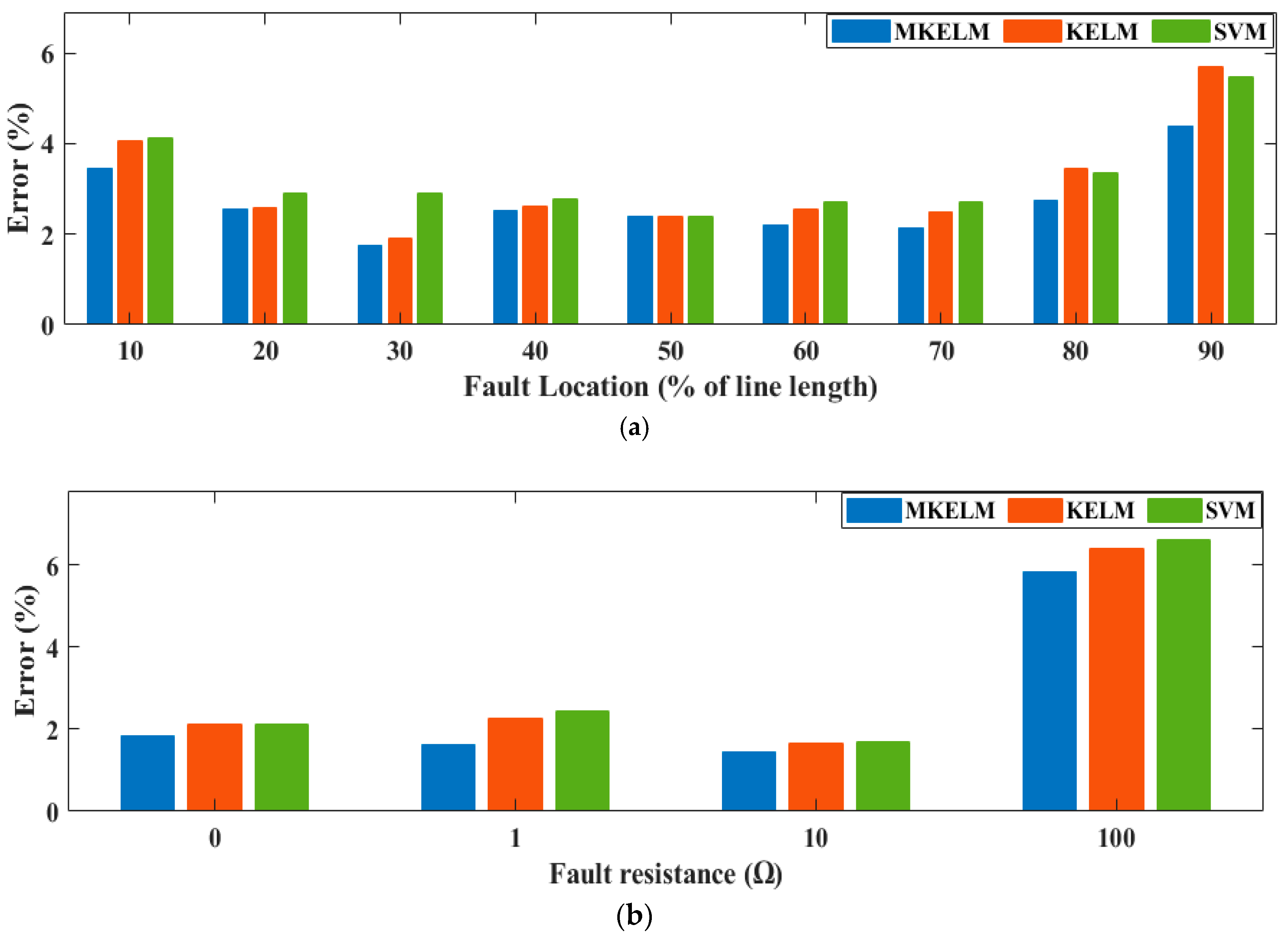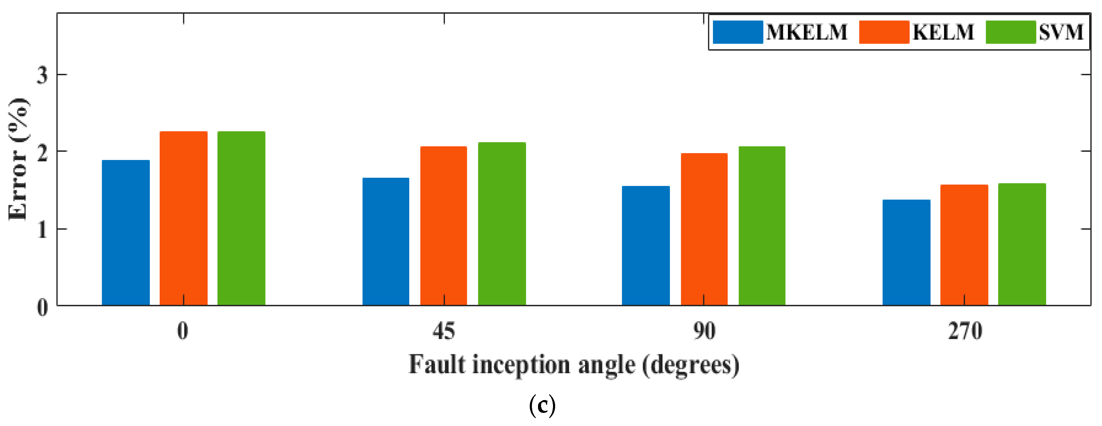The MKELM inherits the properties of the ELM; e.g., it exhibits extremely fast learning speed, good generalization performance, and is less prone to local minima and overfitting than gradient-based learning algorithms [33]. The parameters of the MKELM are optimized using a genetic algorithm (GA) to obtain good classification and location performance. A GA is used due to its simplicity and efficiency, it is easier to converge, and it gets a better global solution than other methods. The performance of the proposed method is tested for all types of faults for a wide range of operating and fault conditions with radial and loop microgrid topologies in the grid-tied and islanded modes. The performance of the proposed method is validated by comparing the results with those of single-kernel ELM (KELM)- and SVM-based methods and is evaluated with measurement noises in the current signals. The test results indicate that the MKELM achieves higher fault classification and location performance than the KELM and SVM.

The main contributions of this paper can be highlighted as follows:

• A non-redundant and efficient version of S-transform (DOST) is used for feature extraction from fault current signals.
• A multi-kernel ELM (MKELM) method is used as an intelligent fault detection, classification, and location method in a microgrid.
• A genetic algorithm (GA) is used for optimizing the parameters of MKELM in order to obtain good generalization performance.
• The development of a robust microgrid fault detection, classification, and location identification method applicable to both islanded and grid-tied mode of operation with radial and looped topologies of microgrids.

The remainder of this paper is organized as follows. Section 2 presents a brief overview of the DOST. Section 3 describes the studied microgrid test system. Section 4 discusses the proposed method. The simulation results are presented in Section 5, and conclusions are drawn in Section 6.

2. Discrete Orthonormal S-Transform

The S-transform is a time-frequency analysis method, which is extended from the short-time Fourier transform (STFT) and the wavelet transform [34]. The S-transform combines the absolute phase-retaining properties of the Fourier transform with the frequency-dependent analysis and multi-resolution properties of the wavelet transform. The continuous S-transform of a time-series signal x(t) with frequency f and time variable t and τ is defined as [34,35]:

$$S(\tau ,f)=S\{x(t)\}={\displaystyle \underset{-\infty }{\overset{\infty }{\int }}x(t)}\frac{\left|f\right|}{\sqrt{2\pi }}{e}^{-\frac{{(\tau -t)}^2{f}^2}{2}}{e}^{-j2\pi ft}dt$$

(1)

The discrete version of the S-transform, with time samples (p), frequency steps (n), and the total number of samples (N), can be expressed as [34,35]:

$$S\left[pT,\frac{n}{NT}\right]={\displaystyle \sum _{m=0}^{N-1}X\left[\frac{m+n}{NT}\right]} e^{- \frac{2{\pi }^2{m}^2}{n^2}} e^{\frac{j2\pi mp}{N}} ; n\ne 0$$

(2)

where n, p = 0, 1, 2, ..., N − 1 and $X\left[\frac{n}{NT}\right]$ is the DFT of the sampled signals x[mT] and given as [34,35]:

$$X\left[\frac{n}{NT}\right]=\frac{1}{N}{\displaystyle \sum _{m=0}^{N-1}x\left[mT\right]}{ \mathrm{e}}^{\frac{j2\pi nm}{N}}$$

(3)

The DOST is a non-redundant and efficient version of the S-transform that resolves many of the memory and computational issues of the S-transform [35]. The DOST reduces the redundancy of the S-transform by partitioning the output of the S-transform into N regions, each of which is represented by a coefficient. The DOST is represented by a set of orthonormal basis functions that localize the Fourier spectrum of the signal and retain the advantageous phase properties of the S-transform. The DOST coefficients can be computed using the inner products between sampled signals x[mT] and a set of orthonormal basis functions $S_{\nu ,\beta ,\tau }\left[mT\right]$ [34,35].

$$S\left[\tau T,\frac{\nu }{NT}\right]={\displaystyle \sum _{m=0}^{N-1}x\left[mT\right]}{S}_{\left[\nu ,\beta ,\tau \right]}\left[mT\right]$$

(4)

$$S_{\nu ,\beta ,\tau }\left[mT\right]=\frac{j{e}^{j\pi \tau }}{\sqrt{\beta }}\frac{\left\{e^{j2\pi \left(\frac{m}{N}-\frac{\tau }{\beta }\right)\left(\nu -\frac{\beta }{2}-\frac{1}{2}\right)}-e^{j2\pi \left(\frac{m}{N}-\frac{\tau }{\beta }\right)\left(\nu +\frac{\beta }{2}-\frac{1}{2}\right)}\right\}}{2\sin \left[\pi \left(\frac{m}{N}-\frac{\tau }{\beta }\right)\right]}$$

(5)

where ν is the center of a frequency band, β is the width of a frequency band, and τ is the location in time. The output of the DOST is an N × 1 complex vector that represents time-frequency efficiently, and the elements of the vector are linearly independent.

The main advantages of the DOST are its high computational efficiency, low memory requirements, immunity to measurement noise, and effectiveness for analyzing non-stationary signals such as fault voltage and current signals [36].

3. Microgrid Test System

The standard International Electrotechnical Commission (IEC) microgrid test system model was used in this study [37]. This system operates with base values of 25 kV, 15 MVA, and 60 Hz. It was simulated using MATLAB/Simulink, as shown in Figure 1. It consists of three inverter-based DERs (DER1, DER2, and DER3) and one synchronous generator-based DER (DER4). It can be operated in the grid-tied or islanded mode by switching the main circuit breaker (CB main) and can be operated with a radial or looped topology by switching CB Loops 1 and 2. The distribution lines are divided into five sections (DL-1–DL-5), each with a line length of 20 km. The loads (L-1–L-6) are distributed along with the microgrid test system. Figure 2 shows the variation of a fault current in the studied microgrids depending on the operating mode (grid-tied or islanded) and network configuration (radial or looped).

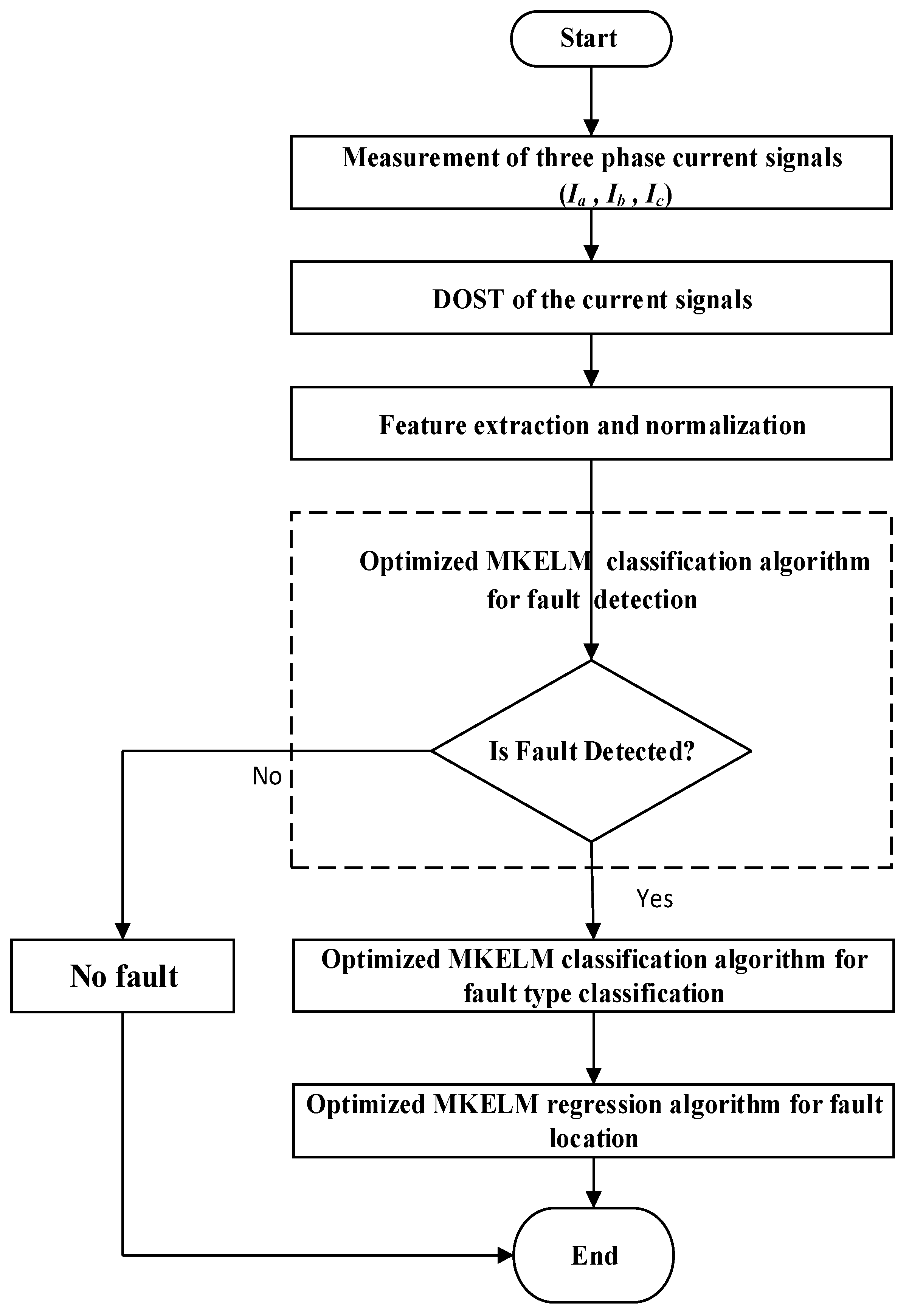
4. Proposed Method

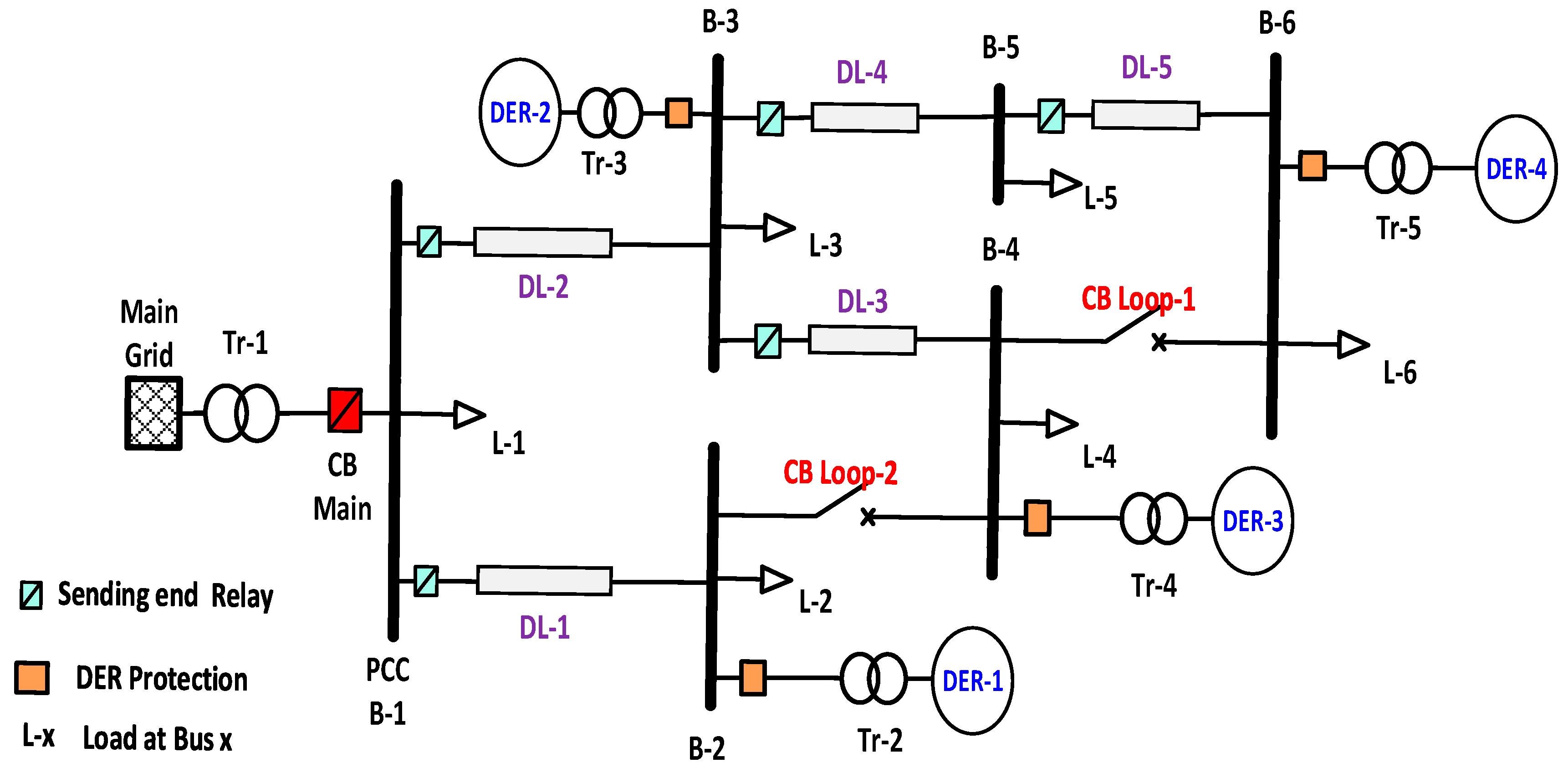
The proposed method, employing one cycle of post-fault current signals retrieved at the sending-end of each distribution line in the standard IEC microgrid system was applied for fault classification and location in the microgrid. The retrieved fault current signals were first filtered by a low-pass Butterworth filter and sampled with a sampling rate of 3.84 kHz (64 samples/cycle). A flowchart of the proposed method for fault detection, classification, and location identification is shown in Figure 3. The subsequent subsections explain the proposed method in detail.

4.1. Feature Extraction Using DOST

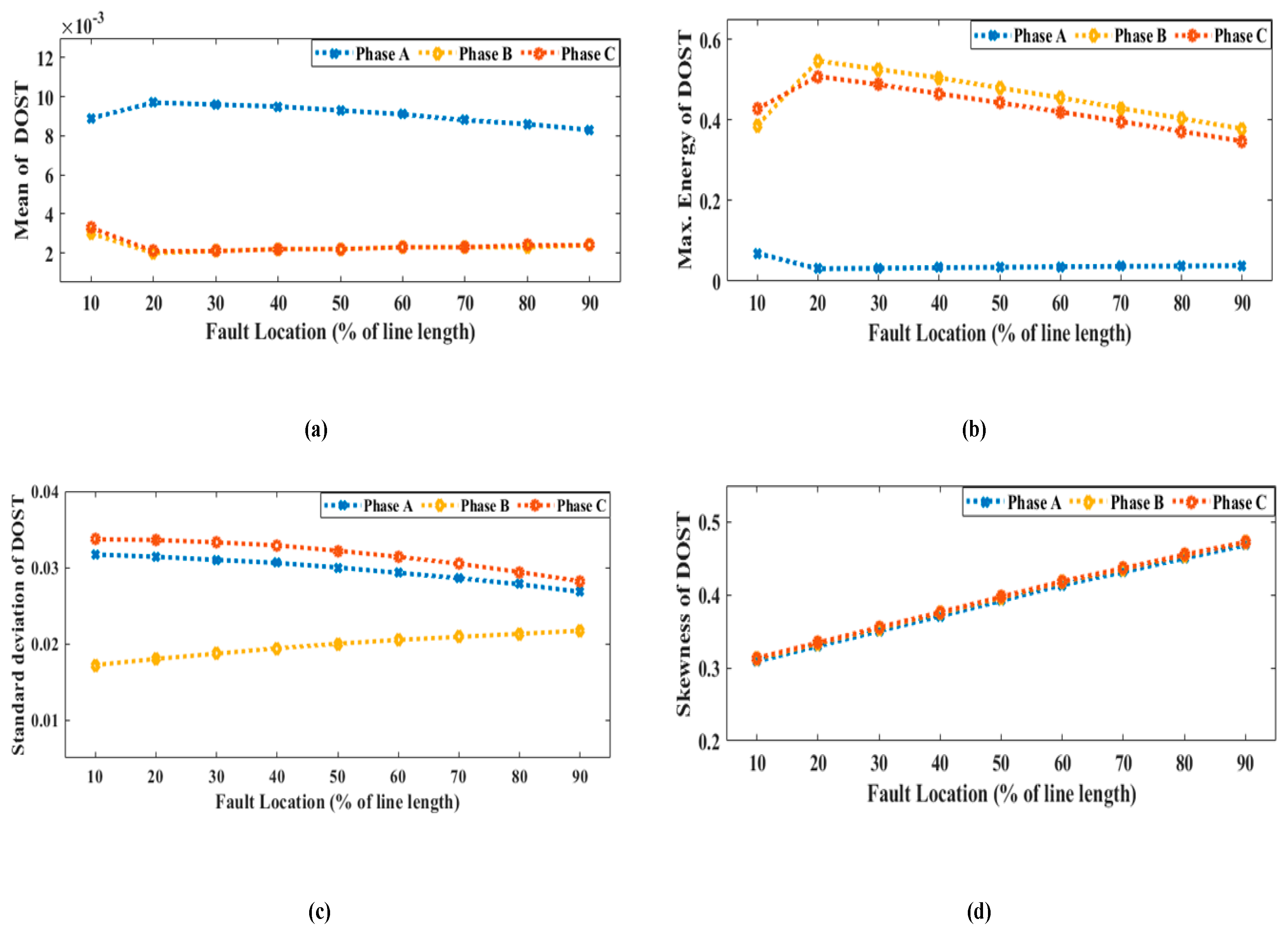
For fault classification and location, the one cycle post-fault current signals were processed through the DOST for feature extraction. The DOST output coefficient is a complex vector that can be represented by a magnitude and phase angle. Standard statistical methods, such as the mean, energy, standard deviation, entropy, kurtosis, and skewness, were applied to the magnitude and phase angle of the DOST coefficient to extract important features. In this study, among the different statistical features, five distinct features for each phase were selected according to their efficiency for the proposed method, through trial and error:

• Feature F1_x: Mean of the magnitude of the DOST.
• Feature F2_x: Maximum energy of the magnitude of the DOST.
• Feature F3_x: Standard deviation of the magnitude of the DOST.
• Feature F4_x: Skewness of the magnitude of the DOST.
• Feature F5_x: Standard deviation of the phase angle of the DOST.

Here, x represents the phase (a, b, or c). The features are normalized to improve the generalization and reduce the estimation error. 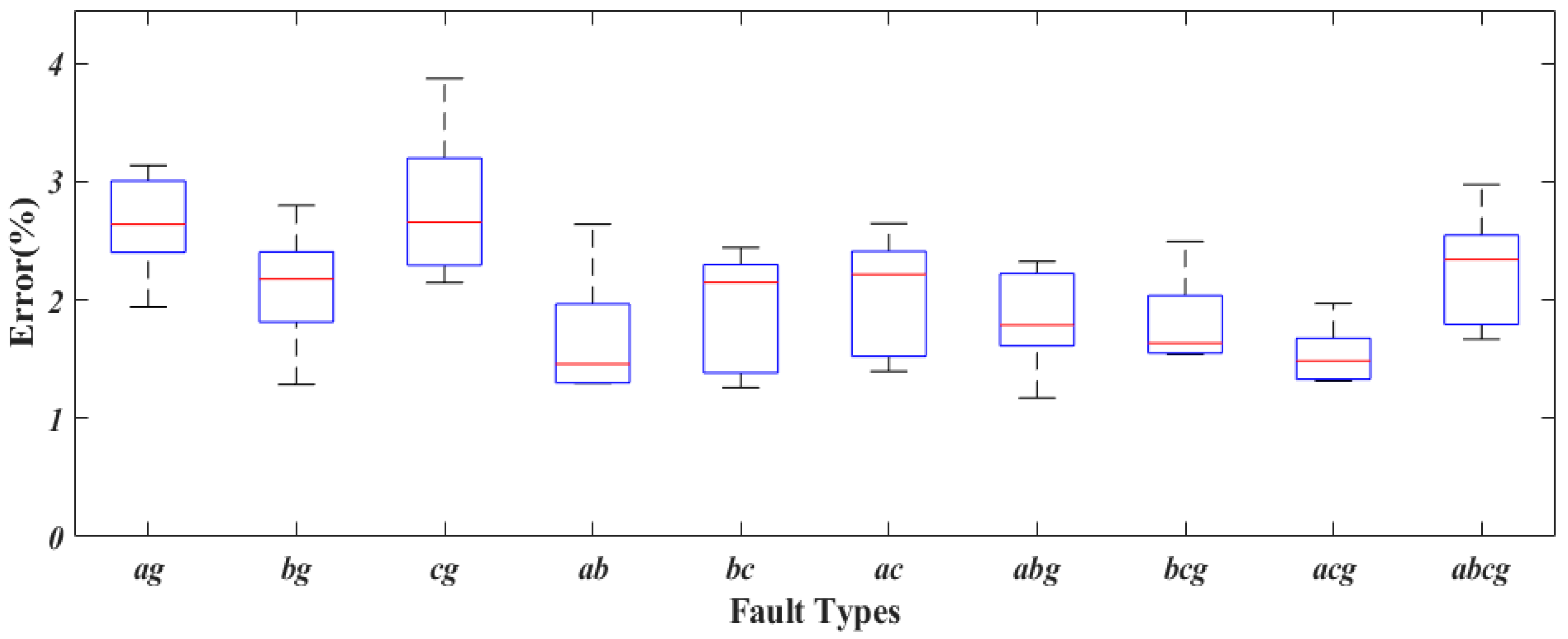The variation of these normalized fault features with respect to the fault location for a single line to ground (ag) and a double line to ground (bcg) faults in radial grid-tied mode and for a line to line (ac) and a three-phase (abcg) faults in looped islanded mode are presented in Figure 4a–d, respectively. It is shown from the figure that the features can easily distinguish the faulty phase from healthy phases and vary with fault locations.

4.2. Multi-Kernel Extreme Learning Machine

This subsection discusses the development of the MKELM for fault classification and location in a microgrid. The ELM is a type of single-hidden layer feedforward neural network that was proposed by Huang et al. [38]. It selects input weights and biases randomly and analytically determines the output weights instead of tuning iteratively. Figure 5 shows the architecture of standard ELM with input weights ω, bias b, hidden nodes L, and output weights α.

The standard ELM can be expressed mathematically as follows:

$$H\alpha =T$$

(6)

$$\begin{array}{l}H={\left[\begin{array}{l}{h}_1(x_1) \cdots h_L(x_1)\\ \hspace{1em}\hspace{1em}⋮\hspace{1em}\hspace{1em}⋮\hspace{1em}\hspace{1em}⋮\\ h_1(x_n) \cdots h_L(x_n)\end{array}\right]}_{n\times L}\\ \\ ={\left[\begin{array}{l}{G}_1({\omega }_{11}\cdot x_1+b_1) \cdots G_L({\omega }_{1L}\cdot x_1+b_L)\\ \hspace{1em}\hspace{1em}\hspace{1em}\hspace{1em}\hspace{1em}⋮\hspace{1em}\hspace{1em}\hspace{1em} ⋮\hspace{1em}\hspace{1em}\hspace{1em}\hspace{1em}⋮\\ G_1({\omega }_{n1}\cdot x_n+b_1) \cdots G_L({\omega }_{n1}\cdot x_n+b_L)\end{array}\right]}_{n\times L}\end{array}$$

(7)

where H is the hidden layer output matrix, α is the output weight matrix, T is the matrix of the target output, and G_L is the activation function used in each hidden neuron. The output weight (α) can be obtained by solving Equation (6) by using the Moore–Penrose generalized inverse of H:

$$\alpha =H^{†}T$$

(8)

To improve the stability of the ELM, we can rewrite (8) as:

$$\alpha =H^T{\left(\frac{1}{C}+H{H}^T\right)}^{-1}T$$

(9)

where C is the regularization parameter, and the output function of the ELM is given as follows:

$$y=h(x)\alpha =h(x)H^T{\left(\frac{1}{C}+H{H}^T\right)}^{-1}T$$

(10)

The ELM performance is improved by using a sum of different activation functions [39] or multiple kernel functions on hidden layer nodes [40].

A KELM is an ELM with kernel functions in the hidden layer nodes [41]. A kernel function is used to map the data in the input space to the high-dimensional feature space and converts a nonlinear problem into a linear problem. The kernel function can be defined using Mercer’s conditions for unknown feature mapping h(x):

$$\begin{array}{l}k(x_i,x_j)=h(x_i)\cdot h(x_j)\\ K=H{H}^T\end{array}$$

(11)

where k(x_i, x_j) is a kernel function and K is the kernel matrix. The output function of the KELM is obtained by substituting Equation (11) into Equation (10):

$$y=h(x)\alpha =\left[\begin{array}{l}k(x,x_1)\\ \hspace{1em}\hspace{1em}⋮\\ k(x,x_n)\end{array}\right]{\left(\frac{1}{C}+K\right)}^{-1}T$$

(12)

The generalization performance and learning ability of the KELM depend on the types of kernel function used in the hidden layer nodes. There are many types of kernel functions, which can be categorized into two main groups: Global and local. Global kernel functions, such as linear and polynomial kernel functions, have high generalization performance but a weak learning ability and are affected by samples far from each other. Local kernel functions, such as Gaussian and wavelet kernel functions, have a strong learning ability but low generalization performance and are affected by samples close to each other.

A linear combination of different kernel functions yields a multi-kernel function that satisfies Mercer’s conditions. An MKELM is obtained by using the multi-kernel function in the hidden nodes of the KELM. The multi-kernel function with a balancing parameter (λ) between different kernels is expressed as follows:

$$k(x_i,x_j)={\displaystyle \sum _{n=1}^N{\lambda }_n}{k}_n(x_i,x_j)$$

(13)

In this study, we investigated the effectiveness of the MKELM for the classification and location of faults in the microgrid by using two kernel functions—wavelet and polynomial:

$$\begin{array}{c}k(x_i,x_j)=\lambda k_1(x_i,x_j)+(1-\lambda )k_2(x_i,x_j)\\ 0 \le \lambda \le 1\end{array}$$

(14)

where k₁(x_i,x_j) is the Morlet wavelet kernel function, which is given as:

$$k_1(x_i,x_j)=\cos \left(1.75\left(\frac{x_i-x_j}{\gamma }\right)\right){ \mathrm{e}}^{-\frac{{\left(x_i-x_j\right)}^2}{2{\gamma }^2}}$$

(15)

and k₂(x_i,x_j) is polynomial kernel function, which is given as:

$$k_2(x_i,x_j)={\left(1+x_i\cdot x_j\right)}^d$$

(16)

Here, γ and d represent the dilation of the wavelet kernel and the polynomial degree, respectively. These parameters must be optimized for the MKELM to achieve good performance.

4.3. GA for Parameter Optimization

A GA is a biologically inspired optimization algorithm that mimics the natural evolution for finding optima of the problem. In contrast to classical optimization approaches, GAs are able to solve all kinds of objective functions such as continuous, discontinuous, integer, smooth, and non-smooth functions. In the GA, the optimization starts with generating a number of random solutions, known as the population of the GA. First, the initial population is evaluated, and the objective function values are recorded for the entire initial population. Second, the termination conditions of the algorithms are verified if the current generation does not meet the termination conditions. In the second stage, the selection is performed, and the best solutions from the population are moved to the next generations. The process depicts the survival of the fittest phenomenon. After selection, the crossover operation is performed on the newly selected population. In the crossover, two-parent solutions are picked randomly from the population, and some of the portions of parent solutions are exchanged to generate offspring; the operation increases the diversity in the population. Finally, after crossover, a mutation operation is applied to the population to introduce diversity. However, the probability of mutation is kept small to avoid destruction in the quality of the solutions. The execution of all the above steps is carried out before evaluating the fitness again, and the whole population through the above steps is known as a generation. The process terminates if the stopping criteria, such as a maximum number of generations or no further improvement in the fitness value, meet the required settings. This completes the optimization process of the GA and provides the optimal solution.

A GA was employed in this study for optimization of the parameters (including the regularization parameter (C), dilation of the wavelet kernel (γ), polynomial degree (d), and balancing parameter (λ)). The ranges of the parameters employed in the optimization are presented in

Table 1. Parameters of the MKELM.

Parameter	Range
Regularization parameter (C)	[10−2, 1010]
Dilation of wavelet kernel (γ)	[10−4, 102]
Polynomial degree (d)	[1, 10]
Balancing parameter (λ)	[0, 1]

. The classification accuracy and relative error of the MKELM classification and regression algorithms were used as fitness functions [42,43].

5. Simulation Results

To evaluate the fault classification and location performance of the proposed method, various simulation studies were performed using a standard IEC microgrid test system in MATLAB/Simulink. For the performance evaluation, fault scenarios with various fault types, resistances, locations, inception angles, and topologies (radial and looped) were considered. Additionally, the performance of the proposed method was compared with that of KELM- and SVM-based methods. For both the KELM- and SVM-based methods, a Gaussian radial basis function kernel was used, and the parameters were optimized using a GA. Furthermore, the effect of measurement noise on the fault classification and location performance was investigated. The performance evaluation of the proposed methods is described in detail in the following subsections.

5.1. Fault Detection and Classification Performance

For evaluating the fault-detection performance of the proposed method, 288 non-faulty cases were generated by considering different parameters in the standard IEC microgrid test system, as shown in

Table 2. Condition for simulating no-fault cases.

Parameter Details	Count
Abrupt load change	6
Operating mode (grid-tied or islanded)	2
Topology (radial or looped)	2
Capacitor switching at load buses and point of common coupling (PCC)	6
Various DER penetration levels	2
Total no-fault cases	288

. A similar number of faulty cases were generated by varying the fault types, locations, resistances, and inception angles, along with the operating mode (grid-tied or islanded) and topology (radial or looped). Features were extracted from the total number of cases (faulty and non-faulty), as previously mentioned, and each case was labeled as either 1 (faulty) or 0 (non-faulty). The datasets were randomly divided into subsets for training and testing (70% and 30%, respectively) the MKELM classification algorithm. The MKELM classifies the faulty cases from non-faulty cases with 100% testing accuracy.

After fault detection, the fault classification performances were evaluated by considering different fault cases, as shown in

Table 3. Condition for simulating fault cases.

Parameter Details	Count
Topology (radial or looped)	2
Operating mode (grid-tied or islanded mode)	2
Fault types	10
Fault resistance (0.01, 1, 10, or 100 Ω)	4
Fault line (DL-1–DL-5)	5
Fault location (10%, 20%, · · ·, or 90% on fault line)	9
Fault inception angle (0°, 45°, 90°, 270°)	4
Total fault cases	28,800

. The classification of the fault types in a microgrid is a very important requirement for fault analysis and accurate fault location identification. All shunt type of faults were considered in this study, such as single line to ground fault (ag, bg, and cg), line to line fault (ab, bc, and ac), double line to ground fault (abg, bcg, and acg), and three phase to ground fault (abcg).

Features were extracted from the total number of fault cases, as previously mentioned, and labeled the fault types (ag, bg, cg, ab, bc, ac, abg, bcg, acg, and abcg) with a number from 1 to 10, respectively. The fault classification accuracy was evaluated by randomly dividing the datasets into subsets for training and testing (70% and 30%, respectively) the proposed method at each distribution line.

Table 4. Confusion matrix of the proposed method for fault classification.

	ag	bg	cg	ab	bc	ac	abg	bcg	acg	abcg
ag	854	0	0	2	1	0	2	3	0	0
bg	0	876	0	0	0	0	0	4	0	0
cg	1	0	843	0	1	3	0	2	4	0
ab	1	2	1	817	0	0	4	3	0	1
bc	0	0	0	0	869	0	1	5	1	3
ac	3	0	2	0	0	842	0	0	1	0
abg	1	1	0	3	1	0	847	0	0	2
bcg	0	3	1	0	4	0	1	834	0	3
acg	1	1	2	0	0	1	0	0	839	0
abcg	1	0	0	1	1	0	1	2	1	896
Overall Accuracy: 99.04%

presents the overall confusion matrix obtained from the MKELM classification algorithm. In the confusion matrix, the diagonal elements represent the number of correctly classified faults, and the off-diagonal elements represent the number of misclassified faults.

The proposed method was compared with KELM- and SVM-based methods with regard to the testing classification accuracy at each distribution line in the standard IEC microgrid system, as shown in

Table 5. Comparison of the fault-classification accuracy for the standard IEC microgrid system. KELM, single-kernel ELM; SVM, support vector machine.

MG Line	Classification Accuracy (%)
	MKELM	KELM	SVM
DL-1	99.48	99.42	98.90
DL-2	98.95	98.84	98.78
DL-3	98.84	98.43	98.37
DL-4	99.94	99.77	99.48
DL-5	97.97	97.27	97.50
Average	99.04	98.75	98.61

. The results indicate that the MKELM performed better than the KELM and SVM.

5.2. Fault Location Performance

After the fault classification, we evaluated the fault location performance of the proposed method by considering different cases for each type of fault, as shown in Table 3. The fault location performance was evaluated for each type of fault in all distribution lines. The percentage error for each fault type was used to evaluate the performance of the proposed method:

$$\%Error=\frac{\left|Output fault location-True fault location\right|}{Length of the distribution line}\times 100$$

(17)

The percentage error of the fault location was determined by randomly dividing the dataset of each fault type into subsets for training and testing (70% and 30%, respectively) the MKELM regression algorithm at each distribution line. The proposed method achieved an error between 1.17 and 3.87% with an overall mean error of 2.06%, as shown in Figure 6.

The fault location performance of the proposed method was compared with that of the KELM- and SVM-based methods with regard to the average percentage error at each distribution line in the standard IEC microgrid system, as shown in

Table 6. Comparison of the fault location error in the standard IEC microgrid system.

MG Line	Error (%)
	MKELM	KELM	SVM
DL-1	2.27	2.57	2.66
DL-2	1.75	2.03	2.06
DL-3	2.38	2.77	2.81
DL-4	1.60	1.84	1.86
DL-5	2.32	2.56	2.62
Average	2.06	2.35	2.40

. The results indicate that the MKELM had a smaller fault location percentage error than the KELM and SVM.

The fault location performance of the proposed method was evaluated and compared with that of the KELM- and SVM-based methods with the variation of the fault location, fault resistance, and fault inception angle (FIA). Figure 7 presents the average percentage errors of the MKELM, KELM, and SVM with variations of the fault location, fault resistance, and FIA for single line to ground (ag) faults. The fault location percentage errors varied with respect to the fault distance measured from the sending-end relay of the distribution lines. As shown in Figure 7a, a large percentage error occurred near the end of the distribution lines. Figure 7b shows the effect of the variation of the fault resistance on the fault location percentage errors; a large percentage error occurred at the high-impedance fault (100 Ω). Figure 7c shows that the percentage errors varied with respect to the FIA, and a large percentage error occurred at an FIA of 0°. In all cases, the MKELM had a smaller percentage error than the KELM and SVM.

5.3. Effect of Noise

The robustness of the proposed method was tested in the presence of measurement noise in the current signals. For this, 30- and 40-dB signal-to-noise ratio (SNR) white Gaussian noise signals were added to one cycle of post-fault current signals measured from the sending-end of each distribution line, considering the same cases shown in Table 3. Under this condition, the fault classification and location performance of the proposed method were still better than that of KELM and SVM for different types of faults in the standard IEC microgrid system, as shown in

Table 7. Effects of noise on classification and location performance.

SNR	Classification Accuracy (%)			Error (%)
	MKELM	KELM	SVM	MKELM	KELM	SVM
30 dB	98.29	98.15	98.24	2.53	2.64	2.65
40 dB	98.73	98.59	98.38	2.31	2.60	2.62

, although the performance deviated slightly from that without noise (Table 5 and Table 6).

6. Conclusions

This paper proposes a new method for fault classification and location identification in a microgrid using DOST-based optimized MKELM. The proposed method first extracts useful features from the magnitude and phase angle of the DOST output coefficient by preprocessing one cycle of post-fault current signals retrieved from sending-end relays of microgrids. Then, the features are normalized and used as an input to the MKELM. We used MKELM with a combination of two different types of kernels, i.e., wavelet kernel and polynomial kernel, in the hidden nodes of the ELM to classify and locate the faults in the microgrid. A GA was used to optimize the parameters of the MKELM. The performance of the proposed method was tested on the standard IEC microgrid test system for various operating conditions and fault cases, including different fault locations, fault resistance, and FIAs. The simulation results indicate that the proposed method can detect, classify, and locate any type of fault in a microgrid with high performance. Furthermore, the simulation results obtained with measurement noise in the current signals confirm the robustness of the proposed method.