Study on the Interaction Mechanism of Hydraulic Fracture and Natural Fracture in Shale Formation

Abstract

Hydraulic fracturing is an essential technique for the development of shale gas, due to the low permeability in formation. Abundant natural fractures contained in a formation are indispensable for the development of a fracture network. In this paper, a damage-stress-seepage coupled hydraulic fracture expansion model, based on the extended finite element method, is established. The simulation results show that shear failure occurs when the hydraulic fracture interacts with a frictional natural fracture, while tensile failure occurs when it interacts with a cement natural fracture. Low interaction angles and high tensile strength of the rock are beneficial for the generation of a complex fracture network. Furthermore, under the same geological conditions and injection parameters, frictional natural fractures are more beneficial for the generation of a complex fracture network, when compared with cement natural fractures. This can not only effectively increase the propagation length of the natural fracture, but also effectively reduce its reactive resistance. This research is of great significance for the efficient exploitation of unconventional oil and gas resources.

1. Introduction

Hydraulic fracturing is an important technique for shale reservoirs and the exploitation of tight sand reservoirs [1,2]. A single planar fracture is insufficient for the successful economic extraction of an unconventional resource, and a complex fracture network is necessary to achieve economic development [3,4]. Due to a large number of natural fractures (NFs) existing in shale formations, which has a great effect on the hydraulic fracture (HF) propagation [2,5,6,7], it is necessary to correctly predict the development of a complex fracture network during fracturing treatments, in order to optimize stimulation designs and completion strategies.

Theoretical and experimental investigation are the main methods used to analyze the interactions between natural fractures and the hydraulic fracture. Experimental results indicate that a hydraulic fracture can cross the weak plane when it comes across a natural fracture, and that a natural fracture cannot change the direction of propagation of the hydraulic fracture [8,9,10,11,12]. Furthermore, the experimental results suggest that the approach angle, the strength of the natural fracture, and the difference in the principal stress are the three predominant factors that affect fracture propagation when a hydraulic fracture comes across a natural fracture [13]. Some experiments demonstrated that the treatment parameters of hydraulic fracturing also have a great effect on the propagation of a hydraulic fracture when it comes across a natural fracture, where increasing the injection rate or fracturing fluid viscosity can increase the possibility that a hydraulic fracture will come across a natural fracture [14,15,16]. Limited by the theoretical and experimental investigations, numerical simulations play an important role in understanding the interactions between natural fractures and hydraulic fractures. The displacement discontinuity method (DDM) [17,18], the distinct element method (DEM) [19,20,21,22,23], and the finite element method (FEM) [5,19,20] are the most widely used numerical techniques for modeling hydraulic fracturing. However, there exist some difficulties in modeling fracture propagation in a fractured formation. As the fracture extension trajectory is predefined in DDM, it cannot simulate the fracture deflection caused by induced stress. Although the DEM can effectively simulate the interaction process between a hydraulic fracture and a natural fracture, it is difficult to describe the actual dynamics of hydraulic fracture and natural fracture propagation, due to the extensive calculations required and an inability to consider the formation of new fractures in the simulation process. The extended finite element is a promising method for the simulation of fracture propagation, as it does not pre-define the fracture propagation trajectory; thus, it can effectively simulate the fracture deflection caused by stress field alternation. In addition, it avoids mesh updating in the calculation, such that the calculation efficiency can be improved greatly. Furthermore, interactions between natural fractures and the hydraulic fracture can be effectively simulated. Thus, the extended finite element method was selected to simulate the fracture interaction in fractured formation in this paper.

On the basis of the extended finite element theory and the cohesive element method, a two-dimensional (2D) fracture propagation model which simulates hydraulic fracture propagation in a fracture formation is established. In this research, natural fractures are divided into two different types corresponding to two different failure modes. The different interaction criteria between NFs and HFs are demonstrated in the model. This research is of great importance for investigating the interaction mechanisms involved when a hydraulic fracture propagates in a fractured formation, which can help us to understand the formation mechanisms of complex fracture networks.

2. Methodology

2.1. Governing Equations

As indicated in Figure 1, a 2D homogeneous medium ($\mathsf{\Omega }$) contains a natural fracture $\mathrm{NF}$, which can interact with the $\mathrm{HF}$. The prescribed tractions t and the displacements $\overline{\mathbf{u}}$ are imposed on the boundary (${\mathit{\Gamma }}_{\mathit{t}}$ and ${\mathit{\Gamma }}_{\mathbf{u}}$, respectively). For simplicity, it is assumed that the fluid is incompressible and that the propagation of the fracture is a quasi-static process. The fracturing fluid leak-off into the matrix is considered by the Carter leak-off model.

The equilibrium equation of the domain and the boundary conditions can be expressed as

$$\{\begin{array}{c}\nabla ·\sigma +b=0 in \mathsf{\Omega }\\ u=\overline{u} on {\mathsf{\Gamma }}_u\\ \begin{array}{c}\sigma ·n=t on {\mathsf{\Gamma }}_t\\ \begin{array}{c}\sigma ·n_{{\mathsf{\Gamma }}_{HF}}=p{n}_{{\mathsf{\Gamma }}_{HF}} on {\mathsf{\Gamma }}_{HF}\\ \sigma ·n_{{\mathsf{\Gamma }}_{NF}}=t^{cont} on {\mathsf{\Gamma }}_{NF}\end{array}\end{array}\end{array},$$

(1)

where $\sigma$ is the Cauchy stress tensor, $b$ is the body force, $p$ is the fluid pressure, and $t^{cont}$ is the traction acting on the surface of the NF and HF.

2.2. Fracture Propagation Criterion

The fracture propagation criterion, based on linear elastic fracture mechanics (LEFM), assumes that there is a fracture process zone near the fracture tip. Compared with the fracture size, the material shows very little inelastic behavior. Fracture propagation occurs when the stress intensity factor exceeds the material strength. Nevertheless, the adequacy of this assumption is questionable, as fracture propagation in quasi-brittle and ductile materials leads to significant plastic deformation around the fracture tip due to a shared failure. In addition, even for brittle materials, the fracture course area can become concentrated at a single point, and initial cracks need to exist for LEFM to apply [13,14]. The bond zone model is a simple model which is suitable for processing zones and materials that fail as a result of crack propagation and coalescence.

The constitutive behavior of the viscous region is defined by the traction–separation relationship. The elastic behavior is represented by an elastic constitutive matrix, which links the normal stress and shear stress with the normal and shear separation of crack elements.

$$t=\left\{\begin{array}{c}{t}_n\\ t_s\\ t_t\end{array}\right\}=\left[\begin{array}{ccc}{K}_{nn}& 0& 0\\ 0& K_{ss}& 0\\ 0& 0& K_{tt}\end{array}\right]\left\{\begin{array}{c}{\delta }_n\\ {\delta }_s\\ {\delta }_t\end{array}\right\}=K\delta .$$

(2)

The nominal traction stress vector $t$ consists of the components $t_n$, $t_s$, and $t_t$, which represent the normal and the two shear tractions, respectively. The corresponding separations are denoted by ${\delta }_n$, ${\delta }_s$, and ${\delta }_t$.

Damage modeling can be used to simulate the degradation and ultimate failure of the strengthening elements. The failure mechanism consists of two parts: the damage initiation criterion and the damage evolution law. In this law (Figure 2), the element does not undergo damage under pure compression unless the traction reaches the cohesive strength $T_0$ or if the separation reaches the displacement of damage ${\delta }_0$. When $\delta$ exceeds ${\delta }_0$, the traction decreases to 0 as the displacement increases and the cohesive element is completely damaged.

The damage initiation criterion is defined as follows:

$$f={\left\{\frac{\langle t_n\rangle }{t_n^0}\right\}}^2+{\left\{\frac{t_s}{t_s^0}\right\}}^2+{\left\{\frac{t_t}{t_t^0}\right\}}^2,$$

(3)

where $t_n$ is the stress in the nominal stress (Pa), $t_s$ is the stress in the first shear direction (Pa), $t_t$ is the stress in the second shear direction (Pa), $t_n^0$ is the peak value stress in the nominal stress (Pa), $t_s^0$ is the peak value in the first shear direction (Pa), and $t_t^0$ is the peak value in the second shear direction (Pa). The Macaulay bracket < > in the normal direction signifies that pure compression does not initiate damage.

2.3. Damage Evaluation

The damage evolution law describes the rate at which the material stiffness is degraded once the corresponding initiation criterion is reached. In this model, the damage law is described as follows:

$$t_n=\{\begin{array}{c}\left(1-D\right)\overline{t_n}, \overline{t_n}\ge 0\\ \overline{t_n},\overline{t_n}<0\end{array},$$

(4)

$$t_s=\left(1-D\right)\overline{t_s},$$

(5)

$$t_t=\left(1-D\right)\overline{t_t},$$

(6)

where D is the overall damage in the material and captures the combined effects of all the active mechanisms; the initial value of D is 0. If the evolution of the damage is modeled, D monotonically evolves from 0 to 1 after the damage starts and further loads. The parameters $\overline{t_n}$, $\overline{t_s}$, and $\overline{t_t}$ are the stress components predicted by the elastic traction separation behavior of the current strain without damage.

$$D=\frac{{\delta }_m^f\left({\delta }_m^{max}-{\delta }_m^0\right)}{{\delta }_m^{max}\left({\delta }_m^f-{\delta }_m^0\right)},$$

(7)

where ${\delta }_m=\sqrt{{\langle {\delta }_n\rangle }^2+{\delta }_s^2+{\delta }_t^2}$, ${\delta }_m^0$ is the effective displacement at damage initiation, and ${\delta }_m^{max}$ is the maximum value of the effective displacement attained during the loading history.

2.4. Fluid Flow within the Fractures

In the model, the leakage of fracturing fluid from the fracture to the matrix is considered. The Biot theory is employed in an updated Lagrangian framework. The governing equations of a deformable porous medium are presented for the solid–fluid mixture in the framework of Biot’s theory [24], and the fluid flow in the fracture and the proppant transport within the fracture are controlled by a UMAT (user-defined material mechanical behavior) subroutine [25,26].

$$\nabla ·\sigma -\rho \ddot{u}+\rho b=0,$$

(8)

$$\nabla ·\left[k_f\left(-\nabla p-{\rho }_f\ddot{u}+{\rho }_{f}b\right)\right]+\alpha \nabla ·\dot{u}+\frac{1}{Q}\dot{p}=0.$$

(9)

The fluid flow through the discontinuity is modeled by the continuity equation for the fluid flow within the fracture, which can be written according to Equation (10).

$$\nabla ·\dot{w}+ \alpha \nabla ·\dot{u}+\frac{1}{k_f}\dot{p}=0.$$

(10)

For a viscous fluid flow with Newtonian rheology, the fracture permeability is estimated, using the cubic law, as follows:

$$k_f=\frac{1}{\beta }\frac{w^2}{12{\mu }_f}.$$

(11)

The Carter leak-off model [18] is introduced to describe the normal flow of hydraulic fracturing. In the simulation, the leak-off of the fracturing fluid through the fracture faces into the surrounding medium is calculated by the Carter leak-off model.

The normal flow rates at the top and bottom sides of the cohesive element are defined as

$$\{\begin{array}{c}{q}_t=c_t\left(p_i-p_t\right)\\ q_b=c_b\left(p_i-p_b\right)\end{array}.$$

(12)

According to the fluid mass balance, at a certain period, part of the injected fluid fills the fracture and the rest is lost to the rock matrix, as shown in the following equation:

$$\frac{\partial d}{\partial t}+\nabla ·q+\left(q_t+q_b\right)=q_{inj}\delta \left(x,y\right).$$

(13)

Then, the control equation of the rock matrix involves coupling the fluid flow and rock deformation, as follows:

$${\sigma }_{ij}-{\sigma }_{ij}^0=\frac{E}{1+v}\left({\epsilon }_{ij}+\frac{v}{1-2v}{\epsilon }_{kk}{\delta }_{ij}\right)-\alpha \left(p_w-p_w^0\right){\delta }_{ij},$$

(14)

where $b$ is the body force, $\mathsf{\rho }$ is the average density of the solid–fluid mixture, ${\rho }_f$ is the density of the fracturing fluid, $p$ is the total fluid pressure, $Q$ is the pump ratio, $w$ is the fracture width, $c_t$ and $c_b$ are the leak-off coefficients of the top and bottom faces of the element, respectively, and $p_i$, $p_t$, and $p_b$ are the inner pressure of the element, the pressure of the top face, and the pressure of the bottom face, respectively.

2.5. The Extended Finite Element Method

Crack propagation is described by the Heaviside step function and the two-dimensional linear elastic progressive crack-tip displacement field. Relative to the basic finite element mesh, the locations of fracture discontinuities can be arbitrary, and the fracture propagation simulation can be carried out without changing as the fracture advances. For a displacement vector function u, the unit enrichment partition is approximated by

$$u={\displaystyle \sum }_{i=1}^N{N}_i\left(x\right)[u_i+H\left(x\right)a_i+{\displaystyle \sum }_{\alpha =1}^4{F}_{\alpha }\left(x\right)b_i^{\alpha }],$$

(15)

where $N_i\left(x\right)$—the first term on the right-hand side—is the normal nodal shape function, $u_i$ is a common nodal displacement vector associated with the continuous part of the finite element solution, $a_i$ is the product of the nodal enriched degree-of-freedom vector, $H\left(x\right)$ is the Heaviside function, $b_i^{\alpha }$ is the product of the nodal enriched degree-of-freedom vector, and $F_{\alpha }\left(x\right)$ represents the associated elastic asymptotic fracture-tip functions. The first term on the right-hand side is applicable to all nodes in the model, the second term is valid only for nodes whose shape function support is cut by the fracture interior, and the third term is used only for nodes whose shape function support is cut by the fracture tip.

The asymptotic fracture-tip functions $F_{\alpha }\left(x\right)$ are given by

$$F_{\alpha }\left(x\right)=\left[\sqrt{r}sin\frac{\theta }{2}, \sqrt{r}cos\frac{\theta }{2}, \sqrt{r}sin\frac{\theta }{2}sin \theta , \sqrt{r}cos\frac{\theta }{2}sin\theta \right],$$

(16)

where $\left(r,\theta \right)$ represents a polar co-ordinate system with origin at the fracture tip, and $\theta =0$ is tangential to the fracture at the tip. These functions span the elastostatic asymptotic fracture-tip function, where $\sqrt{r}sin\frac{\theta }{2}$ accounts for the discontinuity on the fracture face.

The level set method is used to track mobile interfaces and describe interfaces in the domain. In this method, the real interface is treated as a new interface with the same order as the original domain. In this paper, the interface is represented by a zero-order set of functions one dimension higher than the dimension of the interface, which evolves by solving the hyperbolic conservation law. The most common level set function is the signed distance function, which is used to represent the location of the interface.

$$\phi \left(x\right)=\Vert x-x^{*}\Vert sign\left({\mathbf{n}}_{{\mathsf{\Gamma }}_d}·\left(x-x^{*}\right)\right),$$

(17)

where $x^{*}$ is the closest-point projection of $x$ onto the discontinuity ${\mathbf{n}}_{{\mathsf{\Gamma }}_d}$, ${\mathbf{n}}_{{\mathsf{\Gamma }}_d}$ is the normal vector to the interface at the point $x^{*}$, $\Vert \Vert$ denotes the Euclidean norm, and $\Vert x-x^{*}\Vert$ specifies the distance from the point $x$ to the discontinuity ${\mathsf{\Gamma }}_d$.

In Equation (15), the symbols on both sides of the closed interface are different. With this definition, the discontinuity can be implicitly expressed as the zero-level contour of the level set function.

$$\mathrm{H}\left(\phi (x\right))=\{\begin{array}{c}-1 if \phi \left(x\right)<0\\ 1 if \phi \left(x\right)>0\end{array}.$$

(18)

2.6. Discretization of Governing Equations

By substituting the approximation in Equation (15) into the weak form of the equilibrium equation, the discretized form of the equilibrium equation can be obtained.

$$\mathrm{KU}-\mathrm{QP}-F^{ext}=0.$$

(19)

To approximate the one-dimensional pressure field inside the hydraulic fracture, the hydraulic fracture interface is discretized into fluid elements, as shown in Figure 3, and the pressure field can be approximated by the finite element method; that is,

$$p\left(s\right)={\displaystyle \sum }_{I\in S_{hf}}{N}_I^P\left(s\right)P_I.$$

(20)

By substituting Equation (20) into Equation (13), the discretized form of the fluid flow equation is derived as

$$Q^T\Delta U+\Delta tHP+\Delta tS=0,$$

(21)

where $K$ is the global stiffness matrix, $U$ is the global nodal displacement, $P$ is the nodal pressure vector, $Q$ is the coupling matrix, $F^{ext}$ is the external loading vector, and $H$ is the flow matrix.

2.7. The Fluid–Solid Coupling Method

The hydraulic fracturing model presented in this research involves three physical processes: (1) deformation of rock surface, (2) hydraulic fracture propagation induced by the hydraulic pressure, and (3) interaction between natural fractures and the hydraulic fracture. The coupled problem can be solved by three main steps during each time step. The first step involves determining the state of each fracture, i.e., whether the HFs are driven by fluid and the contact status of each NF. The Newton–Raphson iterative method based on the penalty method is adopted to solve the discretized non-linear equilibrium equation to determine the contact status. The second step involves iteratively solving the coupling between the deformation of HFs and the fluid flow within the fractures using the Newton–Raphson method. The third step involves calculating the stress state of each fracture tip; then, the location of each fracture tip is updated according to the crack propagation criterion. Figure 4 shows the flow chart of the coupled approach within each time step.

3. Simulation and Results

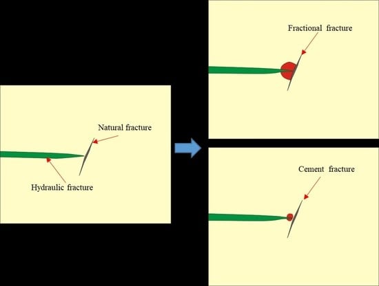
3.1. Verification

The published experimental results in Reference [19] were used to verify the effectiveness of the model. To improve the model’s computing speed, a 2D hydraulic fracturing model with coupled fracture surface deformation and pore pressure was proposed (see Figure 2). The dimensions of the model were 100 × 100 m², the length of the natural fracture was 6.0 m, and the injection position of the fracturing fluid was located at the left edge of the model. 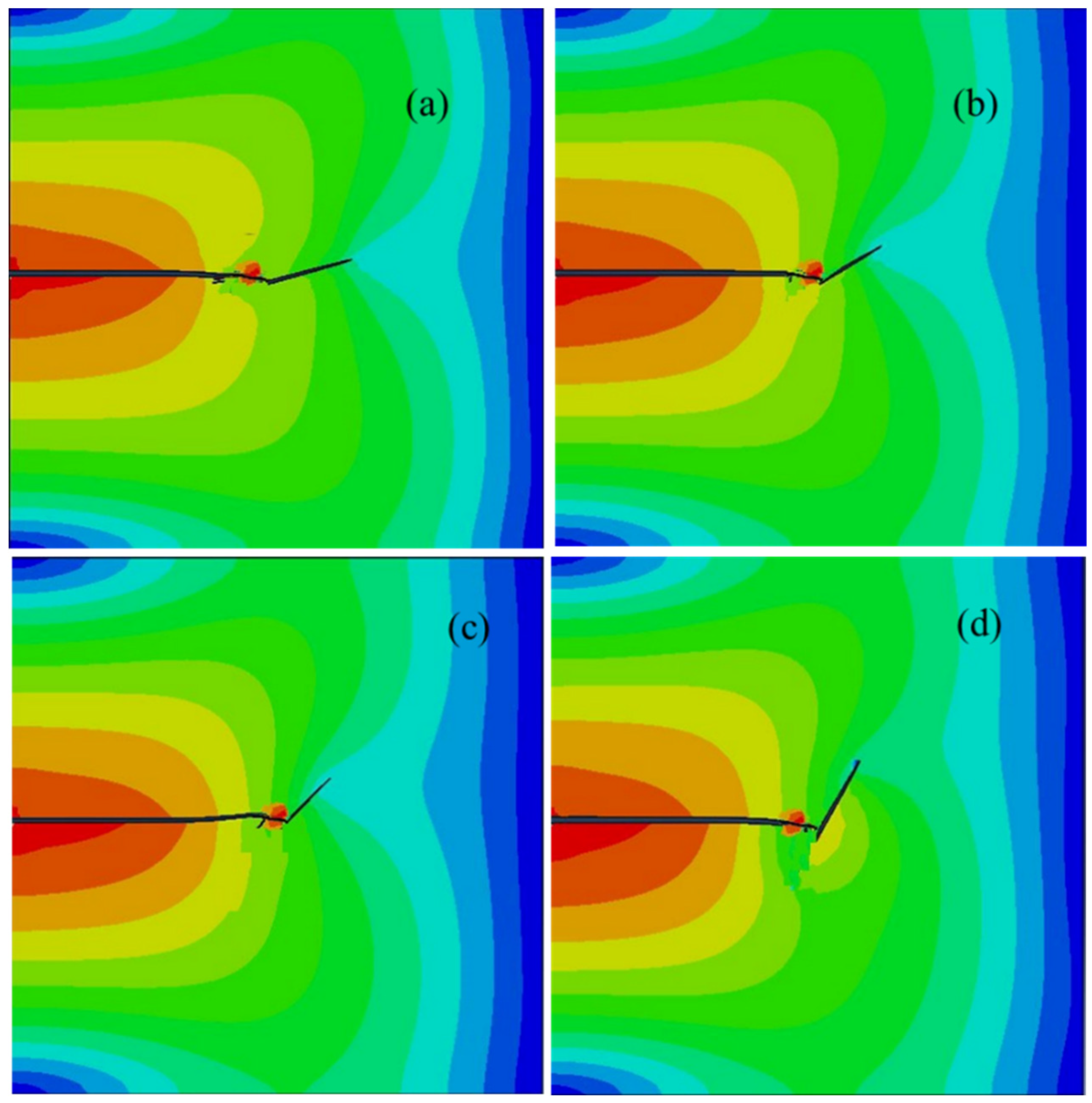The Young’s modulus E and Poisson’s ratio $v$ were 21.6 GPa and 0.28, respectively. The tensile strength of the rock sample was 6.28 MPa, and the other parameters of the model were consistent with the experiment. The simulation was considered completed when the HF came across the NF. The effective stress distribution around the fractures with an interaction angle of 45° is shown in Figure 5. When the stress difference was 7.0 MPa, it is evident that a stress concentration formed at the tip of the hydraulic fracture, which demonstrates that no shear slip occurred along the natural fracture surface. When the stress difference was decreased to 4.5 MPa, the stress concentration mainly appeared along the natural fracture surface; thus, it can be concluded that a slip failure occurred along the natural fracture surface. From the extended Renshaw and Pollard criterion [20], the interaction between the HF and NF can be predicted, and the comparison results between numerical simulations and experimental results are shown in Figure 6. The comparison indicates that the numerical results were consistent with the experimental results.

3.2. HF Interaction with Frictional NF

In the simulation, the four edges of the model were fixed, and the initial porosity of the model was 3.7%. It was assumed that the reservoir was homogeneous, and the natural fracture was closed completely. The dimensions of the model were 100 × 100 m², and the injection position of fracturing fluid was at the middle of the left edge. The frictional NF, with a length of 6 m, was located in the middle of the model, in order to effectively decrease the boundary effect caused by the model size. The other parameters in the model are shown in

Table 1. Key parameters of hydraulic fracturing model. NF—natural fracture.

Parameters	Value
Young’s modulus (E)	30.5 GPa
Poisson’s ratio ($v$)	0.27
Friction coefficient of NF (${\mu }_f$)	0.32
Tensile strength of rock (T0)	6.78
Fracture toughness of rock ($K_{IC}$)	2.5 MPa·m1/2
Viscosity of fracturing fluid ($\mu$)	1.0 Pa·s
Fluid pump rate (Q)	0.001 m2/s
Maximum horizontal stress (${\sigma }_H$)	42.6 MPa
Minimum horizontal stress (${\sigma }_h$)	40.5 MPa

. From the simulation results, it was demonstrated that a T-shaped fracture network formed when the interaction angles were 15° and 30°, while it changed to an L-shaped fracture network when the interaction angles were 45° and 60° (Figure 7). The stress concentration mainly occurred along the natural fracture surface. Figure 8 indicates that the natural fracture and net pressure in the natural fracture were asymmetrically distributed along the fracture length. The upper branch had a longer extension length than that of the lower branch, but the fracture width of the upper branch was obviously smaller than that of the lower branch.

3.3. HF Interaction with Cement NF

Next, a similar hydraulic fracturing model was established to discover the different interaction mechanisms between the hydraulic fracture and natural fractures. In this model, the frictional natural fracture was changed to a cement natural fracture; furthermore, the rock toughness ($K_{IC}^{rock}$) was set as 2.5 MPa∙m^1/2, and the natural fracture toughness ($K_{IC}^{frac}$) was set as 1.4 MPa·m^1/2. The critical strain energy release rate ratio between a cement NF and the rock matrix was 0.36. When the interaction angles were 15°, 30, 45°, and 60°, the magnitudes of the strain energy release rate ratio were 0.731, 0.547, 0.481, and 0.374, respectively, which were higher than the critical strain energy release rate ratio. Thus, the hydraulic fracture was arrested by the natural fracture and propagated along the upper branch of the natural fracture; thus, an L-shaped fracture network formed (see Figure 9). The lower branch of the natural fracture kept its initial state without opening and had no influence on the interaction between NF and HF, as the bottom of NF was bonded by the cement. Under this condition, the stress concentration mainly formed at the tip of the HF. The fracture width and net pressure of the natural fracture along the natural fracture is indicated in Figure 7. It can be concluded that the fracture width of natural fracture decreased with an increase in interaction angle. However, an abrupt change occurred at the interaction point and, thus, a higher net pressure was created.

4. Discussion

The simulation results indicate that the opening degrees of frictional natural fractures were much higher than those of cemented NFs, and that, under the same stress field and interaction angle, their resistance against fracture opening was lower than that of cemented natural fractures. For frictional natural fractures, shear failure was the main failure mode, due to the stress concentration occurring along the natural fracture surface. Meanwhile, the failure mode of the cement natural fractures followed the tensile failure mode. When the interaction angle was 15°, the propagation length of the frictional natural fracture was 5.4 m; in contrast, it was only 2.7 m for the cement natural fracture. The net pressure of the frictional natural fracture was also less than that of cement natural fracture, which indicates that frictional natural fractures are more beneficial for the generation of a fracture network. It also should be noted that a higher net pressure was seen to contribute to a wider natural fracture width. From Figure 8 and Figure 10, it can be seen that the fracture widths of frictional natural fractures were wider than those of cement natural fractures. In addition, a T-shaped fracture system was formed when the HF interacted with a frictional NF at a low interaction angles, which changed to an L-shaped fracture system with an increase in interaction angle. When the hydraulic fracture interacted with the cement fractures, only an L-shaped fracture system was created in the formation. From the simulations, it can be concluded that the upper branch of a natural fracture is much easier to reactivate, compared with the lower branch.

From the simulations carried out, it can be concluded that the complexity of the fracture network generated by hydraulic fracturing technology in a formation is closely related to the interaction angle and the strength of the NFs present. Smaller interaction angles and low cement strengths of the NFs often contribute to the formation of a complex fracture network. Under the same geological conditions and injection parameters, hydraulic fracturing can generate a more complex fracture network when the HF interacts with frictional NFs.

5. Conclusions

In this paper, a 2D hydraulic fracturing model with fully coupled rock deformation and pore pressure was established to understand the interaction mechanisms between natural fractures and hydraulic fractures. The effects of interaction angle, frictional NF, and cement NF on the formed fracture network were analyzed, and the conclusions drawn are as follows:

(1) In an interaction between a hydraulic fracture and a frictional natural fracture, a lower interaction angle is beneficial for the generation of a fracture network in formation. As the interaction angle increases, the fracture system changes from T-shaped to L-shaped, and the bottom branch of the natural fracture cannot be reactivated at higher interaction angles.

(2) In an interaction between a hydraulic fracture and a cement natural fracture, an L-shaped fracture system is created in formation, and the opening degree of the cement natural fracture decreases with an increase of interaction angle. Thus, a low interaction angle and high rock toughness are beneficial for the generation of a complex fracture network.

(3) By comparing the interaction dynamics of hydraulic fractures with the two different natural fractures mentioned above, we found that shear failure is the main failure mode, and that the stress concentration occurs along the natural fracture surface, while the main failure mode of cement fractures is the tensile failure mode. Frictional natural fractures are determined to be more beneficial for complex fracture network generation in formation.

References

- Taleghani, A.D.; Olson, J.E. Numerical modeling of multi-stranded hydraulic fracture propagation: Accounting for the interaction between induced and natural fractures. SPE J. 2011, 16, 575–581. [Google Scholar] [CrossRef]
- Rahman, M.M.; Rahman, S.S. Studies of hydraulic fracture-propagation behavior in presence of natural fractures: Fully coupled fractured reservoir modeling in poroelastic environments. Int. J. Geomech. 2013, 13, 809–826. [Google Scholar] [CrossRef]
- Khoei, A.R.; Vahab, M.; Hirmand, M. Modeling the interaction between fluid-driven fracture and natural fault using an enriched FEM technique. Int. J. Fract. 2016, 197, 1–24. [Google Scholar] [CrossRef]
- Abedi, R.; Clarke, P.L. A computational approach to model dynamic contact and fracture mode transitions in rock. Comput. Geotech. 2019, 109, 248–271. [Google Scholar] [CrossRef]
- Khoei, A.R.; Hirmand, M.; Vahab, M.; Bazargan, M. An enriched FEM technique for modeling hydraulically driven cohesive fracture propagation in impermeable media with frictional natural faults: Numerical and experimental investigations. Int. J. Numer. Methods. Eng. 2015, 104, 439–468. [Google Scholar] [CrossRef]
- Zhang, X.; Jeffrey, R.G.; Thiercelin, M. Deflection and propagation of fluid-driven fractures at frictional bedding interfaces: A numerical investigation. J. Struct. Geol. 2007, 29, 396–410. [Google Scholar] [CrossRef]
- Munjiza, A.; Andrews, K.R.F. Discretised Penalty Function Method in Combined Finite-Discrete Element Analysis. Int. J. Numer. Meth. Eng. 2000, 49, 1495–1520. [Google Scholar] [CrossRef]
- Blanton, T.L. An Experimental Study of Interaction Between Hydraulically Induced and Pre-Existing Fractures. In SPE Unconventional Gas Recovery Symposium; Society of Petroleum Engineers: Pittsburgh, PA, USA, 1982. [Google Scholar]
- Zhou, Z.; Chen, L.; Zhao, Y.; Zhao, T.; Cai, X.; Du, X. Experimental and Numerical Investigation on the Bearing and Failure Mechanism of Multiple Pillars Under Overburden. Rock Mech. Rock Eng. 2017, 50, 995–1010. [Google Scholar] [CrossRef]
- Cheng, W.; Jin, Y.; Chen, Y.; Zhang, Y.; Diao, C.; Wang, Y. Experimental Investigation about Influence of Natural Fracture on Hydraulic Fracture Propagation under Different Fracturing Parameters. In Proceedings of the ISRM International Symposium–8th Asian Rock Mechanics Symposium, Sapporo, Japan, 14–16 October 2014; International Society for Rock Mechanics and Rock Engineering: Sapporo, Japan, 2014; p. 7. [Google Scholar]
- Jiang, T.; Zhang, J.; Wu, H. Experimental and numerical study on hydraulic fracture propagation in coalbed methane reservoir. J. Nat. Gas Sci. Eng. 2016, 35, 455–467. [Google Scholar] [CrossRef]
- Zhang, X.; Lu, Y.; Tang, J.; Zhou, Z.; Liao, Y. Experimental study on fracture initiation and propagation in shale using supercritical carbon dioxide fracturing. Fuel 2017, 190, 370–378. [Google Scholar] [CrossRef]
- Beugelsdijk, L.J.L.; de Pater, C.J.; Sato, K. Experimental Hydraulic Fracture Propagation in a Multi-Fractured Medium. In Proceedings of the SPE Asia Pacific Conference on Integrated Modelling for Asset Management, Yokohama, Japan, 25–26 April 2000; Society of Petroleum Engineers: Yokohama, Japan, 2000; p. 8. [Google Scholar]
- Shen, B.; Siren, T.; Rinne, M. Modelling Fracture Propagation in Anisotropic Rock Mass. Rock Mech. Rock Eng. 2015, 48, 1067–1081. [Google Scholar] [CrossRef]
- Clarke, P.L.; Abedi, R. Modeling the connectivity and intersection of hydraulically loaded cracks with in-situ fractures in rock. Int. J. Numer. Anal. Met. 2018, 42, 1592–1623. [Google Scholar] [CrossRef]
- Rezaei, A.; Rafiee, M.; Soliman, M.; Morse, S. Investigation of Sequential and Simultaneous Well Completion in Horizontal Wells using a Non-planar, Fully Coupled Hydraulic Fracture Simulator. In Proceedings of the 49th US Rock Mechanics/Geomechanics Symposium, San Francisco, CA, USA, 28 June–1 July 2015. [Google Scholar]
- Abedi, R.; Omidi, O.; Enayatpour, S. A mesh adaptive method for dynamic well stimulation. Comput. Geotech. 2018, 102, 12–27. [Google Scholar] [CrossRef]
- Rangarajan, R.; Chiaramonte, M.M.; Hunsweck, M.J.; Shen, Y.; Lew, A.J. Simulating curvilinear crack propagation in two dimensions with universal meshes. Int. J. Numer. Methods. Eng. 2015, 102, 632–670. [Google Scholar] [CrossRef]
- Gu, H. Hydraulic Fracture Crossing Natural Fracture at Non-Orthogonal Angles, A Criterion, Its Validation and Applications. In Proceedings of the SPE Hydraulic Fracturing Technology Conference, The Woodlands, TX, USA, 24–26 January 2010; Society of Petroleum Engineers: The Woodlands, TX, USA, 2010. [Google Scholar]
- Renshaw, C.E.; Pollard, D.D. Numerical Generation of Physically Based Fracture Networks: Lake Tahoe, 3–5 June 1992P49–56. Publ California: Lawrence Berkeley Laboratory, 1992. Int. J. Rock Mech. Min. Sci. Geomech. Abstr. 1993, 30, A6. [Google Scholar]
- Hossain, M.M.; Rahman, M.K. Numerical simulation of complex fracture growth during tight reservoir stimulation by hydraulic fracturing. J. Pet. Sci. Eng. 2008, 60, 86–104. [Google Scholar] [CrossRef]
- Kresse, O.; Weng, X. Numerical Modeling of 3D Hydraulic Fractures Interaction in Complex Naturally Fractured Formations. Rock Mech. Rock Eng. 2018, 51, 3863–3881. [Google Scholar] [CrossRef]
- Zhao, X.; Dai, T.; Ju, Y.; Hu, H.; Yang, Y.; Gong, W. Numerical Study on Fracture Initiation and Propagation of Reservoirs Subjected to Hydraulic Perforating. J. Min. Saf. Eng. 2016, 33, 544–550. [Google Scholar]
- Biot, M.A. Theory of Elasticity and Consolidation for a Porous Anisotropic Solid. J. Appl. Phys. 1955, 26, 4. [Google Scholar] [CrossRef]
- Zhou, J.; Chen, M.; Jin, Y.; Zhang, G.Q. Analysis of fracture propagation behavior and fracture geometry using a tri-axial fracturing system in naturally fractured reservoirs. Int. J. Rock Mech. Min. Sci. 2008, 45, 1143–1152. [Google Scholar] [CrossRef]
- Zheng, H.; Pu, C.; Sun, C. Numerical investigation on the hydraulic fracture propagation based on combined finite-discrete element method. J. Struct. Geol. 2020, 130, 103926. [Google Scholar] [CrossRef]
© 2019 by the authors. Licensee MDPI, Basel, Switzerland. This article is an open access article distributed under the terms and conditions of the Creative Commons Attribution (CC BY) license (http://creativecommons.org/licenses/by/4.0/).