Article

Simulation of Synchronized-Switching Method Energy Harvester Including Accurate Piezoceramic Nonlinear Behavior

by
Benjamin Ducharne
1,†,
Bhaawan Gupta
1,† and
Grzegorz Litak
2,*,†
1
Institut National des Sciences Appliquées de Lyon, Laboratoire Génie Electrique et Ferroélectricité LGEF, 8 rue de la Physique, 69621 Villeurbanne CEDEX, France
2
Department of Automation, Lublin University of Technology, Nadbystrzycka 36, PL-20-618 Lublin, Poland
*
Author to whom correspondence should be addressed.
These authors contributed equally to this work.
Energies 2019, 12(23), 4466; https://doi.org/10.3390/en12234466
Submission received: 16 October 2019 / Revised: 6 November 2019 / Accepted: 19 November 2019 / Published: 23 November 2019
(This article belongs to the Section B: Energy and Environment)

Abstract

:
Synchronized-switching techniques have significantly enhanced the harvested energy from semipassive and active surrounding ambient mechanical vibration harvesters. They have allowed a large improvement of vibration-control efficiency using piezoelectric devices. Unfortunately, for such techniques, dielectric limitations appear as soon as the piezoceramic operates under external solicitation of higher amplitudes and frequencies. Under extreme conditions, active materials exhibit nonlinear behavior related to dielectric hysteresis that significantly reduces their performance. In this work, we focus on this nonlinear behavior and its consequences in terms of system efficiency. We apply a realistic model including accurate material laws. In such models, a constant piezoelectric coupling d 31 is not suitable as a coefficient anymore and it should be replaced by a function depending on the polarization level through the active material. The response of more realistic systems including hysteresis was taken into account and compared with the basic model, where a constant d 31 was considered.

1. Introduction

Energy harvesting is under intensive study to build an alternative way to power small electronics, portable devices, and/or to recharge batteries. Sensors or modern electronic applications can especially be designed to work on harvested energy from ambient vibrations [1]. The importance of nonlinear effects has recently been discussed in several thematic issues [2,3] and review articles [4,5,6,7] in the context of frequency-band broadening. The applications frequently use a piezoelectric converter due to its high energy density. Nonlinear effects considerably distort the shape of the resonance area and cause multiple solutions with additional resonances [8,9] important for broadening a frequency band. The Synchronized Switch Damping on an Inductor (SSDI) technique has been developed and widely studied [10,11,12]. As continuation, a parallel SSHI was proposed and tested [13].
The nonlinear strategy is based on a resonant circuit. To operate correctly, an electronic switch and an inductance, L, connected in series or in parallel to the piezoelectric transducer (Figure 1) are required. The switch is controlled during short intervals in a synchronous way to electrical (or mechanical) oscillations. When the voltage of the piezoelectric elements reaches an extremum, the switch connects the piezoelectric elements to the inductive circuit, which leads to an inversion of this voltage. This inversion is possible due to to piezoelectric-element capacity C 0 of and inductance L; these together form an oscillating electric circuit. This inversion induces a mechanical force with an opposite sign versus mechanical speed, thus creating the desired damping [10,11,14]. For the purpose of energy harvesting, this method is modified to Synchronized Switch Harvesting on Inductor (SSHI) [15,16].
This technique carries out a nonlinear procedure of voltage processing at the piezoelectric transducer [17,18,19,20]. Through a rectification of energy flow, it allows an improvement rate of up to 900% in the energy-conversion process, as illustrated in [15,18]. At such levels, mechanical-stress excitation on the piezoelement is so strong that huge nonlinear behaviors can be observed. Correct simulation results can only be obtained through a frequency-dependent hysteresis model. SSHI can operate under self-supplied configuration, hence the origin of its semipassive technique characterization. Active vibration-control techniques aim at imposing force or displacement in certain points of the structure to be controlled, particularly according to the measured state or this one’s history. The control is possible thanks to a complex control chain containing sensors and actuators, a control unit, and an external power source. In the passive technique case, piezoelectric transducers are directly connected to an electrical dissipative shunt.

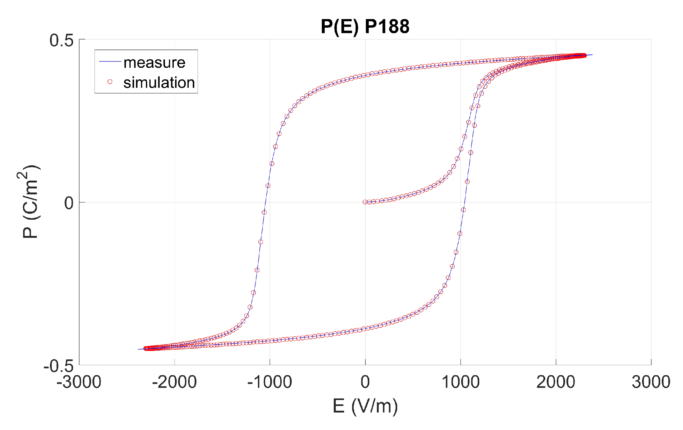
2. Hysteresis Model of Ferroelectrics Transducers

Common semipassive and active surrounding ambient mechanical vibration harvesters work under a weak level of mechanical excitation. Most of the time, those levels are assumed to be sufficiently low to consider the relation between excitation and induced quantities as linear [21]. To improve system efficiency and increase the amount of harvested energy, switching techniques like the SSHI energy extractor described in this introduction intentionally enhance the excitation amplitude. In terms of simulation, the main drawback of this excitation amplitude is that it increases linear material relations, which makes it no longer suitable, and it has to be replaced by more sophisticated models, including saturation, hysteresis, and frequency dependence. Such approaches are necessary to achieve an agreement between numerical and experiment results. On the basis of experiment observations, an accurate piezo-ceramic hysteresis model was established suitable for large frequency bandwidths and for providing precise simulation results, whatever the shape and the nature of the excitation (triangular or sinusoidal, electrical, or mechanical) [22,23,24,25]. The present hysteresis model is constituted of two contributions: quasistatic (frequency-independent) and dynamic contribution.

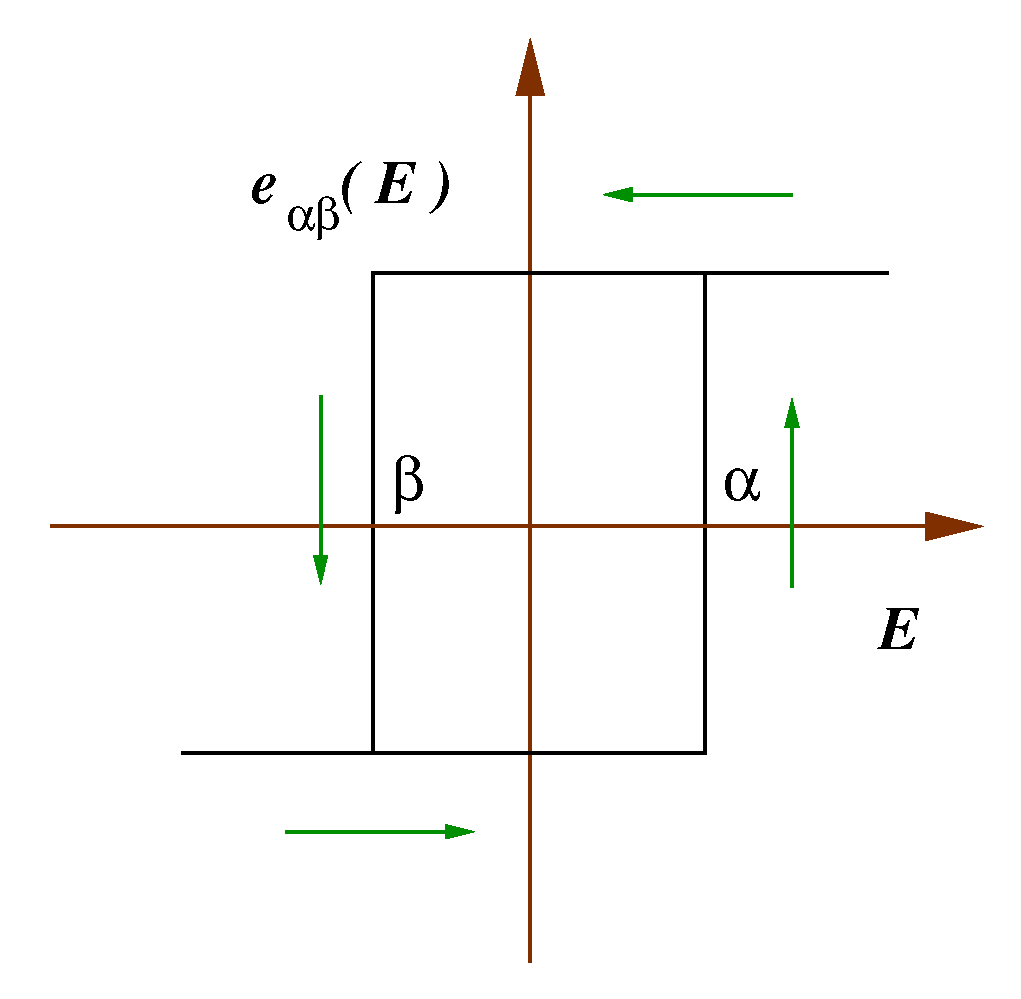
2.1. Quasistatic Contribution

The usual looplike hysteresis is observed when plotting unforced polarization P versus electrical field E [20] in the low-frequency limit ( f 1 Hz) and fairly high excitation amplitudes. Such a result defines the quasistatic hysteresis state. Various simulation approaches of quasistatic hysteresis behavior can be found in the scientific literature. Among all, the Preisach model [26] exhibited the interesting property of being easily reversible, namely, it was possible to interchange E and P as inputs and outputs of the quasistatic hysteresis model. The Preisach model was first developed to describe the hysteresis phenomenon in ferromagnetic materials [27]. More recently, it has also been successfully employed for ferroelectric hysteresis consideration [28,29]. In the case of dielectric hysteresis, the Preisach model assumes that material polarization is determined by the contribution of a set of elementary hysteresis loops having a distribution function over the Preisach triangle.
Instead of a simple linear relation between electrical field E and polarization P,
P = ε 0 χ E ,
where ε 0 is the vacuum permittivity constant, χ = ε r 1 is dielectric material susceptibility, ε r is relative static permittivity. We then have more general integral relation
P = f s t a t i c ( E ) = P s a t + + μ ( E α , E β ) e α , β ( E ) d E α d E β ,
which, after normalization, leads to:
+ + μ ( E α , E β ) d E α d E β = 1 ,
where E α and E β are branching fields for a single hysteron with probability distribution μ ( E α , E β ) and e α , β is a single decreasing or increasing hysteron line (see Figure 2), while P s a t is saturation polarization (see Figure 3).
A precise and accurate simulation of the hysteretic behavior of the ferroelectric material requires to accurately determine the Preisach distribution function. For this, we needed experiment results. We basically had two options to calculate corresponding distribution function μ ( E α , E β ) . The first assumes that μ ( E α , E β ) can be expressed by using a mathematical analytical expression (Lorentzian, Gaussian). Variations from one material to another come from the parameters of this analytical function. On the other hand, the second option discretizes μ into a set of values ( E α , E β ) determined later by comparison between simulation tests and experiment results. In this study, we aimed for the second option as it was expected to have higher-accuracy results. Among all available methods, two important techniques were comprehensively tested for the estimation and acquisition of the discretized distribution function. The first is based on the centered-cycle approach [30], while the other, the Biorci–Pescetti method [31,32] is based on the first magnetization (polarization) curve.
After several simulation tests, we observed that both techniques provided accurate simulation results. However, a larger amount of experiment data was required by the first technique, while correct behavior could be reached with a lower distribution size with the second technique. Consequently, smaller distribution means simpler and reduced memory management. Therefore, in this specific study, where calculation accuracy was required, and access to many experiment results for the implementation of our model was granted, the centered-cycle technique was a good option. However, once we apply the Biorci–Pescetti method [31] to obtain proper probability distribution (Figure 2), then its corresponding hysteresis (Figure 3) in the correct shape could simultaneously be obtained. Figure 3 shows a comparison of simulated/measured major dielectric hysteresis cycle P ( E ) while the branching point probability μ ( E α , E β ) is shown in Figure 4. The experiment loop was obtained using the experiment setup described in [33]. Because of space limitation, this comparison is the only one displayed here, but a large number of further numerical simulation validations on the same material can be found elsewhere [32,33,34,35,36]. All these already published results confirm the validation of the piezoceramic ferroelectric behavior as demonstrated in the simulation results in this work.

2.2. Dynamic Contribution

As soon as we increased excitation field E frequency and exceeded the quasistatic limit (≈10 mHz for the P188 ceramics used in this study), the piezoceramic exhibited hysteresis loops strongly resembling a frequency-dependent hysteresis loop. A second contribution was required to consider this dependence in the simulation. The dynamic hysteresis effect is usually introduced in the literature as the product of an equivalent dissipative operator ρ to the instantaneous time derivative of polarization d P / d t . Consequently, ρ d P / d t then acts as an equivalent electric field. As illustrated in [20], this dynamic consideration provides correct simulation results on very narrow frequency bandwidth. In the case of SSHI systems, we deal with large frequency variations; to obtain correct simulation results, large frequency bandwidth models are required. By defining parameter ρ by using comparison simulation/results under low-frequency levels, integer-order time derivative d P / d t consideration led to overestimation of the hysteresis area curve as frequency increased. To overcome this problem, we replaced the first-order time derivation of the polarization by fractional derivation [33,34,35,36]. This mathematical operator gives an additional degree of freedom and allows to differently balance low- and high-frequency variations. After adding fractional terms in our simulation, the model equation became:
ρ d n P ( t ) d t n = E ( t ) f s t a t i c 1 ( P ) ,
where n < 1 denotes a fractional order. In this paper, we used n = 0.56 .

2.3. Mechanical-Stress Consideration
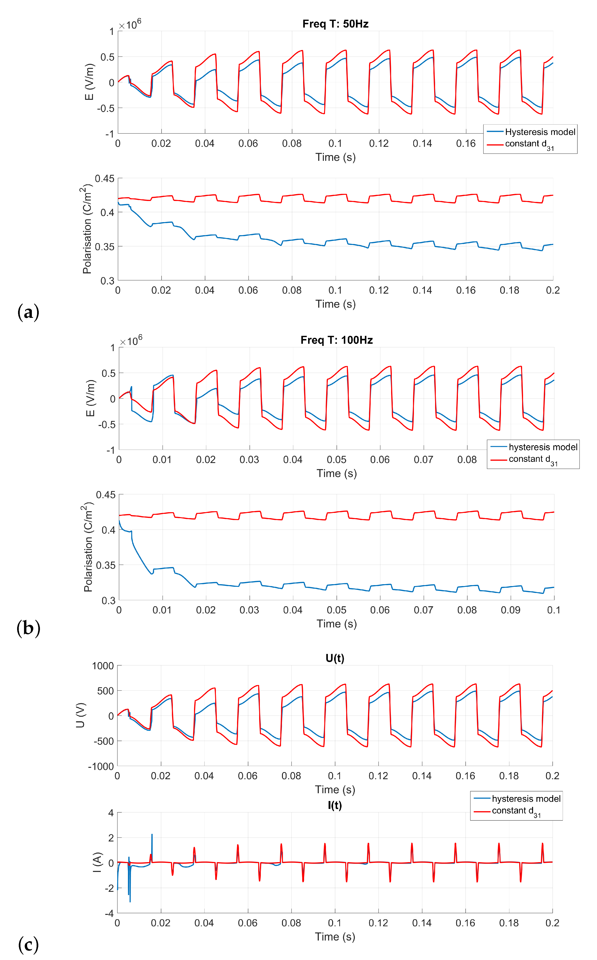
Under external mechanical compressive stress, piezoelectric polarization is affected by the coupling term. In our case, we involved the piezoelectric layer that was subjected to elongation and contraction. The simplified equations are:
ρ d n P i ( t ) d t n = E ( t ) + α T ( t ) P i ( t ) f s t a t i c 1 ( P i ) ,
where T ( t ) is imposed harmonically changing mechanical stress
T ( t ) = T 0 sin ( ω t ) ,
and α is a coupling constant.
Note that this model has a general form but does not include the effects of instantaneous switching at the maximum stress instants. This is discussed in the next section.

3. SSHI Model

Analysis of focused models of intelligent structures has gained considerable attention since the 1970s. In particular, the formulation of the lumped model, presented by Alika and Hughes [37] on the basis of the variational principle, has been widely referenced. Our model includes a piezoelectric element and has a degree of freedom for simplicity. As a matter of fact, a mechanical model only relies on one degree of freedom and gives a good description of vibrating structure behavior near its resonant frequencies. In this study, the objective was to check the influence of the material law on the efficiency of the SSHI system [15,16]. As a first step and to simplify the model, we assumed that the piezoceramic was subjected to harmonically changing mechanical stress. The maximum of the mechanical stress was then easily detectable. The model circuit possesses piezoelement equivalent capacity C:
C = ε 0 χ A / l ,
where A is a surface of electrodes and l is a distance between them, inductance L or load resistivity R l . In our simplified model, we assumed the electrodes’ geometrical values as constants. Depending on the switching option (see Figure 5), the output voltage on the electrodes was governed to the voltage V output on the inductor or load resistor R L and capacitor C L , respectively.
When the stress reached maximum value T = T m a x , the first option was used, internal resistivity R was very small, and output voltage on the electrodes was the following:
V = V ( T m a x ) exp ( t / τ ) cos ( ω 0 t ) ,
where τ = 1 / R L / C denotes a relaxation ratio of the RLC circuit, and ω 0 = 1 / L C is a natural frequency of the LC circuit. In this time, almost no power output was generated on load resistance R L . After the fast recharging of electrodes (in the time interval δ t ) the load resistor R L is switched starting the voltage output of the order V ( T m a x ) exp ( δ t / τ ) . At this point the mechanical stress was changing working to further increase output voltage and, consequently, power output (see Figure 6). Note that mechanical strain S is linked to polarization P thanks to the following relation:
S = α P 2 .
Using the above equations (Equations (5)–(9)), we performed simulations of the dynamical response. Results are presented in Figure 6, Figure 7 and Figure 8, while system parameters are outlined in Table 1. Two distinct phases can be observed on the electric-field time chronogram, displayed in Figure 6.
The first phase is where the switch was opened and where the electric-field variations were linked to mechanical-stress excitation (Equation (5)). The scaling relation between electric field and mechanical stress E = α T P was then used.
The second phase was where the switch was closed and where the electric-field variations were linearly linked to the parallel capacitance voltage drop expressed in Equation (8). For the polarization field chronogram, Equation (5) is solved considering both electric field E and α T P as excitation sources.
The voltage chronogram (time series) was obtained from the electric field and thanks to linear relation E = U / l (Figure 6c). The current chronogram was obtained using a time derivation of the polarization. The time variations of the electric field, mechanical stress, and polarization state gave access to time-dependent permittivity and by linearity to the capacitance. The piezoelectric capacitance time chronogram was obtained by solving capacitance equation C ( t ) = ε 0 ε r ( t ) A / l , where A and l, sample surface and thickness, respectively, were assumed to be constant. The electrostatic energy time chronogram was obtained thanks to the equation of electrostatic energy being equal to C ( t ) V 2 ( t ) / 2 , where V ( t ) is the time-dependent capacitance voltage. Figure 8a,b were obtained by plotting P ( t ) as a function of E ( t ) . Figure 7 and Figure 8 outline the early overshoot of the piezocapacitance and electrostatic energy due to the transient phase that took place between the poling phase and the harvesting-beam setup steady state. Figure 8b shows the minor P ( E ) hysteresis cycle obtained once this transient phase was over. On this figure, both the switching-on and -off period are clearly distinguishable.
The presented results compare the simulation of the system with nonlinear (hysteretic) material characteristics (Equations (2)–(5)) to the linear model results (Equation (1)). We started the simulation from the first polarization curve (see Figure 8).
Figure 6a,b shows electrical field E and polarization P for two imposed frequencies of stress T: f = 50 and 100 Hz. Clearly, the influence of the hysteretic response (blue line) according to the linear model (red line) was stronger for a higher frequency. This is better visible on the polarization time series. The difference can be explained by additional damping in the hysteretic model. Further information is shown in Figure 6c, where voltage U and current I (in the case of f = 50 Hz) are presented. These are related to the quantities on the piezoelectric electrodes and not the load resistor. In Figure 7, we additionally show capacity variations and electrostatic energy in piezoelectric electrodes. Obviously, the energy was smaller in the model with hysteresis. In the linear case, electrode capacity was constant, while in hysteretic mode it was dependent on dynamic susceptibility
χ = P ( t ) ε 0 E ( t )
Finally, the first polarization with the working stationary point are plotted in Figure 8a, and the resulting steady-state hysteresis is shown in Figure 8b. Comparing it to quasistatic hysteresis (Figure 3), it was distorted, as a variable electrical field is not an external driving parameter, but it is related to the switching mechanism. However, minor cycle hysteresis was still noticeable and could alter harvested energy estimations. In this article, we focused on the simulation of a mechanical vibration energy harvester. The first experiment validation we opted for came from the dielectric piezoceramic behavior, as commented in Section 2.1. The huge differences observed between simulation results using constant d31 and the hysteresis model led to the conclusion that correct simulation results could only be obtained from the real nonlinear behavior of the material. To validate our simulations, we considered that the shape of the piezoceramic voltage dropped sufficiently close to the experiment shape (Figure 1) with regard to real-time variations (Figure 6c). Furthermore, simulation results on the basis of the proposed SSHI hysteretic model and experiment qualitative verifications on the time history of piezoceramic voltage U and electrical current I are presented in Figure 9. For this purpose, we used fairly small mechanical excitation amplitude on the piezoelectric beam and rescaled the electrical response by a fitted constant. Their good agreement was remarkable.

4. Conclusions

For more than 20 years now, synchronized-switching devices have allowed huge improvements in the level of harvested energy from semipassive and active surrounding ambient mechanical vibration harvesters. Unfortunately, some limitations remain, and dielectric losses through piezoelements is one of them. One drawback of the switching methods comes from increasing the piezoceramic parallel capacitance voltage drop that creates large electri-field variations, and consequently increases the dielectric level of losses and creates transient phases. A linear consideration of the dielectric behavior leads to huge errors in the evaluation of the whole system efficiency. In this article, simulations were proposed to compare dielectric-linear and hysteretic behavior. Significant differences on hysteresis-loop P ( E ) working point could be observed. For our assumed conditions, hysteretic behavior reduced efficiency in energy conversion and, consequently, harvested energy by about 15% (see Figure 6a); however, the inclination of the polarization curve stayed on the same angle. Simultaneously, due to additional damping by material hysteresis, the frequency band was slightly broader, contributing to a frequency broadband effect. The results could be even more important if one considers the polymer piezoelectric foil where electrical dipoles are more susceptible to polarization. Finally, we focused on a piezoelectric-beam-type harvester, but similar relations and techniques could be used to simulate every kind of electromechanical piezoelectric conversion.

Author Contributions

All authors have contributed to this work. G.L. initiated the studies, B.D. performed the calculations, and all the authors (B.D., B.G., and G.L.) analyzed the results and prepared the manuscript.

Funding

This publication was supported by the program of the Ministry of Science and Higher Education in Poland under project DIALOG 0019/DLG/2019/10 for 2019–2021.

Conflicts of Interest

The authors declare no conflict of interest.

References

  1. Mitcheson, P.D.; Yeatman, E.M.; Rao, G.K.; Holmes, A.S.; Green, T.C. Energy harvesting from human and machine motion for wireless electronic devices. Proc. IEEE 2008, 96, 1457–1486. [Google Scholar] [CrossRef]
  2. Litak, G.; Manoach, E. Dynamics of composite nonlinear systems and materials for engineering applications and energy harvesting—The role of nonlinear dynamics and complexity in new developments. Eur. Phys. J. Spec. Top. 2013, 222, 1479–1482. [Google Scholar] [CrossRef]
  3. Litak, G.; Manoach, E.; Halvorsen, E. Nonlinear and multiscale dynamics of smart materials in energy harvesting. Eur. Phys. J.-Spec. Top. 2015, 224, 2671–2673. [Google Scholar] [CrossRef]
  4. Harne, R.L.; Wang, K.W. A review of the recent research on vibration energy harvesting via bistable systems. Smart Mat. Struct. 2013, 22, 023001. [Google Scholar] [CrossRef]
  5. Pellegrini, S.P.; Tolou, N.; Schenk, M.; Herder, J.L. Bistable vibration energy harvesters: A review. J. Intell. Mater. Syst. Struct. 2013, 24, 1303–1312. [Google Scholar] [CrossRef]
  6. Twiefel, J.; Westermann, H. Survey on broadband techniques for vibration energy harvesting. J. Intell. Mater. Syst. Struct. 2013, 24, 1291–1302. [Google Scholar] [CrossRef]
  7. Daqaq, M.F.; Masana, R.; Erturk, A.; Quinn, D.D. On the role of nonlinearities in vibratory energy harvesting: A critical review and discussion. Appl. Mech. Rev. 2014, 66, 040801. [Google Scholar] [CrossRef]
  8. Huguet, T.; Badel, A.; Druet, O.; Lallart, M. Drastic bandwidth enhancement of bistable energy harvesters: Study of subharmonic behaviors and their stability robustness. Appl. Energy 2018, 226, 607–617. [Google Scholar] [CrossRef]
  9. Huang, D.; Zhou, S.; Litak, G. Theoretical analysis of multi-stable energy harvesters with high order stiffness terms. Commun. Nonlinear Sci. Numer. Simul. 2019, 69, 270–286. [Google Scholar] [CrossRef]
  10. Lallart, M.; Lefeuvre, E.; Richard, C.; Guyomar, D. Self-powered circuit for broadband, multimodal piezoelectric vibration control. Sens. Actuator A 2008, 143, 377–382. [Google Scholar] [CrossRef]
  11. Guyomar, D.; Richard, C.; Mohammadi, S. Damping behavior of semi-passive vibration control using shunted piezoelectric materials. J. Intell. Mater. Syst. Struct. 2008, 19, 977–985. [Google Scholar] [CrossRef]
  12. Kelley, C.R.; Kauffman, J.L. Adaptive synchronized switch damping on an inductor: A self-tuning switching law. Smart Mater. Struct. 2017, 26, 035032. [Google Scholar] [CrossRef]
  13. Zouari, M.; Naifar, S.; Bouattour, G.; Derbel, N.; Kanoun, O. Energy management based on fractional open circuit and P-SSHI techniques for piezoelectric energy harvesting. tm-Technisches Messen 2019, 86, 14–24. [Google Scholar] [CrossRef]
  14. Qureshi, E.M.; Shen, X.; Chen, J. Vibration control laws via shunted piezoelectric transducers: A review. Int. J. Aeronaut. Space Sci. 2014, 15, 1–19. [Google Scholar] [CrossRef]
  15. Badel, A.; Guyomar, D.; Lefeuvre, E.; Richard, C. Piezoelectric Energy Harvesting using a Synchronized Switch Technique. J. Intell. Mater. Syst. Struct. 2006, 17, 831–839. [Google Scholar] [CrossRef]
  16. Badel, A.; Benayad, A.; Lefeuvre, E.; Lebrun, L.; Richard, C.; Guyomar, D. Single Crystals and Nonlinear Process for Outstanding Vibration Powered Electrical Generators. IEEE Trans. Ultrason. Ferroelect. Freq. Contr. 2006, 53, 673–684. [Google Scholar] [CrossRef]
  17. Lefeuvre, E.; Sebald, G.; Guyomar, D.; Lallart, M.; Richard, C. Materials, structures and power interfaces for efficient piezoelectric energy harvesting. J. Electroceram 2009, 22, 171–179. [Google Scholar] [CrossRef]
  18. Guyomar, D.; Badel, A.; Lefeuvre, E.; Richard, C. Toward Energy Harvesting Using Active Materials and Conversion Improvement by Nonlinear Processing. IEEE Trans. Ultrason. Ferroelect. Freq. Contr. 2005, 52, 584–595. [Google Scholar] [CrossRef]
  19. Lefeuvre, E.; Badel, A.; Richard, C.; Petit, L.; Guyomar, D.A. Comparison between several vibration-powered piezoelectric generators for standalone systems. Sens. Actuator A Phys. 2006, 126, 405–416. [Google Scholar] [CrossRef]
  20. Ducharne, B.; Guyomar, D.; Sebald, G. Low frequency modelling of hysteresis behavior and dielectric permittivity in ferroelectric ceramics under electric field. J. Phys. D Appl. Phys. 2007, 40, 551–555. [Google Scholar] [CrossRef]
  21. Priya, S. Advances in energy harvesting using low profile piezoelectric transducers. J. Electroceram. 2007, 19, 167–184. [Google Scholar] [CrossRef]
  22. Zhang, B.; Ducharne, B.; Guyomar, D.; Sebald, G. Energy harvesting based on piezoelectric Ericsson cycles in a piezoceramic material. Eur. Phys. J.-Spec. Top. 2013, 222, 1733–1743. [Google Scholar] [CrossRef]
  23. Zhang, B.; Ducharne, B.; Gupta, B.; Sebald, G.; Guyomar, D.; Gao, J. Experimental sea wave energy extractor based on Piezoelectric Ericsson cycles. J. Int. Mater. Syst. Struct. 2017, 26, 1102–1112. [Google Scholar] [CrossRef]
  24. Zhang, B.; Ducharne, B.; Sebald, G.; Guyomar, D. Characterization of fractional order for high-frequency bandwidth model of dielectric ferroelectrics. J. Intell. Mater. Syst. Struct. 2016, 27, 437–443. [Google Scholar] [CrossRef]
  25. Wang, D.; Wang, L.; Melnik, R. Vibration energy harvesting based on stress-induced polarization switching: A phase field approach. Smart Mater. Stuct. 2017, 26, 065022. [Google Scholar] [CrossRef]
  26. Mayergoyz, I.D. Mathematical Models of Hysteresis and Their Applications, 1st ed.; Elsevier: Amsterdam, The Netherlands, 2003. [Google Scholar]
  27. Preisach, F. Über die magnetische Nachwirkung. Zeitschrift Physik. 1935, 94, 277–302. [Google Scholar] [CrossRef]
  28. Sutor, A.; Rupitsch, S.J.; Lerch, R. A Preisach based hysteresis model for magnetic and ferroelectric hysteresis. Appl. Phys. A 2010, 100, 425–430. [Google Scholar] [CrossRef]
  29. Bernard, Y.; Maalej, H.; Lebrun, L.; Ducharne, B. Preisach modelling of ferroelectric behavior. Int. J. Appl. Electr. Mech. 2007, 25, 729–733. [Google Scholar]
  30. Bernard, Y.; Mendes, E.; Ren, Z. Determination of the distribution function of Preisach’s model using centred cycles. COMPEL-Int. J. Comput. Math. Electr. Electron. Eng. 2000, 19, 997–1006. [Google Scholar] [CrossRef]
  31. Biorci, G.; Pescetti, D. Some Remarks on Hysteresis. J. Appl. Phys. 1966, 37, 425–427. [Google Scholar] [CrossRef]
  32. Zhang, B.; Gupta, B.; Ducharne, B.; Sebald, G.; Uchimoto, T. Preisach’s model extended with dynamic fractional derivation contribution. IEEE Trans. Magn. 2017, 54, 6100204. [Google Scholar] [CrossRef]
  33. Guyomar, D.; Ducharne, B.; Sebald, G. High frequency bandwidth polarization and strain control using a fractional derivative inverse model. Smart Mater. Struct. 2010, 19, 045010. [Google Scholar] [CrossRef]
  34. Ducharne, B.; Zhang, B.; Guyomar, D.; Sebald, G. Fractional derivative operators for modeling piezo ceramic polarization behaviors under dynamic mechanical stress excitation. Sens. Actuator A-Phys. 2013, 189, 74–79. [Google Scholar] [CrossRef]
  35. Guyomar, D.; Ducharne, B.; Sebald, G. The use of fractional derivation in modeling ferroelectric dynamic hysteresis behavior over large frequency bandwidth. J. Appl. Phys. 2010, 107, 114108. [Google Scholar] [CrossRef]
  36. Guyomar, D.; Ducharne, B.; Sebald, G.; Audigier, D. Fractional derivative operator for modeling dynamical polarization behaviour as a function of frequency and electric field amplitude. IEEE Trans. Ultrason. Ferroelectr. Freq. Control 2009, 56, 437–443. [Google Scholar] [CrossRef] [PubMed]
  37. Alik, H.; Hughes, T.J.R. Finite element method for piezoelectric vibration. Int. J. Numer. Methods Eng. 1970, 2, 151–157. [Google Scholar] [CrossRef]
Figure 1. (a) Synchronized Switch Damping on an Inductor (SSDI) device; (b) voltage V and displacement U waveforms; (c) transducer voltage inversion zoom.
Energies 12 04466 g001
Figure 2. Single hysteron operator: increasing and decreasing functions e α , β ( E ) .
Energies 12 04466 g002
Figure 3. Hysteresis with first polarization using Biorci–Pescetti method [31].
Energies 12 04466 g003
Figure 4. Branching-point probability μ ( E α , E β ) distribution ( E α and E β ). Extreme value of P is saturation polarization P s a t .
Energies 12 04466 g004
Figure 5. (a) Schematics of piezoelectric beam and electrical circuit with switchers. (b) Active part.
Energies 12 04466 g005
Figure 6. Time series starting from first polarization by a high electrical field and a stationary solution with mechanical excitation and simultaneous switching circuit for: electrical field E on the electrodes and polarization P of a piezoelectric material or two different excitation frequencies (a) 50 Hz and (b) 100 Hz. (c) Voltage U and corresponding current I versus time during excitation. In the first phase (500 s), the sample was polarized and then harmonically excited (as illustrated). In the simulation, we assumed no time delay, but it could also be introduced without any influence on the results.
Energies 12 04466 g006
Figure 7. (a) Time variation of piezoelement-equivalent capacity. (b) Time variations of electrostatic energy ( C V 2 / 2 ) through piezoelement-equivalent capacity.
Energies 12 04466 g007
Figure 8. (Color online) (a) First polarization curve P versus applied electrical field E. Time variations of current and voltage along piezoelement. (b) Hysteresis curve (P versus E of dynamical model). These results are based on time series presented in previous figures (Figure 6a,c and Figure 7) for f = 50 Hz.
Energies 12 04466 g008
Figure 9. Comparison simulation/measurement for time variation of piezoceramic voltage U and electrical current I.
Energies 12 04466 g009
Table 1. Simulation parameters used in equation set (Equations (5)–(9)).
Parameter α n ρ Al T 0 ω ω 0 τ L
Value0.030.5620,000 4 × 10 4 0.001 2 × 10 7 2 π f 20 π f 0.1160
UnitsV N 1 C 1 m 3 -V S n C 1 m 2 n 1 m 2 mmN m 2 rad s 1 rad s 1 sH

