Comprehensive Harmonic Responsibility Calculation Based on Different Weighting Methods

Abstract

Dividing the responsibility of harmonics between customer and utility sides is necessary to improve the objectivity, rationality, and scientificalness of power measurement and power quality evaluation. On the basis of expert experience and customer needs and considering the background harmonic fluctuation, this study proposes two reasonable conditions to evaluate harmonic responsibility. At the same time, the reference index of harmonic responsibility calculation and the problem of different frequency harmonics are considered in the comprehensive calculation. On the basis of the IEEE Std. 1459–2010 power theory, the index set of harmonic responsibility is established, and several common subjective and objective weighting methods are used to weigh each index. On the basis of optimization theory, an optimization model is established by constructing a Lagrange function in finding the condition extremum to unify the subjective and objective information. Finally, the calculation method is verified by a Norton equivalent model, and the harmonic responsibility of each index is calculated by the harmonic current vector method; thus, calculating the actual impedance of customer and utility sides is unnecessary, making the calculation simple and effective. Results of the comparative analysis show that the comprehensive evaluation method of harmonic responsibility with the combinatorial weighting method can not only meet the different needs of different groups for harmonic indicators but also reflect the background harmonic fluctuations sensitively. In this manner, the subjective and objective information are unified, and the shortcomings of a single weighting method are overcome. Hence, the evaluation results are accurate, practical, and reasonable.

1. Introduction

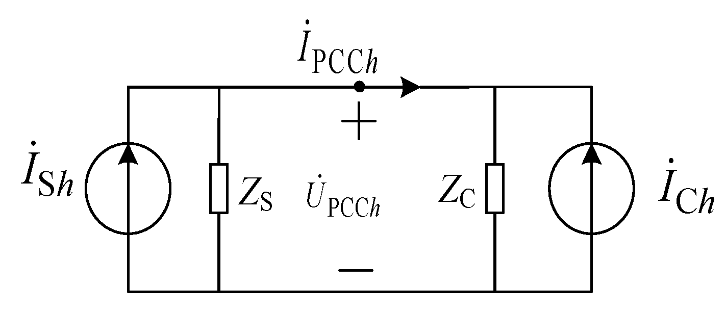
With the rapid development of power electronics and nonlinear loads, harmonics in power systems have gradually become serious, thereby attracting increasing scientific research attention. First, the harmonics have been analyzed in detail [1]. With the development of the subject, researchers have proposed several positioning methods of the main harmonic source [2,3,4]; however, these methods only locate the main harmonic source, but they cannot calculate the harmonic responsibility of each harmonic source quantitatively. Reference [5] first proposed the calculation of harmonic responsibility in 2002; the model of calculation of harmonic responsibility is shown in Figure 1. With the development of this topic, many researchers begin to focus on modeling approach of utility side and customer side [6,7,8], calculation method of parameters of modeling [9], and so on. Among them, the calculation method of impedance of utility side has been research focus in recent years [10,11,12,13]. Compared with different models, such as constant current source, Norton equivalent model, and the admittance matrix model, results showed that the Norton equivalent model is the most cost-effective [14]. Harmonic current vector method can be utilized to calculate harmonic responsibility without any information of the actual impedance of customer side and utility side; it provides a method which is easily applied to calculate parameters of customer side and utility side [15].

According to calculation model of harmonic responsibility, which is based on the Norton equivalent model shown in Figure 1, the calculation of parameters of the utility side and customer side is obviously very important, thus proposing fluctuation method, binary linear regression, and so on. Compared with harmonic current vector method, these methods show some practical deficiencies.

The traditional calculation method of harmonic responsibility mainly focuses on the contributions of the harmonic current and the harmonic voltage at the point of common coupling (PCC). Therefore, Reference [16] proposed the index of harmonic current and harmonic voltage based on superposition theory. Some researchers have explored the comprehensive evaluation of harmonic responsibility and obtained some results in the evaluation method. In Reference [17], the PCC point current was divided into distorted and non-distorted currents, which were used as the basis for the division of harmonic current at the utility and customer sides, but only applicable to the case where the customer side was pure resistance load. In Reference [18], the load current was divided into two parts, namely, nonlinear and linear currents, which were used as the basis for the division of the harmonic responsibility of the customer side. The quantitative evaluation index was provided; however, this method was unsuitable for the condition of utility side distortion. In Reference [19], the principles of harmonic current index and harmonic voltage index were analyzed in detail, and the two principles were relatively different; thus, the calculation results of harmonic responsibility were also different. Reference [20] indicated that the fluctuation of harmonic voltage and current is large in the case of background harmonic fluctuation. Moreover, the calculation results of existing methods may have large deviation, and they cannot reflect the variation characteristics of harmonic voltage and current nor consider the effect of background harmonic fluctuation. In addition, the traditional index based on the superposition theory was used to calculate the harmonic responsibility under the specific harmonic frequency, which lacks further research on the combination of different frequencies. Therefore, the relevant staff often is often confused when selecting the harmonic responsibility calculation index due to the lack of unity [19]. Currently, Emanuel proposed the latest power theory standard IEEE Std. 1459–2010, which defines different power physical quantities under different conditions [21] and provides a standard for relevant workers to measure physical quantities under harmonic conditions. Similar to the calculations of harmonic responsibility, the comprehensive evaluation of power quality also needs to combine different indicators [22,23,24,25], which provide enlightenment for comprehensive harmonic responsibility calculation.

For the responsibility evaluation, determining the weight that corresponds to the evaluation index is important. The change of the weight value has a direct effect on the rationality of the comprehensive evaluation and thus on the comprehensive evaluation of harmonic responsibility. In view of the aforementioned problems, this study proposes the idea of the comprehensive harmonic responsibility calculation, which can evaluate the harmonic responsibility of each of the harmonic sources more comprehensively and accurately compared to the previously published work. On the basis of the actual situation, this study presents two reasonable judgment conditions for the comprehensive calculation method of the harmonic responsibility based on different weighting methods, establishes the indicator set of harmonic responsibility based on IEEE Std. 1459–2010 power theory, and selects several commonly used subjective and objective weighting methods. At the same time, on the basis of optimization theory, the subjective and objective weighting methods are combined as the combinatorial weighting method (CWM) for assigning the evaluation indicators.

The remainder of this paper is organized as follows. Section 2 presents the process of comprehensive harmonic responsibility calculation. Section 3 introduces and analyzes different methods of empowerment. Section 4 establishes an example of harmonic responsibility calculation using Matlab/Simpower system. The simulation results verify the practicability of the different weighting methods in the comprehensive harmonic responsibility calculation. Section 5 presents the results of the CWM on the basis of the proposed two reasonable judgment conditions.

2. Comprehensive Harmonic Responsibility Calculation

In practice, different harmonic responsibility indicators have different effects on power systems and users. For example, voltage distortion has a considerable effect on power systems; thus, the customer side should take greater responsibility for distorted voltage. The injected harmonic current also has a more serious effect on the customer side. Thus, the utility side should take greater responsibility for the distorted current, and the opposite applies to the customer side. In practice, the fifth harmonic problem is likely to be caused by the system, whereas the third harmonic problem is likely to be caused by the user. Thus, the customer side should bear less responsibility for the fifth harmonic and greater responsibility for the third harmonic. By contrast, under the background harmonic fluctuation condition, the fluctuation of harmonic voltage and current on the utility and customer sides are relatively large, and the harmonic parameters in the actual power grid change with time. Therefore, evaluation results should reflect the changes of data sensitively. In sum up, the following conditions should be fully considered for the reasonable division of harmonic liability:

Condition 1: The evaluation results should meet the different needs of customer side and utility side for harmonic indicators.

Condition 2: The evaluation results should reflect the change of background harmonic sensitively.

Therefore, the comprehensive calculation steps of harmonic responsibility are as follows.

First, the index set of harmonic responsibility calculation is established based on IEEE Std. 1459–2010. In IEEE Std. 1459–2010, the apparent power is decomposed in detail, and the equation can be expressed as follows:

$$\begin{array}{cc}\hfill S^2& ={(UI)}^2=(U_1^2+U_{\mathrm{H}}^2)(I_1^2+I_{\mathrm{H}}^2)\hfill \\ & ={(U_1{I}_1)}^2+{(U_1{I}_{\mathrm{H}})}^2+{(U_{\mathrm{H}}{I}_1)}^2+{(U_{\mathrm{H}}{I}_{\mathrm{H}})}^2\hfill \\ & =S_1^2+D_I^2+D_{\mathrm{U}}^2+S_{\mathrm{H}}^2=S_1^2+S_{\mathrm{N}}^2\hfill \end{array}$$

(1)

$$D_{\mathrm{I}}=U_1{I}_{\mathrm{H}}=U_1\sqrt{{\displaystyle \sum _{h=2}^{\infty }{I}_h^2}}$$

(2)

$$D_{\mathrm{U}}=U_{\mathrm{H}}{I}_1=I_1\sqrt{{\displaystyle \sum _{h=2}^{\infty }{U}_h^2}}$$

(3)

$$S_{\mathrm{H}}=U_{\mathrm{H}}{I}_{\mathrm{H}}=\sqrt{{\displaystyle \sum _{h=2}^{\infty }{U}_h^2}·{\displaystyle \sum _{h=2}^{\infty }{I}_h^2}}$$

(4)

where U_H and I_H are the RMS values of harmonic voltage and harmonic current, respectively; U₁ and I₁ are the RMS values of fundamental voltage and fundamental current, respectively; S₁ is the fundamental apparent power; D_U is the voltage distortion power; D_I is the current distortion power; S_H is the harmonic apparent power; S_N is the nonfundamental apparent power; and U_h and I_h are the RMS values of harmonic voltage and harmonic current under hth harmonic, respectively.

Equation (1) indicates that IEEE Std. 1450–2010 separates the fundamental and harmonic parts. Nonfundamental apparent power S_N represents all physical quantities that are relevant to harmonics.

According to the decomposition of apparent power in IEEE Std. 1459–2010, the index set of harmonic responsibility calculation is established in Figure 2.

The physical quantities corresponding to each index can be expressed as follows:

$$D_{\mathrm{I}h}=U_1{I}_h$$

(5)

$$D_{\mathrm{V}h}=U_h{I}_1$$

(6)

$$S_{\mathrm{H}h}=U_h{I}_h$$

(7)

where D_Vh is the voltage distortion power under hth harmonic; D_Ih is the current distortion power under hth harmonic; S_Hh is the harmonic apparent power under hth harmonic, respectively. Because the content of S_H in S_N is the smallest in practice, only the product of harmonic voltage and current at the same frequency is considered.

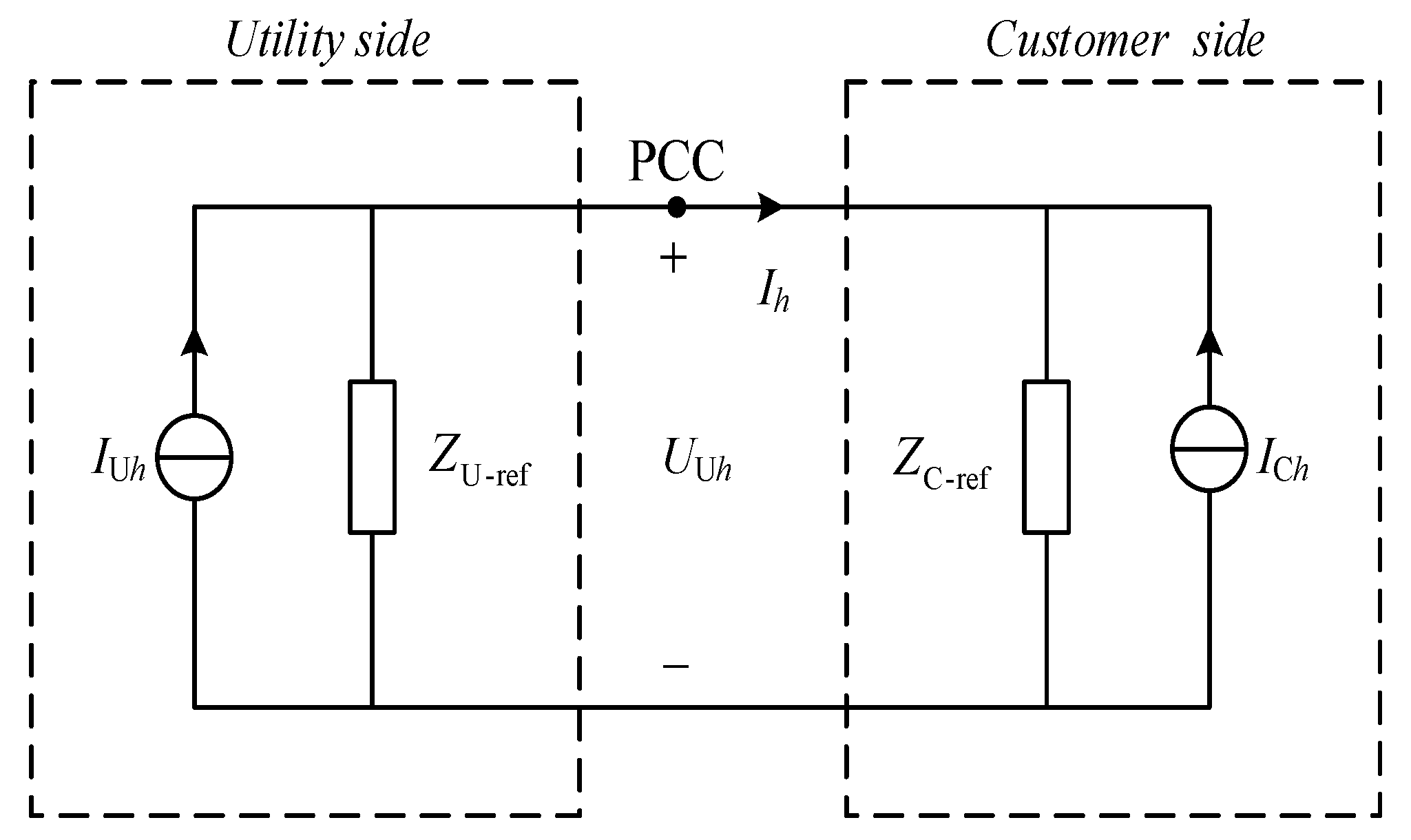
Second, the calculation model of harmonic contribution is established. On the basis of the model of harmonic responsibility in Figure 1, the calculation model of the harmonic contribution of the utility and customer sides based on superposition theory on the PCC point can be established in Figure 3.

On the basis of the index set established in Figure 2 and the calculation model of the harmonic contribution of the utility and customer sides, the harmonic responsibility based on each index in the index set of utility/customer side is calculated, respectively.

Finally, the comprehensive harmonic responsibility is calculated based on different weighting methods. The weight $W_i$ of each index in the index set is calculated by different weighting methods, which will be introduced in detail in Section 3. Then, the comprehensive harmonic responsibility of the utility/customer side is calculated by combining the calculation results of the harmonic responsibility and the weight of each index, respectively, as shown as follows:

$$R_{\mathrm{u}}^{*}={\displaystyle \sum _{i=1}^n{W}_{i-\mathrm{u}}{R}_{i-\mathrm{u}}}$$

(8)

$$R_{\mathrm{c}}^{*}={\displaystyle \sum _{i=1}^n{W}_{i-\mathrm{c}}{R}_{i-\mathrm{c}}}$$

(9)

$$R_{\mathrm{u}}=\frac{R_{\mathrm{u}}^{*}}{R_{\mathrm{u}}^{*}+R_{\mathrm{c}}^{*}}$$

(10)

$$R_{\mathrm{c}}=\frac{R_{\mathrm{c}}^{*}}{R_{\mathrm{u}}^{*}+R_{\mathrm{c}}^{*}}$$

(11)

where $R_{i-\mathrm{u}}^{}$ and $R_{i-\mathrm{c}}^{}$ are the harmonic responsibilities based on each index of the utility and customer sides, respectively; $W_{i-\mathrm{u}}^{}$ and $W_{i-\mathrm{c}}^{}$ are the weights of each index of the utility and customer sides, respectively; $R_{\mathrm{u}}^{\ast }$ and $R_{\mathrm{c}}^{*}$ are the initial values of the comprehensive harmonic responsibility of the utility and customer sides, respectively; $R_{\mathrm{u}}^{}$ and $R_{\mathrm{c}}^{}$ are the comprehensive harmonic responsibility of the utility and customer sides, respectively; and n is the number of index i.

3. Different Weighting Methods of Comprehensive Harmonic Responsibility Calculation

Equations (8)–(11) indicate that the calculation of the weight of each index $W_i$ is an important step and has a deep influence on the result of the comprehensive harmonic responsibility calculation of the utility and customer sides. Therefore, several common weighting methods are introduced as follows.

3.1. Analytic Hierarchy Process (AHP))

AHP was proposed by American mathematician T.L. Saaty. It is used to calculate the subjective weight of each index in the index set [26,27,28]. This method can avoid consistency checking using the calculation process of a judgment matrix to reduce the complexity of calculation. However, this approach is difficult to be convinced due to its small quantitative data and several qualitative components. The calculation steps are as follows.

First, the judgment matrix is calculated. At the same layer of indexes, indexes are placed in order; two adjacent indexes are compared with each other. The element $b_{ij}^{}$ of the judgment matrix B represents the importance of index i to index j.

Table 1. Value of $b_{ij}^{}$ of judgment matrix B.

$\mathbf{Value}\mathbf{of}{\mathit{b}}_{\mathit{i}\mathit{j}}^{}$	Verbal Judgments of Preferences
1	Equally preferred
1.2	Moderately preferred
1.4	Strongly preferred
1.6	Very strongly preferred
1.8	Extremely preferred

lists the values of element $b_{ij}^{}$.

Judgment matrix B can be expressed as:

$$B=\left[\begin{array}{ccccc}1& b_{12}& b_{12}{b}_{23}& \dots & b_{12}{b}_{23}{b}_{34}\dots b_{(n-1)n}\\ \raisebox{1ex}{$1$}\!\left/ \!\raisebox{-1ex}{$b_{12}$}\right.& 1& b_{23}& \dots & b_{23}{b}_{34}\dots b_{(n-1)n}\\ \raisebox{1ex}{$1$}\!\left/ \!\raisebox{-1ex}{$b_{12}{b}_{23}$}\right.& \raisebox{1ex}{$1$}\!\left/ \!\raisebox{-1ex}{$b_{23}$}\right.& 1& \dots & b_{34}\dots b_{(n-1)n}\\ \dots & \dots & \dots & \dots & \dots \\ \raisebox{1ex}{$1$}\!\left/ \!\raisebox{-1ex}{$b_{12}{b}_{23}{b}_{34}\dots b_{(n-1)n}$}\right.& \raisebox{1ex}{$1$}\!\left/ \!\raisebox{-1ex}{$b_{23}{b}_{34}\dots b_{(n-1)n}$}\right.& \raisebox{1ex}{$1$}\!\left/ \!\raisebox{-1ex}{$b_{34}\dots b_{(n-1)n}$}\right.& \dots & 1\end{array}\right]$$

(12)

On the basis of the calculation of judgment matrix B, the subjective weight $W_{i-\mathrm{AHP}}$ of index i can be expressed as:

$$W_{i-\mathrm{AHP}}=\frac{1}{{\displaystyle \sum _{i=1}^n\frac{1}{b_{ij}}}}$$

(13)

where b_ij is the element at row i and column j of B, and n is the number of indexes.

3.2. Expert Consultation Method (ECM)

ECM is a type of market approach simulation that uses experts’ knowledge, experience, and analytical judgment to verify a reference index. ECM is used to calculate the subjective weight of each index in the index set. This method is simple and practicable and is convenient in application. However, it is greatly influenced by subjective factors that may affect the accuracy of the conclusion [29]. Four steps are involved in ECM.

First, the original weight of each index in the index set is calculated. On the basis of personal experience and understanding, some experts are invited to evaluate the weight of each index; these weights are called original weights. The sum of the original weights given by the same expert should be equal to 1:

$${\displaystyle \sum _{i=1}^n{o}_{li}}=1$$

(14)

where $o_{li}$ represents the original weight of index i given by expert l.

Second, the average weight of index i is calculated:

$${\overline{o}}_i=\frac{{\displaystyle \sum _{l=1}^d{o}_{li}}}{d}$$

(15)

where ${\overline{o}}_i$ represents the average weight of index i, and d represents the total number of experts.

Third, the offset $o_{li}^{*}$ of weight of index i is calculated:

$$o_{li}^{*}=\left|o_{li}-{\overline{o}}_i\right|$$

(16)

Fourth, the modified weight $W_{i-\mathrm{ECM}}$ of index i is calculated by ${\overline{o}}_{li}^{*}$ and $u_i$, as shown as follows:

$${\overline{o}}_{li}^{*}=\frac{\underset{i}{{\displaystyle \max }} o_{li}^{*}-o_{li}^{*}}{\underset{i}{\max } o_{li}^{*}-\underset{i}{\min } o_{li}^{*}}$$

(17)

$$u_i=\frac{{\displaystyle \sum _{l=1}^d({\overline{o}}_{li}^{*}{o}_{li})}}{{\displaystyle \sum _{l=1}^d{\overline{o}}_{li}^{*}}}$$

(18)

$$W_{i-\mathrm{ECM}}=\frac{u_i}{{\displaystyle \sum _{i=1}^n{u}_i}}$$

(19)

3.3. Entropy Weighting Method (EWM)

EWM was proposed by Clausius. It is used to calculate the objective weight of each index in the index set. The entropy value is obtained by calculation; the larger it is, the higher the disorder of the event will be, and thus, the smaller the contribution to the final evaluation result will be [30,31]. By contrast, the higher the order of the event is, the greater the contribution to the final evaluation result will be. EWM complies with objective rules and has strict mathematical significance. However, it is not necessarily in line with actual needs because the subjective intentions of policy makers are often neglected. The calculation steps are as follows. First, an evaluation of each index in the index set can be used to obtain fuzzy mapping. On the basis of the definition of fuzzy transformation, fuzzy mapping can determine a fuzzy relation F called fuzzy evaluation matrix.

$$\mathit{F}=\left[\begin{array}{cccc}{f}_{11}& f_{12}& \cdots & f_{1m}\\ f_{21}& f_{22}& \cdots & f_{2m}\\ ⋮& ⋮& \cdots & ⋮\\ f_{n1}& f_{n2}& \cdots & f_{nm}\end{array}\right]$$

(20)

where f_nm represents the fuzzy relation between index n and rank m.

On the basis of the calculation of judgment matrix F, $H_i$, expressed as Equation (18), is the entropy of index expressed as Equation (19), which is the sum of the entropy of each index.

$$H_i=-\frac{1}{\ln m}{\displaystyle \sum _{j=1}^m(f_{ij}\ln f_{ij})}$$

(21)

$$E={\displaystyle \sum _{i=1}^n{H}_i}$$

(22)

where m is the number of ranks of each index.

The objective weight $W_{i-\mathrm{EWM}}$ of index i can be expressed as:

$$W_{i-\mathrm{EWM}}=\frac{1}{n-E}(1-H_i)$$

(23)

3.4. Variation Coefficient Method (VCM)

VCM is an objective weighting method, and it is similar to the entropy weighting method. If the variation of index i is large, then different ranks of index i can be distinguished well, and the weight should then be large [32,33]. This method can eliminate the influence of dimension and measurement scale, but it lacks attention to the practical significance of indexes. Four steps are used in the application of VCM.

On the basis of fuzzy evaluation matrix F, which is expressed as Equation (14), the first step is to calculate the average value of index i:

$${\overline{f}}_i=\frac{1}{m}{\displaystyle \sum _{j=1}^m{f}_{ij}}$$

(24)

The second step is to calculate the standard deviation of index i:

$${\varsigma }_i=\sqrt{\frac{1}{m}{\displaystyle \sum _{j=1}^m{\left(f_{ij}-{\overline{f}}_i\right)}^2}}$$

(25)

The third step is to calculate the value of variation of index i:

$$v_i=\frac{{\varsigma }_i}{{\overline{f}}_i}$$

(26)

The fourth step is to calculate the weight $W_{i-\mathrm{VCM}}$ of index i:

$$W_{i-\mathrm{VCM}}=\frac{v_i}{{\displaystyle \sum _{i=1}^n{v}_i}}$$

(27)

3.5. Combinational Weighting Method (CWM)

The basic idea of CWM is to combine the weights that are calculated by the single weighting method mentioned above, considering subjective preferences of policy makers and the objectivity of index data, thereby achieving the unity of subjective and objective information. Common combination methods include addition combinations and multiplication combinations. The addition combination method is extremely inflexible to distinguish the good and bad information from the subjective and objective weight information. The multiplication combination method will cause a “multiplication effect”, which is only applicable to the case of having many indicators and uniform weight distributions. Therefore, on the basis of the idea that the deviation between the weights of the CWM and the single weighting method is as small as possible, the following model is established:

$$\{\begin{array}{l}\min F\left(\omega \right)=\frac{1}{2}{\displaystyle \sum _{i=1}^n(\alpha ({(({\omega }_i-W_{i-\mathrm{AHP}})R_i)}^2+{(({\omega }_i-W_{i-\mathrm{EWM}})R_i)}^2)}\\ +(1-\alpha )({(({\omega }_i-W_{i-\mathrm{ECM}})R_i)}^2+{(({\omega }_i-W_{i-\mathrm{VCM}})R_i)}^2)\\ \mathrm{S}.\mathrm{T}.{\displaystyle \sum _{i=1}^n{\omega }_i=1,{\omega }_i\ge 0}\end{array}$$

(28)

where ${\omega }_i$ is the weight of index i after combination, $R$ is the evaluation matrix established on the harmonic responsibility of each index, n is the number of index i, 0 ˂ α ˂ 1 is the coefficient of subjective preference, and 0 ˂ 1 − α ˂ 1 is the coefficient of objective preference. By setting the value of α, the analyst’s preference for subjective and objective weights can be adjusted flexibly.

The Lagrange function is established to solve the model as follows:

$$\begin{array}{l}L\left({\omega }_i,\lambda \right)=\frac{1}{2}{\displaystyle \sum _{i=1}^n(\alpha ({(({\omega }_i-W_{i-\mathrm{AHP}})R_i)}^2+{(({\omega }_i-W_{i-\mathrm{EWM}})R_i)}^2)}\\ +(1-\alpha )({(({\omega }_i-W_{i-\mathrm{ECM}})R_i)}^2+{(({\omega }_i-W_{i-\mathrm{VCM}})R_i)}^2)\\ +2\lambda \left({\displaystyle \sum _{i=1}^n{\omega }_i-1}\right)\end{array}$$

(29)

On the basis of the necessary conditions for the existence of extremes, the following is set:

$$\{\begin{array}{l}\frac{\partial L}{\partial {\omega }_i}=\alpha ({(({\omega }_i-W_{i-\mathrm{AHP}})R_i)}^2+{(({\omega }_i-W_{i-\mathrm{EWM}})R_i)}^2)\\ {\displaystyle +(1-\alpha )({(({\omega }_i-W_{i-\mathrm{ECM}})R_i)}^2+{(({\omega }_i-W_{i-\mathrm{VCM}})R_i)}^2)+2\lambda =0}\\ \frac{\partial L}{\partial \lambda }={\displaystyle \sum _{i=1}^n{\omega }_i}-1=0\end{array},$$

(30)

which can be simplified as:

$$\begin{array}{l}\{\begin{array}{l}\frac{1}{2}{\omega }_i{R}_i^2+\lambda =\frac{1}{2}\left(\alpha \left(W_{i-\mathrm{AHP}}+W_{i-\mathrm{EWM}}\right)+\left(1-\alpha \right)\left(W_{i-\mathrm{ECM}}+W_{i-\mathrm{VCM}}\right)\right)R_i^2\\ {\displaystyle \sum _{i=1}^n{\omega }_i}=1\end{array}\end{array}$$

(31)

and represented as matrix as:

$$\left[\begin{array}{cc}A& e\\ e^{\mathrm{T}}& 0\end{array}\right]\left[\begin{array}{c}W\\ \lambda \end{array}\right]=\left[\begin{array}{c}B\\ 1\end{array}\right]$$

(32)

where:

$$A_{n\times n}=\mathrm{diag}\left[R_1^2,R_2^2,\dots ,R_n^2\right]$$

(33)

$$B_{n\times 1}={\left[b_1,b_2,\dots ,b_n\right]}^{\mathrm{T}}$$

(34)

$$b_i=\left(\alpha \left(W_{i-\mathrm{AHP}}+W_{i-\mathrm{EWM}}\right)+\left(1-\alpha \right)\left(W_{i-\mathrm{ECM}}+W_{i-\mathrm{VCM}}\right)\right)z_i^2$$

(35)

$$e_{n\times 1}={\left(1,1,\dots ,1\right)}^{\mathrm{T}}$$

(36)

$$W_{n\times 1}={\left({\omega }_1,{\omega }_2,\dots ,{\omega }_n\right)}^{\mathrm{T}}$$

(37)

By solving the matrix equation (Equation (29)), the following results can be obtained:

$$W_{n\times 1}=A^{-1}\left[B+\frac{1-e^{\mathrm{T}}{A}^{-1}B}{e^{\mathrm{T}}{A}^{-1}e}e\right]$$

(38)

$$W_{i-\mathrm{CWM}}={\omega }_i$$

(39)

4. Example and Simulation Analysis

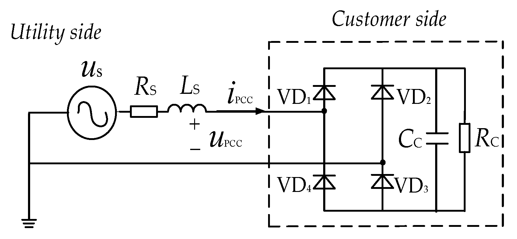
As an example, the simulation model is established in Figure 4. The utility side contains a certain amount of background harmonics, whereas the customer side is an uncontrollable rectifier circuit. The parameters of the simulation model are set in

Table 2. Parameters of the simulation model.

Parameter	${\mathit{u}}_{\mathbf{S}1}$	${\mathit{u}}_{\mathbf{S}3}$	${\mathit{u}}_{\mathbf{S}5}$	${\mathit{R}}_{\mathbf{S}}$	${\mathit{L}}_{\mathbf{S}}$	${\mathit{R}}_{\mathbf{C}}$	${\mathit{C}}_{\mathbf{C}}$
Value	$220\angle 0^{°}\mathrm{V}$	$4\angle {150}^{°}\mathrm{V}$	$2\angle {160}^{°}\mathrm{V}$	2 Ω	2 mH	2 Ω	1200 $\mathsf{\mu }\mathrm{F}$

.

Comprehensively considering the third and fifth harmonics, the index set is established based on Figure 2. Then, on the basis of the measurement data on the PCC point, the parameters of the Norton equivalent model of the utility and customer sides are obtained by the improved impedance method [15], and the reference impedance of the utility side is selected as the actual impedance in the simulation.

$$Z_{\mathrm{C}-\mathrm{ref}}=\frac{U_{\mathrm{PCC}1}{}^2}{P_1}=\frac{U_{\mathrm{PCC}1}}{I_{\mathrm{PCC}1}\cos {\alpha }_1}=1.7348\mathsf{\Omega }$$

(40)

$${\dot{I}}_{\mathrm{C}3}=\frac{{\dot{U}}_{\mathrm{PCC}3}}{Z_{\mathrm{C}-\mathrm{ref}}}-{\dot{I}}_{\mathrm{PCC}3}=3.1963\angle 131.7127°\mathrm{A}$$

(41)

$${\dot{I}}_{\mathrm{C}5}=\frac{{\dot{U}}_{\mathrm{PCC}5}}{Z_{\mathrm{C}-\mathrm{ref}}}-{\dot{I}}_{\mathrm{PCC}5}=2.3373\angle 129.2146°\mathrm{A}$$

(42)

$$Z_{\mathrm{U}3-\mathrm{ref}}=R_{\mathrm{S}}+\mathrm{j}{\omega }_3{L}_{\mathrm{S}}=2+1.885\mathrm{i}\mathsf{\Omega }=2.748\angle 43.30°\mathsf{\Omega }$$

(43)

$$Z_{\mathrm{U}5-\mathrm{ref}}=R_{\mathrm{S}}+\mathrm{j}{\omega }_5{L}_{\mathrm{S}}=2+3.142\mathrm{i}\mathsf{\Omega }=3.725\angle 57.518°\mathsf{\Omega }$$

(44)

$${\dot{I}}_{\mathrm{U}3}=\frac{{\dot{U}}_{\mathrm{PCC}3}}{Z_{\mathrm{U}3-\mathrm{ref}}}+{\dot{I}}_{\mathrm{PCC}3}=2.0746\angle 149.3470°\mathrm{A}$$

(45)

$${\dot{I}}_{\mathrm{U}5}=\frac{{\dot{U}}_{\mathrm{PCC}3}}{Z_{\mathrm{U}5-\mathrm{ref}}}+{\dot{I}}_{\mathrm{PCC}5}=0.7083\angle 115.8667°\mathrm{A}$$

(46)

where $U_{\mathrm{PCC}h}$ and $I_{\mathrm{PCC}h}$ represent the RMS value of voltage and current under the hth harmonic, respectively; α₁ is the phase angle difference between the fundamental voltage and fundamental current on PCC; $Z_{\mathrm{C}-\mathrm{ref}}$ represents the reference impedance of the customer side; $Z_{\mathrm{U}h-\mathrm{ref}}$ denotes the reference impedance of the utility side under the hth harmonic; and ${\dot{I}}_{\mathrm{C}h}$ and ${\dot{I}}_{\mathrm{U}h}$ are the harmonic current sources under the hth harmonic of the customer and utility sides, respectively.

The harmonic responsibility of different indexes in the index set can be calculated on the basis of the calculation of utility/customer side parameters. Take the 3rd harmonic as an example, and the responsibility based on index 1, 3, 5 can be calculated as follows:

$$R_{\mathrm{DV}3-\mathrm{u}}=\frac{U_{\mathrm{u}-3\mathrm{rd}}}{U_{\mathrm{u}-3\mathrm{rd}}+U_{\mathrm{c}-3\mathrm{rd}}},R_{\mathrm{DV}3-\mathrm{c}}=\frac{U_{\mathrm{c}-3\mathrm{rd}}}{U_{\mathrm{u}-3\mathrm{rd}}+U_{\mathrm{c}-3\mathrm{rd}}}$$

(47)

$$R_{\mathrm{DI}3-\mathrm{u}}=\frac{I_{\mathrm{u}-3\mathrm{rd}}}{I_{\mathrm{u}-3\mathrm{rd}}+I_{\mathrm{c}-3\mathrm{rd}}},R_{\mathrm{DI}3-\mathrm{c}}=\frac{I_{\mathrm{c}-3\mathrm{rd}}}{I_{\mathrm{u}-3\mathrm{rd}}+I_{\mathrm{c}-3\mathrm{rd}}}$$

(48)

$$R_{\mathrm{SH}3-\mathrm{u}}=\frac{U_{\mathrm{u}-3\mathrm{rd}}{I}_{\mathrm{u}-3\mathrm{rd}}}{U_{\mathrm{u}-3\mathrm{rd}}{I}_{\mathrm{u}-3\mathrm{rd}}+U_{\mathrm{c}-3\mathrm{rd}}{I}_{\mathrm{c}-3\mathrm{rd}}},R_{\mathrm{SH}3-\mathrm{c}}=\frac{U_{\mathrm{c}-3\mathrm{rd}}{I}_{\mathrm{c}-3\mathrm{rd}}}{U_{\mathrm{u}-3\mathrm{rd}}{I}_{\mathrm{u}-3\mathrm{rd}}+U_{\mathrm{c}-3\mathrm{rd}}{I}_{\mathrm{c}-3\mathrm{rd}}}$$

(49)

Table 3. Calculation results of harmonic responsibility based on different indexes.

Index	1 (DV3)	2 (DV5)	3 (DI3)	4 (DI5)	5 (SH3)	6 (SH5)
Utility Side (%)	39.36	23.25	48.10	36.36	37.56	14.76
Customer Side (%)	60.64	76.75	51.90	63.64	62.44	85.24

shows the calculation results.

The harmonic responsibilities based on different indexes in the index set should be obtained together to calculate the harmonic responsibility of the utility/customer side. Thus, the calculation of each index weight is important.

In practice, the harmonic parameters change with time under the background harmonic fluctuation; thus, harmonic responsibility calculation should be considered under the background harmonic fluctuation. The cases selected for this study are shown in

Table 4. Cases of harmonic responsibility calculation.

Case	Harmonic Responsibility Calculation
1	Background harmonic random fluctuates
2	Background harmonic under indexes 1 and 5 fluctuate violently

to enable the behavioral analysis of the methods.

4.1. Case 1

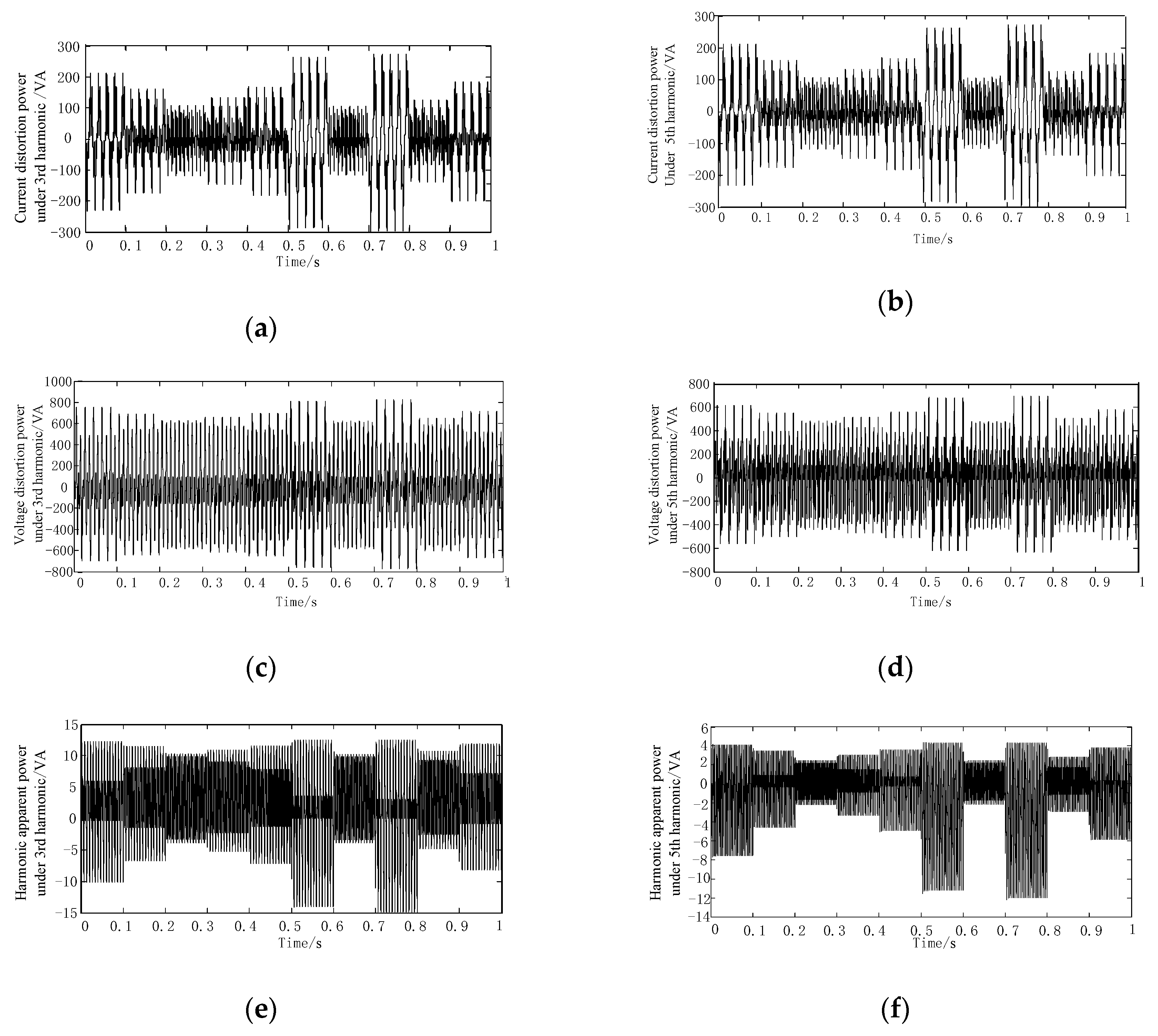
In this case, the random number model is used to simulate the fluctuation of the customer side, and it can generate a uniformly distributed random number with a variance of 3 and a mean of 0, which is shown in the Appendix A. On the basis of the maximum and minimum corresponding physical quantities of each index in the index set, each index is divided into four levels on average within observation time, which is assumed to be 1 s. On the basis of the above level classification standard, the time statistics of the four power indexes that appear in the corresponding levels can be obtained in

Table 5. Time statistics of different physical quantities.

i	Physical Quantity	Time Statistics (s)
		Level 1	Level 2	Level 3	Level 4
1	DV3	0.5015	0.1973	0.2241	0.0773
2	DV5	0.5089	0.2988	0.1570	0.0355
3	DI3	0.5598	0.3062	0.1063	0.0278
4	DI5	0.6492	0.2402	0.0826	0.0281
5	SH3	0.4227	0.2757	0.2294	0.0723
6	SH5	0.7284	0.1921	0.0422	0.0375

.

On the basis of Table 5, the fuzzy evaluation matrix ${\mathit{T}}_{\mathrm{case}1}$ can be obtained as:

$${\mathit{T}}_{\mathrm{case}1}=\left[\begin{array}{cccc}0.5015& 0.1973& 0.2241& 0.0773\\ 0.5089& 0.2988& 0.1570& 0.0355\\ 0.5598& 0.3062& 0.1063& 0.0278\\ 0.6492& 0.2402& 0.0826& 0.0281\\ 0.4227& 0.2757& 0.2294& 0.0723\\ 0.7284& 0.1921& 0.0422& 0.0375\end{array}\right]$$

(50)

AHP method: The index set is established based on Figure 2 for the application of the AHP method. Referring to the experts’ experience and users’ requirements, the power supply company and the relevant power users are involved in the division of harmonic responsibility simultaneously. Indexes i are in the following order from 1 to 6 as follows: D_V3, D_V5, D_I3, D_I5, S_H3, and S_H5. The following are also set: t₁₂ = 1.6, t₂₃ = 1.8, t₃₄ = 1.8, t₄₅ = 1.8, and t₅₆ = 1.2. On the basis of Equation (12), judgment matrix B, which depends on the decision maker, is expressed as follows:

$$\mathit{B}=\left[\begin{array}{cccccc}1& 1.6& 2.88& 5.184& 9.3312& 11.1974\\ \raisebox{1ex}{$1$}\!\left/ \!\raisebox{-1ex}{$1.6$}\right.& 1& 1.8& 3.24& 5.832& 6.9984\\ \raisebox{1ex}{$1$}\!\left/ \!\raisebox{-1ex}{$2.88$}\right.& \raisebox{1ex}{$1$}\!\left/ \!\raisebox{-1ex}{$1.8$}\right.& 1& 1.8& 3.24& 3.888\\ \raisebox{1ex}{$1$}\!\left/ \!\raisebox{-1ex}{$5.184$}\right.& \raisebox{1ex}{$1$}\!\left/ \!\raisebox{-1ex}{$3.24$}\right.& \raisebox{1ex}{$1$}\!\left/ \!\raisebox{-1ex}{$1.8$}\right.& 1& 1.8& 2.16\\ \raisebox{1ex}{$1$}\!\left/ \!\raisebox{-1ex}{$9.3312$}\right.& \raisebox{1ex}{$1$}\!\left/ \!\raisebox{-1ex}{$5.832$}\right.& \raisebox{1ex}{$1$}\!\left/ \!\raisebox{-1ex}{$3.24$}\right.& \raisebox{1ex}{$1$}\!\left/ \!\raisebox{-1ex}{$1.8$}\right.& 1& 1.2\\ \raisebox{1ex}{$1$}\!\left/ \!\raisebox{-1ex}{$11.1974$}\right.& \raisebox{1ex}{$1$}\!\left/ \!\raisebox{-1ex}{$6.9984$}\right.& \raisebox{1ex}{$1$}\!\left/ \!\raisebox{-1ex}{$3.888$}\right.& \raisebox{1ex}{$1$}\!\left/ \!\raisebox{-1ex}{$2.16$}\right.& \raisebox{1ex}{$1$}\!\left/ \!\raisebox{-1ex}{$1.2$}\right.& 1\end{array}\right]$$

(51)

Then, based on Equations (51) and (13), the weight $W_{i-\mathrm{c}-\mathrm{AHPcase}1}$ of each index of the customer side is shown in

Table 6. Weight of each index based on different subjective weighting methods.

Weight			1 (DV3)	2 (DV5)	3 (DI3)	4 (DI5)	5 (SH3)	6 (SH5)
AHP	Customer Side	Case 1	0.4234	0.2647	0.1470	0.0817	0.0454	0.0378
		Case 2	0.4234	0.2647	0.1470	0.0817	0.0454	0.0378
	Utility Side	Case 1	0.0884	0.1592	0.2547	0.4076	0.0409	0.0491
		Case 2	0.0884	0.1592	0.2547	0.4076	0.0409	0.0491
ECM	Customer Side	Case 1	0.3758	0.2618	0.1553	0.1035	0.0518	0.0518
		Case 2	0.3758	0.2618	0.1553	0.1035	0.0518	0.0518
	Utility Side	Case 1	0.1122	0.1543	0.2572	0.3734	0.0514	0.0514
		Case 2	0.1122	0.1543	0.2572	0.3734	0.0514	0.0514

.

ECM: For the use of ECM, six experts are invited to evaluate the weight of each index, and indexes are in the following evaluation order: D_V3, D_V5, D_I3, D_I5, S_H3, and S_H5. Then, the original weight matrix O can be assumed as:

$$\mathit{O}=\left[\begin{array}{cccccc}0.35& 0.25& 0.15& 0.10& 0.10& 0.05\\ 0.35& 0.30& 0.15& 0.10& 0.05& 0.05\\ 0.40& 0.20& 0.15& 0.15& 0.05& 0.05\\ 0.45& 0.15& 0.20& 0.10& 0.05& 0.05\\ 0.35& 0.30& 0.15& 0.05& 0.10& 0.05\\ 0.25& 0.25& 0.20& 0.10& 0.10& 0.10\end{array}\right]$$

(52)

Then, on the basis of Equations (52) and (14)–(19), the weight $W_{i-\mathrm{c}-\mathrm{ECMcase}1}$ of each index of the customer side is shown in Table 6.

EWM: On the basis of the fuzzy evaluation matrix, ${\mathit{T}}_{\mathrm{case}1}$ is obtained as Equation (50). When using the EWM based on Equations (21)–(23), the weight $W_{i-\mathrm{c}-\mathrm{EWMcase}1}$ of each index of the customer side is shown in

Table 7. Weight of each index based on different objective weighting methods.

Weight			1 (DV3)	2 (DV5)	3 (DI3)	4 (DI5)	5 (SH3)	6 (SH5)
EWM	Case 1	Customer Side	0.0935	0.1363	0.1808	0.2286	0.0670	0.2911
		Utility Side	0.0935	0.1363	0.1808	0.2286	0.0670	0.2911
	Case 2	Customer Side	0.3119	0.0613	0.0813	0.1028	0.3119	0.1309
		Utility Side	0.3119	0.0613	0.0813	0.1028	0.3119	0.1309
VCM	Case 1	Customer Side	0.1307	0.1482	0.1731	0.2047	0.1052	0.2382
		Utility Side	0.1307	0.1482	0.1731	0.2047	0.1052	0.2382
	Case 2	Customer Side	0.2441	0.0993	0.1159	0.1371	0.2441	0.1596
		Utility Side	0.2441	0.0993	0.1159	0.1371	0.2441	0.1596

.

VCM: On the basis of the fuzzy evaluation matrix, ${\mathit{T}}_{\mathrm{case}1}$ is obtained as Equation (50). On the basis of Equations (24)–(27), the weight $W_{i-\mathrm{c}-\mathrm{VCMcase}1}$ of each index of the customer side is shown in Table 7.

CWM: When using the CWM based on Equations (28)–(39) on the basis of the weight calculated above (α = 0.5 indicates that subjective and objective weights are of equal importance), the weight $W_{i-\mathrm{c}-\mathrm{CWMcase}1}$ of each index of customer side is shown in

Table 8. Weight of each index based on CWM.

Weight			1 (DV3)	2 (DV5)	3 (DI3)	4 (DI5)	5 (SH3)	6 (SH5)
CWM	Customer Side	Case 1	0.2602	0.2046	0.1577	0.1542	0.0681	0.1551
		Case 2	0.3396	0.1728	0.1219	0.1062	0.1641	0.0954
	Utility Side	Case 1	0.1062	0.1495	0.2164	0.3036	0.0668	0.1575
		Case 2	0.1891	0.1185	0.1773	0.2552	0.1621	0.0978

.

The weight calculation procedure of each index on the utility side is the same as that on the customer side and will thus not be repeated here. Then, the weight of each index for Case 1 on the utility side based on the subjective, objective, and combinational weighting methods is shown in Table 6, Table 7 and Table 8, respectively. The comprehensive harmonic responsibility of the utility/customer side for Case 1 can be obtained on the basis of Equations (8)–(11), as shown in

Table 9. Calculation result of harmonic responsibility based on different weighting methods.

Harmonic Responsibility		AHP	ECM	EWM	VCM	CWM
Case 1	Customer Side (%)	63.99	64.01	69.23	68.18	66.33
	Utility Side (%)	36.01	35.99	30.77	31.82	33.67
Case 2	Customer Side (%)	63.99	64.01	65.01	66.00	64.75
	Utility Side (%)	36.01	35.99	34.99	34.00	35.25

.

4.2. Case 2

On the basis of Case 1, assuming that background harmonics under indexes 1 and 5 fluctuate violently, the time for them to be in the fourth stage is 1 s and that in other stages is 0 s during the entire measurement period. Then, the fuzzy evaluation matrix ${\mathit{T}}_{\mathrm{case}2}$ is given as follows:

$${\mathit{T}}_{\mathrm{case}2}=\left[\begin{array}{cccc}0& 0& 0& 1\\ 0.5089& 0.2988& 0.1570& 0.0355\\ 0.5598& 0.3062& 0.1063& 0.0278\\ 0.6492& 0.2402& 0.0826& 0.0281\\ 0& 0& 0& 1\\ 0.7284& 0.1921& 0.0422& 0.0375\end{array}\right]$$

(53)

AHP and ECM: These methods are subjective weighting methods that are qualitatively weighted. They are weighted based on the importance of each index to the power grid and customer. Thus, the calculation results of Case 2 will not change because only the background harmonic situation changes. Taking the customer side as an example, that is $W_{i-\mathrm{c}-\mathrm{AHPcase}2}=W_{i-\mathrm{c}-\mathrm{AHPcase}1}$, $W_{i-\mathrm{c}-\mathrm{ECMcase}2}=W_{i-\mathrm{c}-\mathrm{ECMcase}1}$.

EWM and VCM: This approach is based on ${\mathit{T}}_{\mathrm{case}2}$, in which the fuzzy evaluation matrix is shown in Equation (53). Then, on the basis of Equations (20)–(27), the weights of each index on the customer side by the entropy weight method ($W_{i-\mathrm{c}-\mathrm{EWMcase}2}$) and the coefficient of variation method ($W_{i-\mathrm{c}-\mathrm{VCMcase}2}$) are shown in Table 7.

CWM: By using the CWM based on Equations (28)–(39) on the basis of the weight calculated above, the weight ($W_{i-\mathrm{c}-\mathrm{CWMcase}2}$) of each index of the customer side is shown in Table 8.

The weight calculation procedure of each index on the utility side is the same as that on the customer side and will thus not be repeated here. Then, the weight of each index of Case 2 on the utility side based on the subjective, objective, and combinational weighting methods is shown in Table 6, Table 7 and Table 8, respectively. On the basis of Equations (8)–(11), the comprehensive harmonic responsibility of the utility and customer sides for Case 1 can be obtained, as shown in Table 9.

4.3. Comparisons of Calculation Results Based on Different Weighting Methods

On the basis of the subjective weighting method, the weight of each index on the customer and utility sides are calculated, as shown in Table 6.

AHP and ECM: Table 6 shows that the weights of the customer and utility sides based on AHP and ECM are different. The distribution trend is consistent with the actual effect of harmonics on the customer and the utility sides. Moreover, given that these subjective weighting methods are based on the experts’ comprehensive evaluation of the effect of each index in various aspects from their level of understanding and experiment, the subjective weighting method meets Condition 1. However, in Table 6, the weight of each index corresponding to Case 2 based on these methods has not changed any more than that of Case 1. That is to say, the weights obtained by these methods are not sensitive to the change of harmonics in a power system; thus, it cannot meet Condition 2.

On the basis of the objective weighting method, the weight of each index on the customer and utility sides are calculated, as shown in Table 7.

EWM and VCM: Table 7 shows that among the objective weights based on EWM and VCM, the weights corresponding to indexes 1 and 5 account for a large proportion in Case 2, which is obviously different from Case 1. This condition is consistent with the presupposition. Thus, the objective weighting method meets Condition 2. However, the weight distribution of the customer side is exactly the same as that of the utility side, which is not consistent with the actual demand of the customer and utility sides for each index. Therefore, the entropy weight method and the coefficient of variation method cannot reflect the different demands of power systems and users for harmonic indexes. Therefore, Condition 1 cannot be satisfied.

On the basis of CWM, the weight of each index on the customer and utility sides are calculated, as shown in Table 8.

CWM: The weight in Table 8 shows that the weights distribution based on CWM in Cases 1 and 2 are consistent with the different influences of each index on the customer and utility sides in the actual situation. Thus, the rationality Condition 1 is satisfied. Furthermore, in Case 2, when indexes 1 and 5 change considerably, the corresponding weights change remarkably compared with Case 1. The change trend is consistent with the present situation. Therefore, the CWM can satisfy Conditions 1 and 2.

The analysis of comprehensive harmonic responsibility is obtained by different weighting methods.

On the basis of the weights obtained by different weighting methods, combined with Equations (5)–(8), the harmonic responsibility of the customer/utility side are calculated, as shown in Table 9.

Taking Case 1 as an example, Table 9 shows that in the single weighting method, little difference of harmonic responsibility value is obtained by a similar weighting method. By contrast, the difference obtained by the different weighting methods is large. The calculation results obtained by the CWM are between them. Therefore, selecting the appropriate weighting method is of considerable importance for the accuracy of harmonic responsibility calculation.

The harmonic responsibility of Cases 1 and 2 in Table 9 show that the calculation results based on the subjective weighting method are identical, whereas the harmonic responsibility of Case 2 based on the objective and the CWM is obviously different from that of Case 1. Therefore, neglecting the fluctuation of background harmonic may result in a certain amount of error.

The evaluation results are not sensitive to the changes of index parameters, and the evaluation results are greatly affected by subjective factors. Although objective weighting can reflect this change sensitively, it cannot reflect the different demands of different power users for harmonic indexes. It may give a large weight for some indexes that are considered unimportant by researchers. The CWM proposed in this study combines these subjective and objective weighting methods. It can reflect the subjective will, meet the different needs of different groups for harmonic indexes, and combine with the objective reality. Thus, the evaluation results can reflect the data fluctuation more sensitively, make the subjective and objective information unified, overcome the shortcomings of the single weighting method, and increase the accuracy of the evaluation results. The proposed method is thus more accurate, reasonable, and practical.

In addition to the typical calculation methods proposed in this study, other methods can be the bases of CWMs. Thus, aiming at differences in calculation results based on different CWMs, the next step is to take measurements to combine different calculation results.

5. Conclusions

This study considers the contradiction between the results of harmonic responsibility caused by different traditional indexes and the harmonics of different frequency harmonics. This study proposes the idea of a comprehensive calculation of harmonic responsibility. The reasonable conditions for the division of the two harmonic responsibilities are proposed on the basis of the different requirements of the utility and customer sides for the division of harmonic responsibilities and the parameter changes caused by the background harmonic fluctuations. On the basis of this condition, the application of different weighting methods in the comprehensive calculation of harmonic responsibilities was analyzed. The main contributions of this study are summarized as follows.

• Given the actual influence of harmonics on power supply and consumption and the harmonic characteristics, the reasonable judgment conditions for the division method of two harmonic responsibilities are proposed. It provides a basis for judging whether the calculation method of harmonic responsibility is reasonable.
• In comparison with the traditional calculation method of harmonic responsibility, the comprehensive calculation method of harmonic responsibility based on the latest power theory, IEEE Std. 1459-2010, can evaluate the harmonic responsibility. This method combines different frequencies and different indexes under harmonic conditions. The method can evaluate the harmonic responsibility comprehensively and avoid disputes.
• On the basis of the proposed reasonable conditions, several commonly used subjective and objective weighting methods are used, and the CWM is established based on optimization theory. The reasonable weight of each index is used for synthesizing the information brought by each index.
• Specific simulation cases verify the practicality of the methods proposed in this study, and they also show that calculation results based on the fact that different weighting methods are different.

On the basis of the comparative analysis of the proposed rationality conditions, the CWM is more reliable than the single weighting method. The former not only considers that the weighting results should also change with when the background harmonic changes dynamically, but also enables experts and users to participate in the evaluation process, thereby meeting the needs of users in different situations. The weighting value obtained is more practical and flexible. At the same time, the combination of various weighting methods can overcome the shortcomings of a single weighting method and make the evaluation results reasonable and objective.

The key point of this study is the comprehensive calculation of harmonic responsibility. On this basis, it can be applied to the adjustment scheme or harmonic economic loss assessment considering harmonic responsibility sharing, thereby making it more reasonable and perfect.