Energy-Efficient Torque Distribution Optimization for an Omnidirectional Mobile Robot with Powered Caster Wheels

Abstract

A mobile robot with no less than two powered caster wheels (PCWs) has the ability to perform omnidirectional motions and belongs to a redundantly actuated system. Redundant actuation will bring the issue of non-uniqueness of actuating torque distribution, and inappropriate choices of torque distribution schemes will lead to unexpected large required actuating torques and extra energy consumption. This paper proposes a new torque distribution optimization approach based on a gradient projection method (GPM) for the omnidirectional mobile robot (OMR) with direct drive PCWs. It can significantly reduce the maximal required actuating torque and the energy consumption of the system. The modular kinematic and dynamic modeling method is presented first, which is suitable for an arbitrary number of employed PCWs, as well as their install positions in the chassis. The detailed energy consumption model of the OMR, including output energy consumption and electrical energy loss, is formulated through experimental testing. The effectiveness of the proposed algorithms is validated by simulation examples. Lastly, the computational efficiency of the method is verified.

1. Introduction

Omnidirectional mobile robots (OMRs) are widely employed to perform tasks in narrow and congested space for their ability to instantaneously move in any direction regardless of the current poses. Among a variety of categories of OMRs, the mobile robot with powered castor wheels (PCWs) has a simple and efficient wheel design to achieve omnidirectional motions [1]. It can carry a heavy payload and is less sensitive to the ground conditions owing to the continuous contact between the wheels and the ground [2]. For fully utilizing their maneuverability and agility, OMRs are powered by onboard batteries. Energy-efficient becomes a vital performance index for OMRs as they are usually restricted by the heavy and expensive batteries [3].

It is of great significance to study the energy consumption of the mobile robots, and energy-saving strategies have been conducted by many researchers via different aspects, for example, trajectory planning [4,5,6], motion control [7,8], and mechanical design [9]. In order to study the energy-efficient strategies, a detailed and accurate energy consumption model needs to first be established for the robot system. Hou et al. [10] propose an energy consumption model that incorporates three major components: the sensor system, control system, and motion system. It is clarified by experiments that the motion system part consumes the overwhelming majority of energy, with up to more than 90%. Xu et al. [11] present an energy consumption modelling method for an industry robot. Their method does not have to measure the relevant parameters inside the robot and mainly concerns torque modelling. A parameter estimation method is proposed for the torque modelling. Verstraten et al. [12] study several modeling methods that are commonly adopted. They investigate how well these methods can be used to describe the energy consumption of a DC motor while performing dynamic tasks. The conclusion resulted from their work provides guidelines in determining which factors should be included in the energy consumption model. In this paper, we aim to study the impacts of different torque distribution schemes on the energy consumption of the OMR with PCWs. Hence, we focus on formulating the energy consumption model based on the actuation torques. Besides theoretical energy consumption modelling, the accurate experimental measurement of energy consumption is necessary for the evaluation of energy consumption of a system combined with hardware and software. Laopoulos et al. [13] present a current measurement method that monitors the instantaneous supply current. The method can provide high-performance evaluation of energy consumption, especially for low-power applications. Roennau et al. [14] propose an energy consumption estimation based on an on-board current measurement for each joint individually and employ a non-linear function to fit the measurement. There are two different motors integrated in a single PCW, which are responsible for rolling and steering motions, respectively. The energy consumption modelling methods for the two motors are unified; detailed specifications of the energy consumption models can be obtained through separate energy consumption measurements.

The OMR with PCWs can be considered as a redundantly actuated parallel robot system. Though its degree-of-freedom remains constant regardless of the number of PCWs engaged, the distribution scheme for actuator torques remains non-unique. To obtain the torque distribution, the robot Jacobian is widely employed. However, for the OMR with redundant PCWs, the Jacobian matrix cannot be obtained directly in kinematics. Instead, the Jacobian matrix usually is computed through the generalized inverse of the constraint matrix [15]. Different methods for computing the generalized inverse of the constraint matrix are investigated to achieve better dynamic performance. Holmberg [16] and Li [17] both employ the augmented object model (AOM) to obtain the operational space dynamics of the OMR with PCWs. Holmberg uses the pseudoinverse to determine the Jacobian matrix for minimizing the total perceived slip in a least-squares manner, and Li uses another pseudoinverse for minimizing the joint velocity differences, also in a least-squares manner. With these torque distribution schemes, the performances of slip-minimization and stability are improved to some extent. However, the strategy of choosing the torque distribution scheme is simply based on the Moore–Penrose pseudoinverse calculation, and it is difficult to further study its influence on dynamic performances, for example, the actuating torque limits and the energy efficiency. Liu et al. [18] present a controller for torque distribution of an OMR by identification of the status of the vehicle and the wheel slip ratio. Zhao et al. [19] present an integrated scheme for motion control and internal force control for an OMR with PCWs. The controller for the torque distribution minimizes the internal force occurring during the robot motion. Though the torque distribution is a crucial issue for the redundantly actuated OMR with PCWs, few studies have investigated the torque distribution optimization for minimum energy consumption or maximal required actuating torque control.

This paper proposes a torque distribution optimization for the OMR with PCWs by using the gradient projection method (GPM). The OMR is designed in a modular way in that an arbitrary number of PCWs can be installed in any position of the OMR’s chassis. Modular kinematic and dynamic modelling methods are proposed. An energy consumption model is then presented to predict the energy consumed by the motion of the OMR and the concurrent electrical loss; the coefficients of the model are obtained from the experimental test. In the optimization algorithm, a performance criterion combined with torque limits and energy consumption is proposed. The vital target of the OMR performance indexes including energy endurance and tracking precision are successfully optimized by the proposed algorithm. Finally, the computational efficiency of the optimization method is verified through simulation examples.

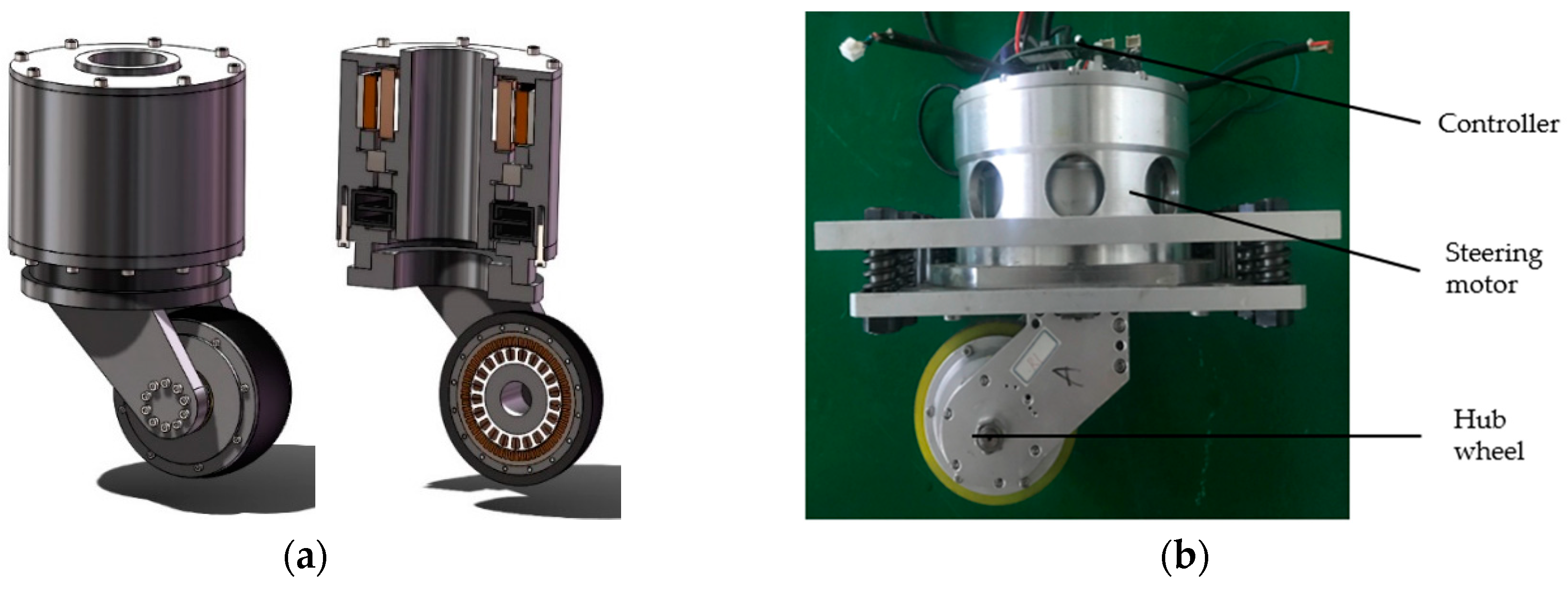
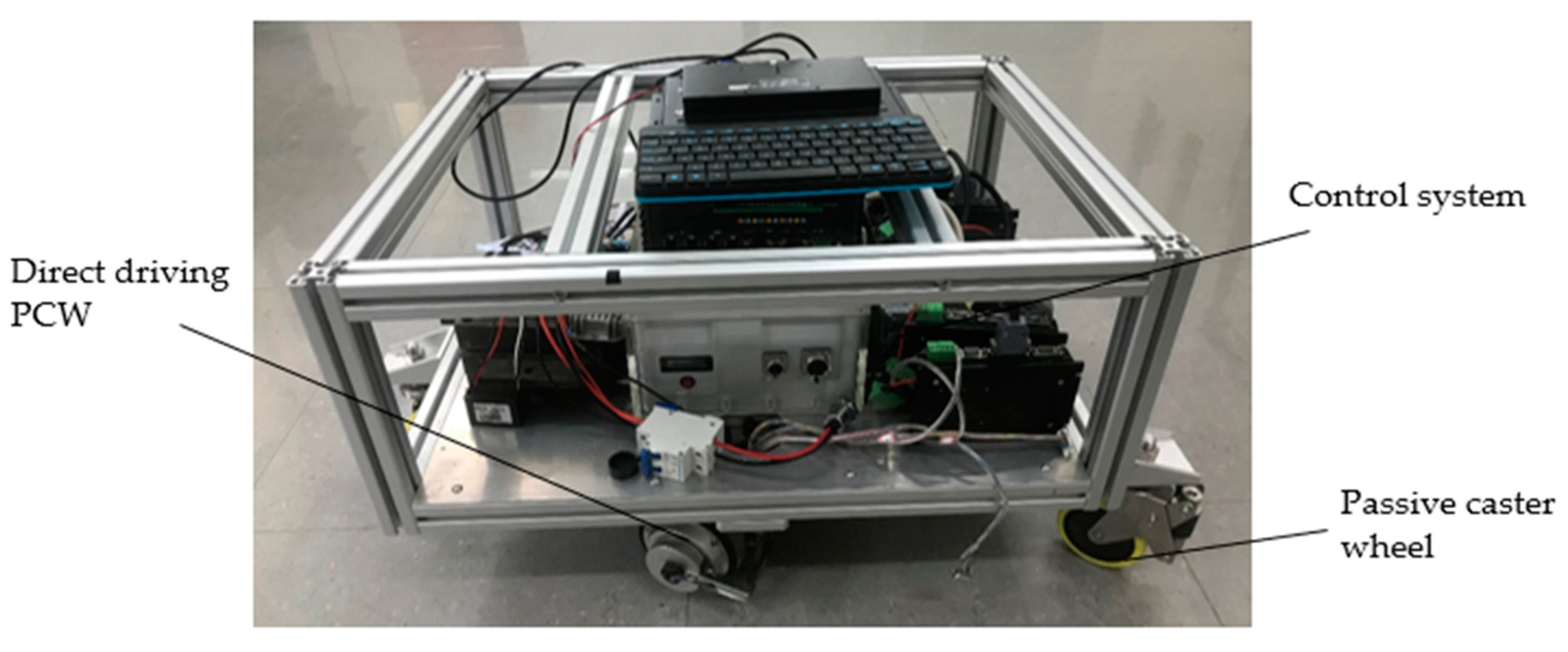
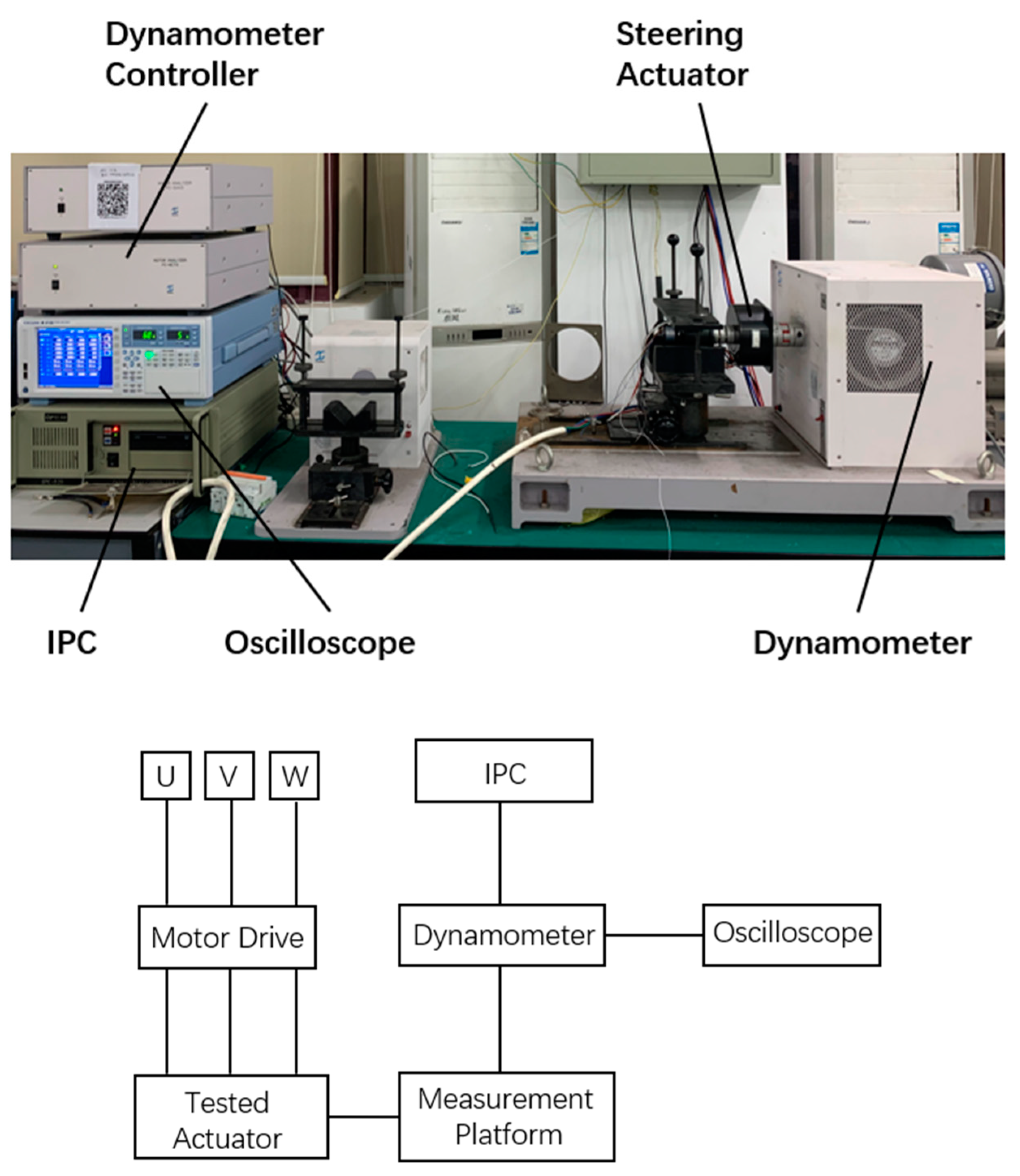
2. Design and Modelling of the OMR

The PCWs for the OMR are designed as a direct driving type. Two direct driving motors are integrated in a PCW, as shown in Figure 1. The upper motor is responsible for the steering motion, and the hub wheel motor is responsible for the rolling motion. All the PCWs are installed in the chassis of the OMR, the control system and other devices, such as the battery and sensors, are installed inside the mobile platform. By virtue of the direct driving PCWs, there is no transmission mechanism in the system, and the efficiency and stability of motion of the OMR are improved. Moreover, the PCW is integrated with less components, and the reliability of the direct driving PCW is also better than the conventional ones. The prototype of the OMR with two direct driving PCWs is shown in Figure 2.

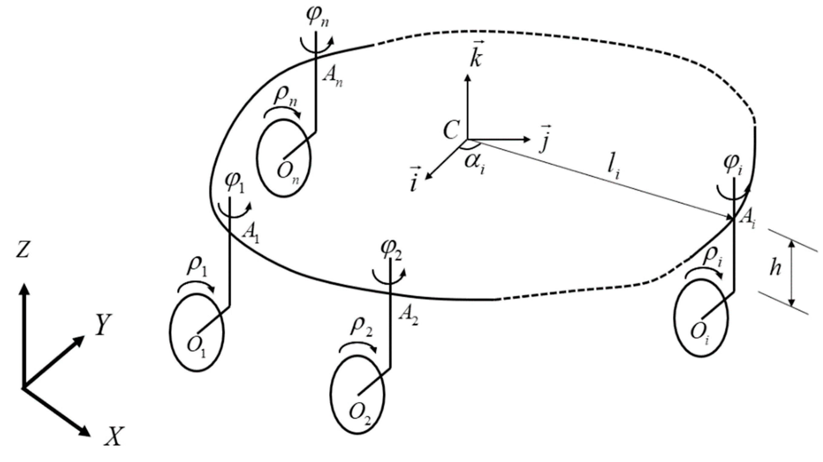
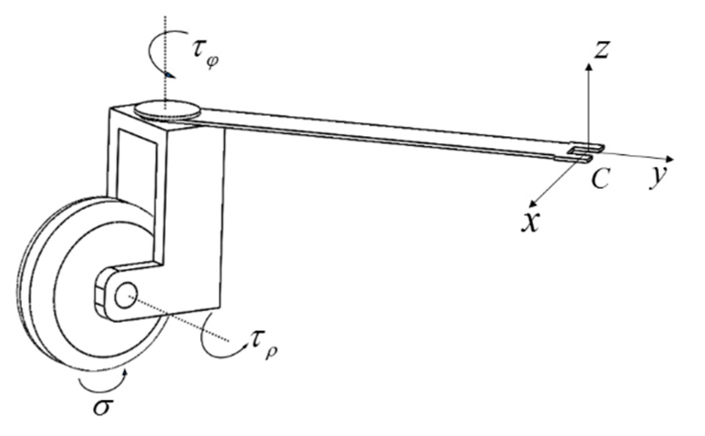
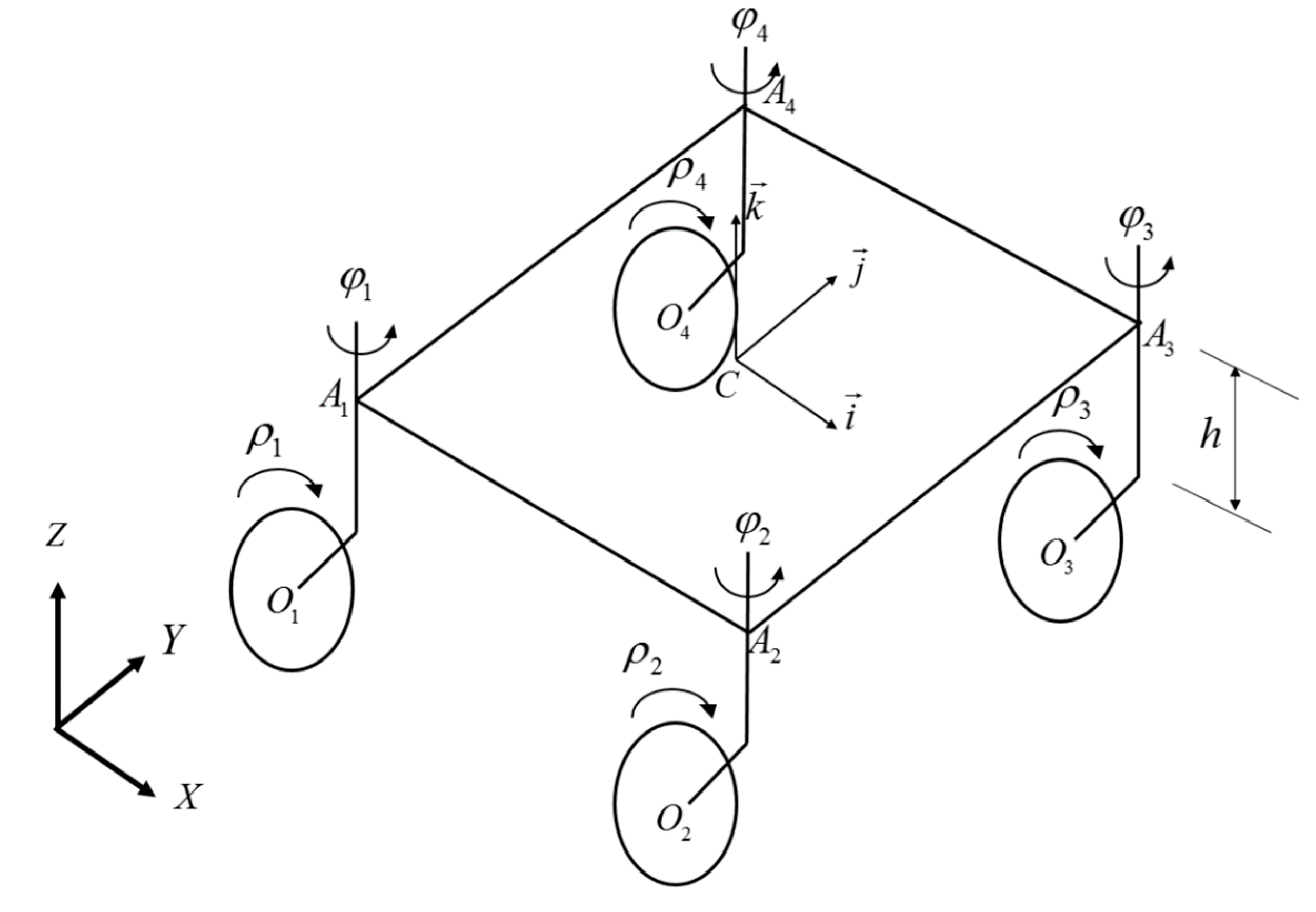
2.1. Kinematic Model of the OMR

The kinematic analysis of the OMR with PCWs will be presented in this section. Because the OMR moves on a horizontal surface, its motion can be described in a 2D frame. The OMR is designed in a modular pattern, which means we can choose the appropriate number of PCWs as well as their installing positions according to specific task requirements. A schematic diagram that illustrates the kinematic model of that modular designed OMR is presented in Figure 3. We assume that there are n-PCWs installed in the chassis of the OMR, and the points $A_i\left(i=1,2,\cdots ,n\right)$ represent the install positions for the PCWs, which are also called support points. The support points can also be regarded as the distal ends of the PCWs. A PCW is actuated by two active joints, which are responsible for the rolling motion and steering motion, respectively. It can produce a driving wrench $F_i^w={\left(f_{x_i},f_{y_i},m_{z_i}\right)}^T\left(i=1,2,\cdots ,n\right)$ to the support point in the platform. The resultant forces by all PCWs will drive the OMR to perform the desired trajectory.

The global reference frame XYZ is used to describe the configuration of the OMR, and $\overrightarrow{i},\overrightarrow{j},\overrightarrow{k}$ represent the three orthogonal axes of the local frame attached to the platform. As long as the number of PCWs is no less than two for singularity avoidance [20], the proposed kinematic analysis for the modular OMR is not restricted by the number of PCWs. Conventionally, the PCWs are arranged symmetrically for good dynamic performance and increasing the number of PCWs can improve the load capacity of the OMR. It should be noted that the kinematic model in this paper refers to the instantaneous kinematics, which maps the joint velocity $\dot{q}$ to the operational space velocity $\dot{x}$. As shown in Figure 3, ${\rho }_i\left(i=1,2,\cdots ,n\right)$ are defined as the rolling angles of the wheels and ${\phi }_i$ are defined as the steering angles; ${\sigma }_i$ are defined as the angular displacements of the ith wheels with respect to the X-axis. r denotes the wheels’ radius and b denotes the offset of the PCW, l is the vector for the center of the OMR to the support point, and α is the angle between l and $\overrightarrow{i}$. Then for the ith PCW, the linear speed at the center of the platform can be derived by

$$\begin{array}{ll}{v}_C& =v_{O_i}+\dot{\sigma }k\times O_i{A}_i+\omega k\times A_{i}C\\ & ={\dot{\rho }}_i(\sin {\phi }_{i}i+\cos {\phi }_{i}j)\times rk\\ & +\dot{\sigma }k\times (-b\cos {\phi }_{i}i+b\sin {\phi }_{i}j+hk)\\ & +\omega k\times (l\sin {\alpha }_{i}i+l\cos {\alpha }_{i}j)\end{array}.$$

(1)

Note that $\omega$, representing the angular velocity of the OMR, can be computed by

$$\omega =\dot{\sigma }+\dot{\phi }.$$

(2)

Combining (1) and (2), the kinematics of a PCW can be expressed in a single matrix form written as

$$\left[\begin{array}{c}{v}_x\\ v_y\\ \omega \end{array}\right]=\left[\begin{array}{ccc}-b\sin {\phi }_i-l\sin {\alpha }_i& r\cos {\phi }_i& -l\sin {\alpha }_i\\ b\cos {\phi }_i+l\cos {\alpha }_i& r\sin {\phi }_i& l\cos {\alpha }_i\\ 1& 0& 1\end{array}\right]\left[\begin{array}{c}{\dot{\sigma }}_i\\ {\dot{\rho }}_i\\ {\dot{\phi }}_i\end{array}\right].$$

(3)

Equation (3) presents the forward kinematic model of wheel $i$ and the kinematic models of the rest of the wheels can be derived in the same manner. The single castor wheel Jacobian matrix $J_i$ is always full rank as its determinant remains a nonzero constant. Thus, the inverse matrix of $J_i$ always exists.

In practice, it would be difficult to measure or control ${\sigma }_i$ as it represents a passive rotational motion. This variable needs to be eliminated from the inverse kinematics of a single PCW. The controllable joint velocity denoted by $q_i$, including steering and rolling variables only, can be expressed as

$${\dot{q}}_i=\left[\begin{array}{c}{\dot{\rho }}_i\\ {\dot{\phi }}_i\end{array}\right]=C_i\left[\begin{array}{c}{v}_x\\ v_y\\ \omega \end{array}\right],$$

(4)

where $C_i$ is called the wheel constraint matrix [16] because it describes the constraints at each contact point between the wheel and the ground. All wheels’ equations are combined to get the unified inverse kinematics, as follows:

$$C=\left[\begin{array}{c}{C}_1\\ C_2\\ ⋮\\ C_n\end{array}\right],\dot{q}=\left[\begin{array}{c}{\dot{q}}_1\\ {\dot{q}}_2\\ ⋮\\ {\dot{q}}_n\end{array}\right]=C\dot{x}.$$

(5)

2.2. Joint Space Dynamic Model of the OMR

In order to formulate the dynamic model of the entire system, the dynamic model of a single PCW should first be obtained. In Figure 4, the schematic model of the PCW is presented. A PCW consists of three main components: a wheel, a bracket, and a “virtual” link from the upper side of the bracket to the mass center of the OMR. We call the link “virtual” because it only exists conceptually. The PCWs are installed directly in the chassis of the robot. The virtual link just provides the position information of the support points from the mass center of the robot.

The equation of motion for a PCW can be obtained through the Lagrangian method. The OMR can only achieve planner motion, hence there only exists kinetic energy $K_i$. The rolling motion ${\dot{\rho }}_i$ is always orthogonal to the steering motion ${\dot{\phi }}_i$, thus they can be decoupled and calculated by

$$K_i=\frac{I_r{\dot{\rho }}_i^2}{2}+\frac{I_s{\dot{\phi }}_i^2}{2}+\frac{m_w{({\dot{\rho }}_{i}r)}^2}{2},$$

(6)

where $I_r$ is the inertial moment of the wheel about its rolling axis, $I_s$ is the inertial moment of the PCW about the steering axis, and $m_w$ is the mass of the PCW. The dynamic model of a PCW in the joint space can be derived as

$$\frac{d}{dt}\frac{\partial K_i}{\partial {\dot{q}}_i}-\frac{\partial K_i}{\partial q_i}=\left[\begin{array}{c}{\tau }_{{\rho }_i}\\ {\tau }_{{\phi }_i}\end{array}\right].$$

(7)

Because $K_i$ is only in regard to ${\dot{q}}_i$, $\partial K_i/\partial q_i=0$ holds. The dynamic model of a single PCW can be formulated as

$$M_i{\ddot{q}}_i={\tau }_i-{\tau }_{f_i}+P_i^T(-F_i^w),$$

(8)

where

$$M_i=\left[\begin{array}{cc}{I}_r+m{r}^2& 0\\ 0& I_s\end{array}\right],$$

$${\ddot{q}}_i=\left[\begin{array}{c}{\ddot{\rho }}_i\\ {\ddot{\phi }}_i\end{array}\right],$$

$$P_i^T=\left[\begin{array}{ccc}-r\cos {\phi }_i& b\sin {\phi }_i& 0\\ 0& 0& 1\end{array}\right].$$

In (8), ${\tau }_i$ represents the actuating torques and ${\tau }_{f_i}$ denotes the friction torques, which consist of Coulomb friction and viscous friction. $P_i$ is the matrix that maps the $i\mathrm{th}$ joint velocity to the support point velocity, and $-F_i$ is the external wrench applied by the platform.

The platform of the OMR can then be regarded as a manipulated object by the PCWs. The force resulted from the distal end of $i\mathrm{th}$ PCW is $F_i^w$. The dynamic model of the platform only can be expressed as

$${\Lambda }_p\ddot{x}+{\mu }_p(x,\dot{x})=F_o^w,$$

(9)

where ${\Lambda }_p=diag\left[\begin{array}{ccc}{m}_o& m_o& I_o\end{array}\right]$ is the inertial term of the platform, and ${\mu }_p(x,\dot{x})$ is the Coriolis and centrifugal term. $F_o^w$ is the resultant force applied by all the PCWs.

2.3. Operational Space Dynamic Model of the OMR

The operational space dynamic model of a PCW is expressed in the form as

$${\Lambda }_i\ddot{x}+{\mu }_i=F_i,$$

(10)

where ${\Lambda }_i=C_i^T{M}_i{C}_i$ is the operational space mass matrix, ${\mu }_i=C_i^T{M}_i{\dot{C}}_i$ is the operational space Coriolis and centripetal terms, and $F_i$ is the operational space wrench. The OMR is assumed to move in a plane surface, so the gravity component is neglected here.

After deriving the dynamic models of the PCWs, the augmented object model (AOM) [21] can be employed to obtain the dynamic model of the entire system. The AOM declares that the systematic dynamic model of the entire system in operational space can be obtained by adding all the operational space dynamics of the PCWs and the platform only at the operational space frame. Thus, the augmented mass matrix ${\Lambda }_{\oplus }$ and Coriolis and centripetal terms ${\mu }_{\oplus }$ of the OMR are given as

$${\Lambda }_{\oplus }={\displaystyle \sum _{i=1}^n{\Lambda }_i+{\Lambda }_p},$$

(11)

$${\mu }_{\oplus }={\displaystyle \sum _{i=1}^n{\mu }_i+{\mu }_p},$$

(12)

where ${\Lambda }_p$ and ${\mu }_p$ are the mass matrix and the Coriolis and centripetal terms of the platform only expressed in the operational space, respectively. $F$ is the resultant wrench applied to the OMR, expressed in the operational space frame. Finally, the operational dynamics of the OMR can be written as

$${\Lambda }_{\oplus }\ddot{x}+{\mu }_{\oplus }=F.$$

(13)

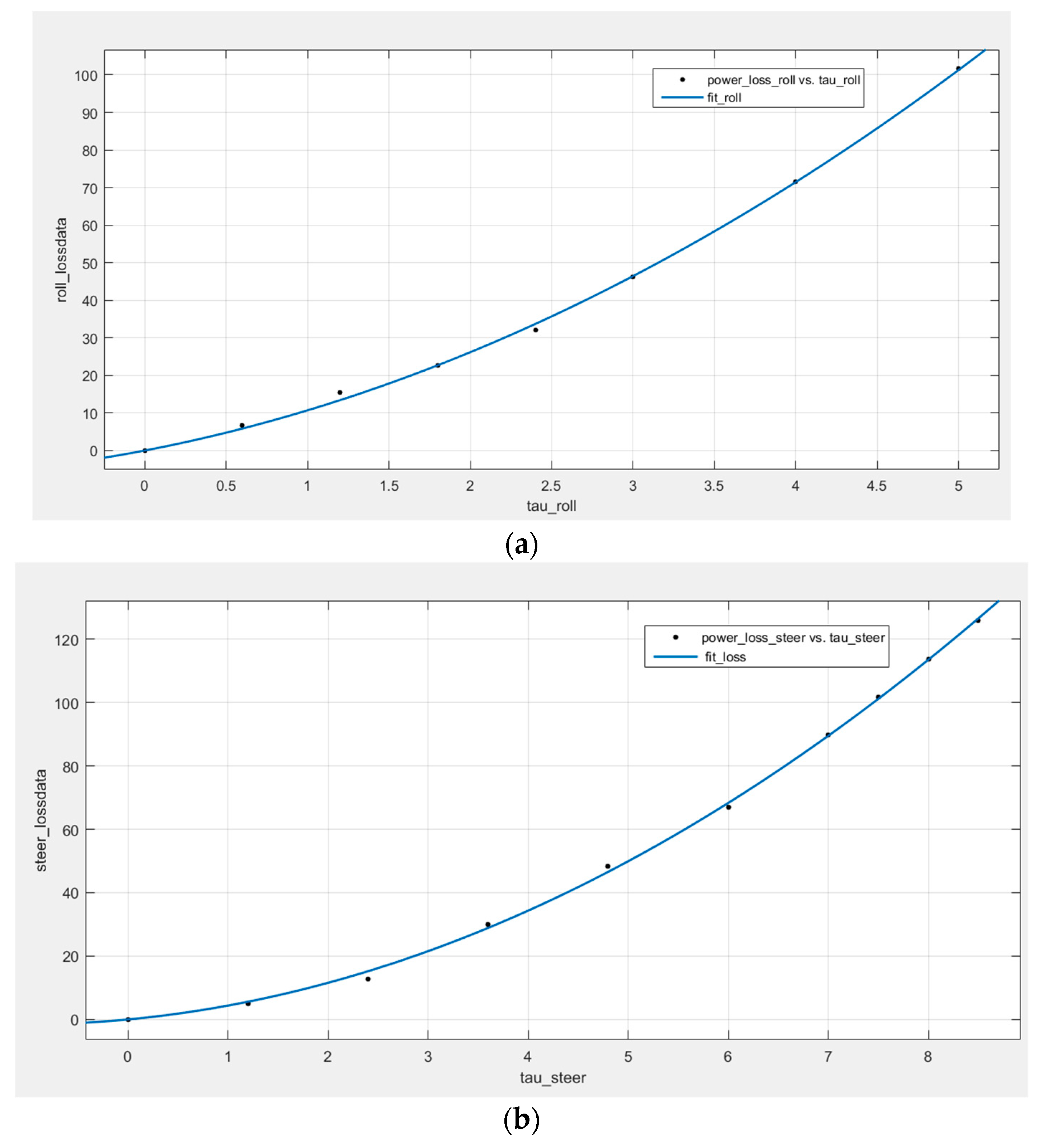
3. Energy Consumption Model of the OMR

The intact energy consumption model of the OMR consists of three parts: the sensors, the control system, and the motion system. The motion system consumes the overwhelming majority of energy in the OMR [10]. Hence, we mainly focus on the study of the influence of torque distributions to the energy consumption. The energy consumptions of the sensor system and the control system will not be discussed here. The formulation of energy consumption model is for predicting and evaluating the amount of energy consumed by the actuators in the OMR. The energy consumption can be calculated by integrating the power consumption about time. The power consumption model usually consist of output power consumption $P_{output}$ and the subordinate electrical power loss $P_{loss}$ [22,23].

$$P_{total}=P_{output}+P_{loss},$$

(14)

where the output power consumption is the power consumed to attain and sustain the desired motion of the OMR, and refers to the mechanical power. $P_{output}$ can be computed by

$$P_{output}={{\displaystyle \sum _{i=1}^n\left[{\tau }_i{\dot{q}}_i\right]}}^{\ast }.$$

(15)

The definition of ${[a]}^{\ast }$ is that, if a is larger than zero, the value of ${[a]}^{\ast }$ is a. If a is smaller than zero, the outcome value of the function is zero. It means that the negative output power cannot be regenerated and is dissipated as heat [24].

The electrical power loss often contains three parts: coil loss, conduction loss, and switching loss. The coil loss results from the heat dissipation as the current flows through the resistances of a circuit. It is formulated as follows:

$$P_{coil}={\displaystyle \sum _{i=1}^n{R}_i{I}_i^2},$$

(16)

where R_i is the resistance of the coil in the ith actuator. I_i is the current the of the ith actuator. The other two types of electrical power loss that happen in servo-amplifiers or servo-drives, including conduction loss and switching loss. Each loss happens when the current flows in an insulated-gate bipolar transistor of the servo-amplifier [25]. The conduction loss and switching loss are often formulated according to the voltage and current information. The literature of [25] provides a scheme for calculating the conduction and switching loss only dependent on the current information. The conduction loss and the switch loss can be expressed, respectively, by:

$$P_{conduction}={\displaystyle \sum _{i=1}^n{\mu }_i^a}{I}_i+{\mu }_i^b{I}_i^2,$$

(17)

$$P_{switching}={\displaystyle \sum _{i=1}^n{\eta }_i{I}_i},$$

(18)

where ${\mu }_i^a$ and ${\mu }_i^b$ are the coefficients for the conduction loss. The conduction loss is formulated in a quadratic polynomial manner with respect to the current. ${\eta }_i$ is the constant coefficient of switching with respect to the current. Hence, the electrical power loss can be computed by summing the coil loss, conduction loss, and switching loss.

$$P_{loss}=P_{coil}+P_{conduction}+P_{switching}.$$

(19)

All kinds of losses are formulated as the functions of current. By summing the coefficients according to the power of the current, the power loss can be expressed as

$$P_{loss}={\displaystyle \sum _{i=1}^n\left({\lambda }_i^a{I}_i+{\lambda }_i^b{I}_i^2\right)},$$

(20)

where ${\lambda }_i^a={\mu }_i^a+{\eta }_i$, and ${\lambda }_i^b={\mu }_i^b+R_i$. ${\lambda }_i^a$ and ${\lambda }_i^b$ are the coefficients of the power loss of the $i\mathrm{th}$ actuator in terms of the current.

Because we mainly investigate the relationship between the torque distributions and the energy consumption in this paper, it is desired to express the power consumption in the manner of joint torques. Fortunately, for the torque motors employed in the PCWs, their outputs are linearly proportional to the current in the circuit. Therefore, the current term $I_i$ and $I_i^2$ in (20) can be replaced by the torque term ${\tau }_i$ and ${\tau }_i^2$ with their corresponding linear coefficients. Equation (20) can be reformulated as

$$P_{loss}={\displaystyle \sum _{i=1}^n\left({\kappa }_i^a\left|{\tau }_i\right|+{\kappa }_i^b{\tau }_i^2\right)},$$

(21)

where ${\kappa }_i^a$ and ${\kappa }_i^b$ are the coefficients for the electrical power loss of the absolute value of torque and the square of torque in the $i\mathrm{th}$ actuator, respectively. The new electrical power loss model (21) in terms of the torque represents a combination of the electrical power loss model in terms of the current and the linear proportional relationship between the current and the torque in the actuator.

After obtaining the output power consumption model of the OMR, the coefficients of the model have to be specified via experimental measurement. For accuracy, the angular velocities of the actuators are set to be constant, and photoelectric encoders on the motors can be used to measure the velocities of motors and provide feedback to the control system in real time [10]. A strain-gauge sensor [24] is employed to measure the torque of each actuator. The coefficients in (21) are acquired through the power measurement while different static loads are applied to each actuator, and the experiment is executed as shown in Figure 5. The power measurement is implemented by a dynamometer (SUGAWARA PC-MCT6). The tested actuator is connected to the dynamometer by a shaft coupling. The industrial personal computer (IPC) is responsible for controlling and sending commands to the dynamometer. The actuator is commanded to rotate in constant angular velocity with several static loads induced by the dynamometer, and the real-time voltage and current of the actuator are shown in the oscilloscope (YOKOGAWA WT1800). The output power of the actuator can be calculated by multiplying its angular velocity and the output torque applied by the dynamometer. Figure 6a,b shows the experimental result of electrical power loss of the rolling actuator and the steering actuator with respect to different loads, respectively. The markers are measurement points of the experiment. The coefficients of the power consumption models are obtained through mathematical curve fitting by MATLAB by (21), and the results are shown in

Table 1. Experimental results for the coefficients of the power loss model.

Class of Actuators	${\mathit{\kappa }}_{\mathit{i}}^{\mathit{a}}$	${\mathit{\kappa }}_{\mathit{i}}^{\mathit{b}}$
Steering actuator	2.98	1.40
Rolling actuator	3.39	2.31

.

From the above, the total power consumption of the motion system can be written as

$$P_{total}={{\displaystyle \sum _{i=1}^n\left[{\tau }_i{\dot{q}}_i\right]}}^{\ast }+{\displaystyle \sum _{i=1}^n\left({\kappa }_i^a\left|{\tau }_i\right|+{\kappa }_i^b{\tau }_i^2\right)}.$$

(22)

The energy consumption model for the OMR can be calculated by

$$E\left(\tau \right)={\displaystyle \underset{t_0}{\overset{t_f}{\int }}\left({{\displaystyle \sum _{i=1}^n\left[{\tau }_i{\dot{q}}_i\right]}}^{\ast }+{\displaystyle \sum _{i=1}^n\left({\kappa }_i^a\left|{\tau }_i\right|+{\kappa }_i^b{\tau }_i^2\right)}\right)}.$$

(23)

Each PCW has two motors for rolling and steering motions, respectively, so the number $n$ is $2m$ for the OMR with $m$ PCWs.

4. Torque Distribution Schemes for the OMR

The torque distribution schemes of robots can be derived from the forward kinematic model by

$$\tau =J^{T}F,$$

(24)

where $\tau$ is the actuating torques applied by the joints and $J$ is the Jacobian matrix of the robot. In the analysis of the torque distribution for the OMR, because the PCWs are direct driven, the impact of the transmission system in the PCWs and the dynamics of the motors are neglected. We assume that the torques produced by the actuators are the same torques applied to the joints. Owing to the parallel structure and redundant actuation of the OMR, the Jacobian matrix cannot be derived directly through kinematics analysis. Instead, it is obtained by computing the generalized inverse of the constrained matrix C of the OMR [15]. This means that if the task space velocity of the OMR is given, the joint velocity can be directly calculated by the constraint matrix. However, the task space velocity cannot be obtained from arbitrary joint velocity because of the kinematic constraints. The constraint matrix maps the operational space velocity $\dot{x}$ to the joint space velocity $\dot{q}$ by

$$\dot{x}=C\dot{q}.$$

(25)

The Jacobian matrix of the OMR can be obtained by computing the generalized inverse matrix of the constraint matrix:

$$J=C^{+}.$$

(26)

Because the OMR is redundantly actuated, the constraint matrix $C$ is not square. Hence, there exists a non-unique Jacobian matrix for the OMR, and the different choices of the generalized inverse will lead to different torque distribution schemes.

4.1. Torque Distribution Schemes Resulting from the Generalized Inverse of the Jacobian

Two reasonable determinations of torque distribution schemes proposed by the published research [17] are first presented. The kinematics of the OMR with PCWs can be expressed in an equivalent way as

$$A\dot{x}=B\dot{q},$$

(27)

where $B$ is a diagonal matrix and $A$ is a non-square matrix. The first torque distribution scheme is expressed as

$$\tau ={\left(B^{-1}A\right)}_{LPI}^{T}F,$$

(28)

where ${\left(B^{-1}A\right)}_{LPI}$ means computing the left Moore–Penrose pseudo-inverse of $B^{-1}A$. Using this model, the joint torque differences are minimized in a least-squares manner. The second torque distribution scheme is expressed as

$$\tau =B^T{A}_{LPI}^{T}F,$$

(29)

where $A_{LPI}$ means computing the left Moore–Penrose pseudo-inverse of $A$. Using this model, the joint torque as well as the interaction forces between different contact points are minimized, in a least-squares manner.

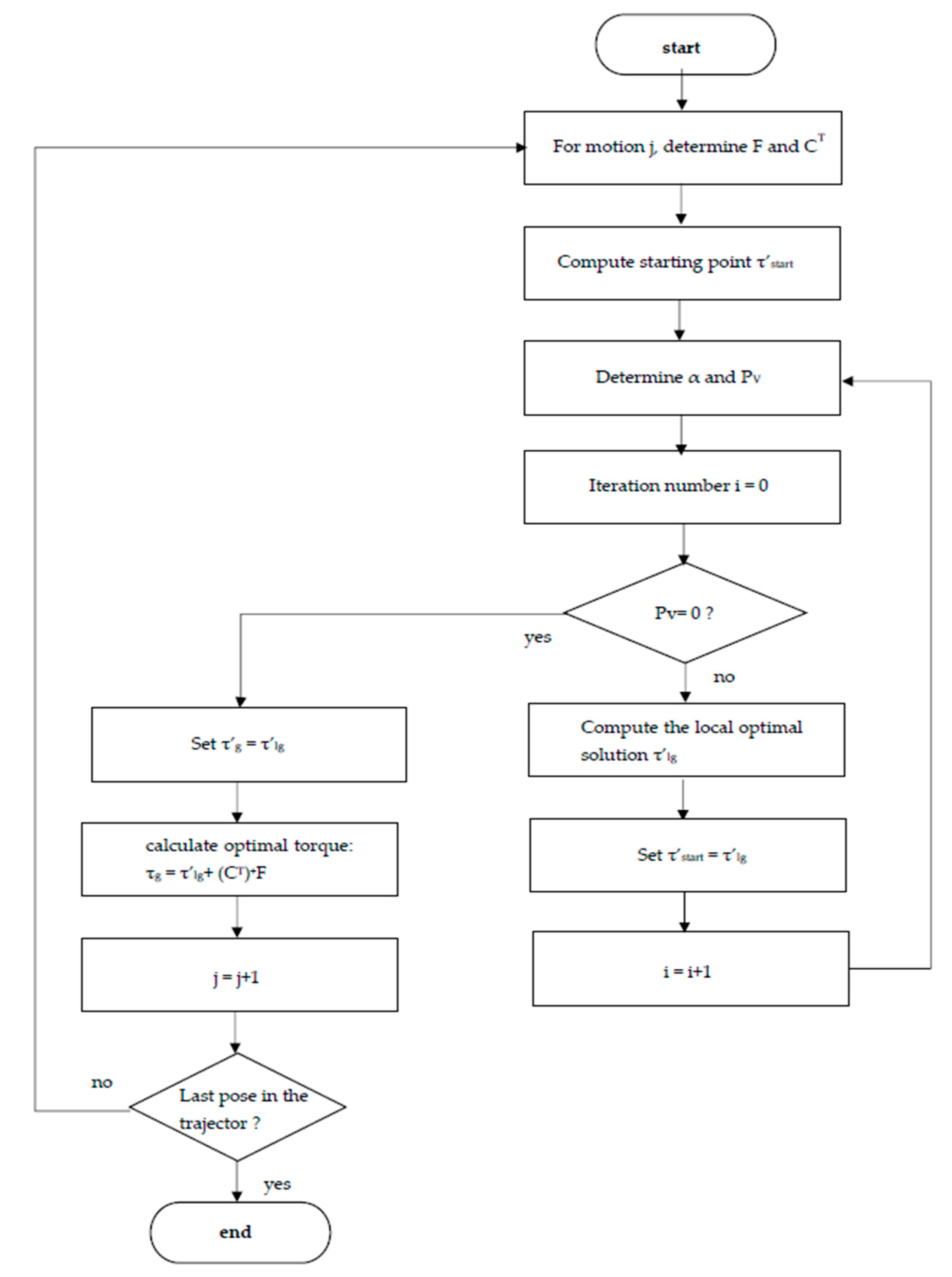
4.2. Gradient Projection-Based Torque Optimization

The gradient projection method is an efficient and widely-employed optimization method in the control of redundant robots [26,27]. It fully utilizes the null space of the Jacobian matrix to optimize varieties of performance criteria, such as manipulability, obstacle avoidance, and joint limit avoidance. It is approached by projecting the steepest descent direction of the performance criterion onto the null space and finding the best solution along the projected vector. The flowchart of the proposed torque distribution optimization algorithm is shown in Figure 7. For the torque distribution of the redundant actuated OMR, as mentioned before, the joint space torque is not directly projected from the operational space force by the transpose of the Jacobian matrix, but instead of the constraint matrix $C$, written by

$$C^T\tau =F.$$

(30)

As the 3-DOF OMR is actuated by $m\left(m\ge 4\right)$ actuators, the joint torques can be expressed as

$$\tau ={(C^T)}^{+}F+\left[I-{(C^T)}^{+}{C}^T\right]v,$$

(31)

where $v\in R^m$ is an arbitrary vector. On the basis of GPM, it can be replaced by the gradient of a performance criterion $H\left(\tau \right)$, which yields

$$\tau ={(C^T)}^{+}F+k\left[I-{(C^T)}^{+}{C}^T\right]\nabla H\left(\tau \right),$$

(32)

where k is the searching step size and $\nabla H\left(\tau \right)$ is the gradient of $H\left(\tau \right)$. Note that scalar $k$ is positive if $H\left(\tau \right)$ needs to be maximized and is negative if $H\left(\tau \right)$ needs to be minimized. The detailed construction of $H\left(\tau \right)$ for the optimization will be presented later.

In order to implement GPM to the torque distribution of the OMR, the torque limits have to be determined first. The limit of the torque ${\tau }_{\max }$ and ${\tau }_{\min }$ is determined by two factors: the maximum and minimum produced torques of the actuator ${\tau }_{motor\max }$ and ${\tau }_{motor\min }$; and the maximum ground traction ${\tau }_{traction}$, which is expressed below:

$$\begin{array}{l}{\tau }_{traction}=N\cdot \left({\mu }_c+{\mu }_{v}v\right)\cdot sign\left(v_c\right)\\ {\tau }_{\max }=\min \left({\tau }_{motor\max },{\tau }_{traction}\right)\\ {\tau }_{\min }=\max \left({\tau }_{motor\min },-{\tau }_{traction}\right)\end{array},$$

(33)

where $N$ is the ground contact force of the wheel, ${\mu }_c$ is the Coulomb friction coefficient, ${\mu }_v$ is the viscous friction coefficient, and $v_c$ is the velocity of the wheel at the wheel-ground contact point. In practice, the maximum ground traction is smaller than the maximum produced torque, which means that, during the motions of the OMR, the actuating torques may exceed the ground traction and, consequently, slippage happens to the wheels. Employing the limit of the actuating torques and rewriting (22), it yields the following:

$$\begin{array}{c}\tau -{(C^T)}^{+}F=k\left[I-{(C^T)}^{+}{C}^T\right]\nabla H\left(\tau \right)\\ {\tau }_{\min }-{(C^T)}^{+}F\le k\left[I-{(C^T)}^{+}{C}^T\right]\nabla H\left(\tau \right)\le {\tau }_{\max }-{(C^T)}^{+}F\end{array}.$$

(34)

Let ${\tau }^{\prime }=\tau -{(C^T)}^{+}F$, where ${\tau }^{\prime }$ is a point in the null space of $C^T$, then the optimization problem can be expressed as

$$\begin{array}{l}Objective\mathrm{function}:H\left({\tau }^{\prime }\right)\\ Subjected{\mathrm{to}:\mathrm{C}}^{+}{\tau }^{\prime }=0\\ {\tau }_{\min }-{(C^T)}^{+}F\le {\tau }^{\prime }\le {\tau }_{\max }-{(C^T)}^{+}F\end{array}.$$

(35)

Resolving the optimization problem of (35) will produce an optimal solution ${{\tau }^{\prime }}_g$ in the null space of $C^T$. After that, the optimal solution of ${\tau }_g$ can be obtained by ${\tau }_g={{\tau }^{\prime }}_g+{\left(C^T\right)}^{+}F$.

After defining the optimization problem of the actuating torques of the OMR, the performance criterion $H\left({\tau }^{\prime }\right)$ need to be formulated. The boundary conditions in (35) declare that ${\tau }^{\prime }$ must be within the feasible zone, which is away from the actuating torque limit. It can be expressed as

$$\begin{array}{c}{{\tau }^{\prime }}_{\min }\le {\tau }^{\prime }\le {{\tau }^{\prime }}_{\max }\\ \left({{\tau }^{\prime }}_{\min }={\tau }_{\min }-{(C^T)}^{+}F,{{\tau }^{\prime }}_{\max }={\tau }_{\max }-{(C^T)}^{+}F\right)\end{array}.$$

(36)

The performance criterion used to generate the feasible zone can be given as

$$H_{feasible\mathrm{zone}}{\left({\tau }^{\prime }\right)}_i=\frac{1}{\left[{\left({{\tau }^{\prime }}_{\max }\right)}_i-{\left({\tau }^{\prime }\right)}_i\right]\left[{\left({\tau }^{\prime }\right)}_i-{\left({{\tau }^{\prime }}_{\min }\right)}_i\right]},$$

(37)

where $i$ refers to the $i\mathrm{th}$ component of the corresponding torque vector. For such a performance criterion, the value of the function goes to infinity, while the actuating torque approaches either a maximal or minimal limit, and goes to minimal while the actuating torque reaches the midpoint of the feasible torque interval. This indicates that, while searching for the minimal point, the performance criterion will retain the actuating torque within the feasible torque zone and away from either the maximum or minimal limit. Hence, using this performance criterion, the maximal (or absolute value of minimal) required actuating torque of the OMR for a specific trajectory will be reduced.

In addition, it is our main purpose to take the energy consumption into account for the torque distribution of the OMR. Therefore, another term that resulted from (22) is introduced into the performance criterion, which is given as

$$\begin{array}{l}H\left({\tau }^{\prime }\right)={\displaystyle \sum _{i=1}^{m}H{\left({\tau }^{\prime }\right)}_i}\\ H{\left({\tau }^{\prime }\right)}_i=\frac{1}{\left[{\left({{\tau }^{\prime }}_{\max }\right)}_i-{\left({\tau }^{\prime }\right)}_i\right]\left[{\left({\tau }^{\prime }\right)}_i-{\left({{\tau }^{\prime }}_{\min }\right)}_i\right]}\ast \left[{\left[{{\tau }^{\prime }}_i{\dot{q}}_i\right]}^{\ast }+\left({\kappa }_i^a\left|{{\tau }^{\prime }}_i\right|+{\kappa }_i^b{{\tau }^{\prime }}_i^2\right)\right]\end{array}.$$

(38)

The modified performance criterion is used to optimize for a preference of better energy efficiency. It should be noted that the performance criterion function must be continuous while applying GPM, but the function in (38) is discontinuous at the point ${{\tau }^{\prime }}_i=0$. This issue can be solved by using a curve fitting polynomial function to replace the original function at a small interval $[-0.1,0.1]$ around ${{\tau }^{\prime }}_i=0$, with an acceptable sacrifice of accuracy.

Now, with the objective function given in (38), the optimization problem expressed in (35) becomes a convex optimization problem because both the objective function and the inequality constraints are convex. In this situation, using the GPM can always find the global optimal solution. The GPM is executed by the following equation:

$$\begin{array}{ll}{{\tau }^{\prime }}_{\lg }& ={{\tau }^{\prime }}_{start}-k{\left(\left[I-{(C^T)}^{+}{C}^T\right]\nabla H\left({{\tau }^{\prime }}_{start}\right)\right)}_{unit}\\ & ={{\tau }^{\prime }}_{start}-k{\left(P_v\right)}_{unit}\end{array},$$

(39)

where ${{\tau }^{\prime }}_{\lg }$ is the local optimal solution along the unit projective vector ${\left(P_v\right)}_{unit}$, ${{\tau }^{\prime }}_{start}$ is the starting point in the null space of $C^T$, and $k$ is the step size along ${\left(P_v\right)}_{unit}$. On the basis of the definition of gradient, ${\left(P_v\right)}_{unit}$ is obtained by projecting the steepest descent direction of the objective function onto the null space of $C^T$. In order to get the global optimal solution, set ${{\tau }^{\prime }}_{start}={{\tau }^{\prime }}_{\lg }$ and repeat (39) again and again. The global optimal solution ${{\tau }^{\prime }}_g$ will be obtained when the iteration stops at ${\left(P_v\right)}_{unit}=0$, indicating that the performance criterion has already come to its “lowest position”.

The last problem that needs to be coped with is the determination of the starting point ${{\tau }^{\prime }}_{start}$. The GPM will have a low computational cost and converge more rapidly if ${{\tau }^{\prime }}_{start}$ is closer to the global optimal solution. A simple, but effective method is to project the torque distribution in (29) onto the null space of $C^T$, and to set the result as the starting point for each motion in the entire trajectory, as the result in (29) has already been optimized in a least-squares manner. However, a more reasonable starting point in the current motion $j$ of the planned trajectory can be obtained by projecting the optimal solution of last motion $j-1$ onto the null space of the current motion $j$, expressed as

$${{\tau }^{\prime }}_{start\_j}=\left(I-{\left(C_j^T\right)}^{+}{C}_j^T\right){{\tau }^{\prime }}_{g\_j-1}.$$

(40)

As $F$ and $C^T$ are continuous, ${{\tau }^{\prime }}_{start\_j}$ will be very close to the new optimal solution ${{\tau }^{\prime }}_{g\_j}$ if ${{\tau }^{\prime }}_{g\_j}$ is the optimal solution in the last motion $j-1$.

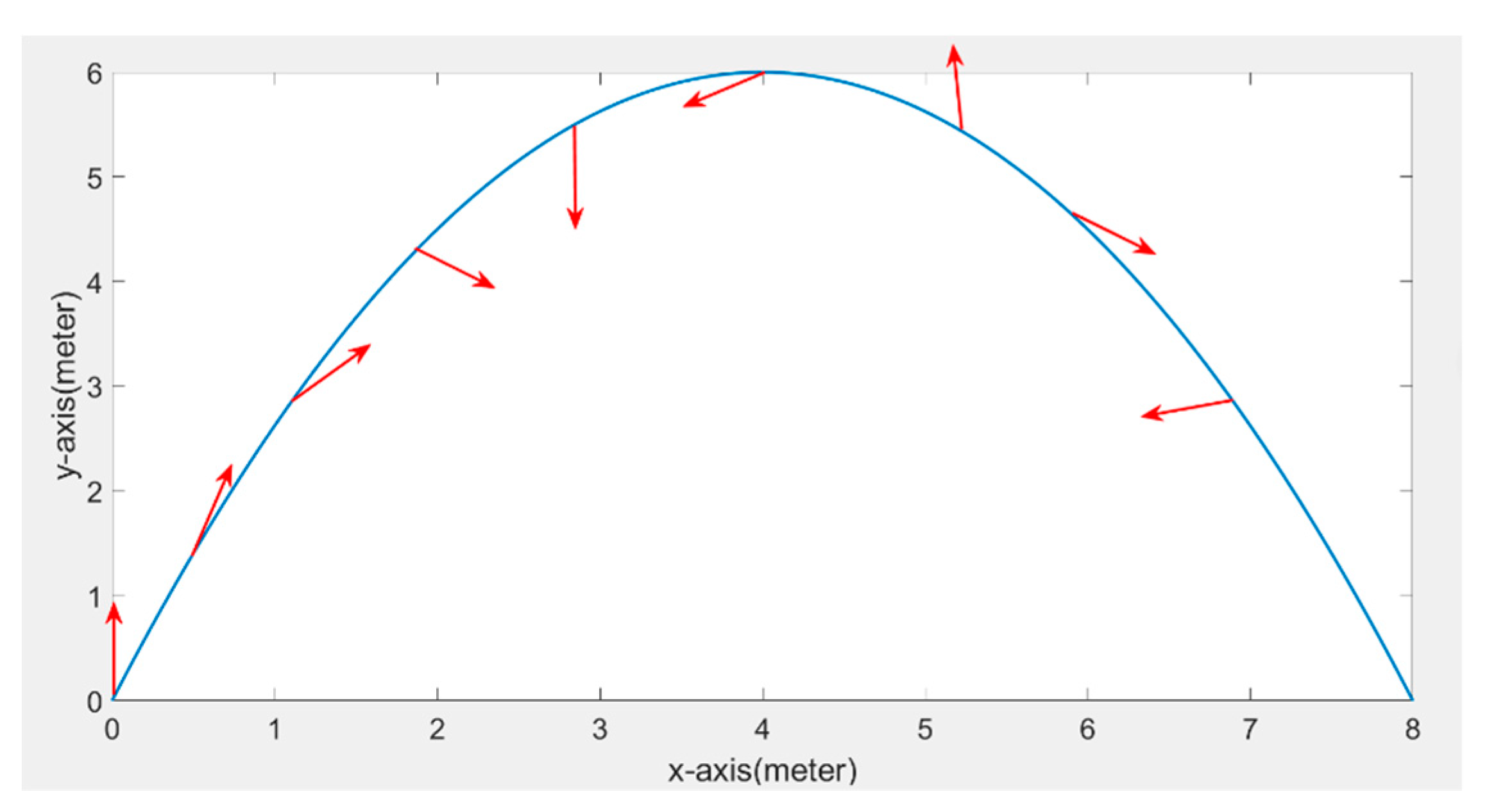
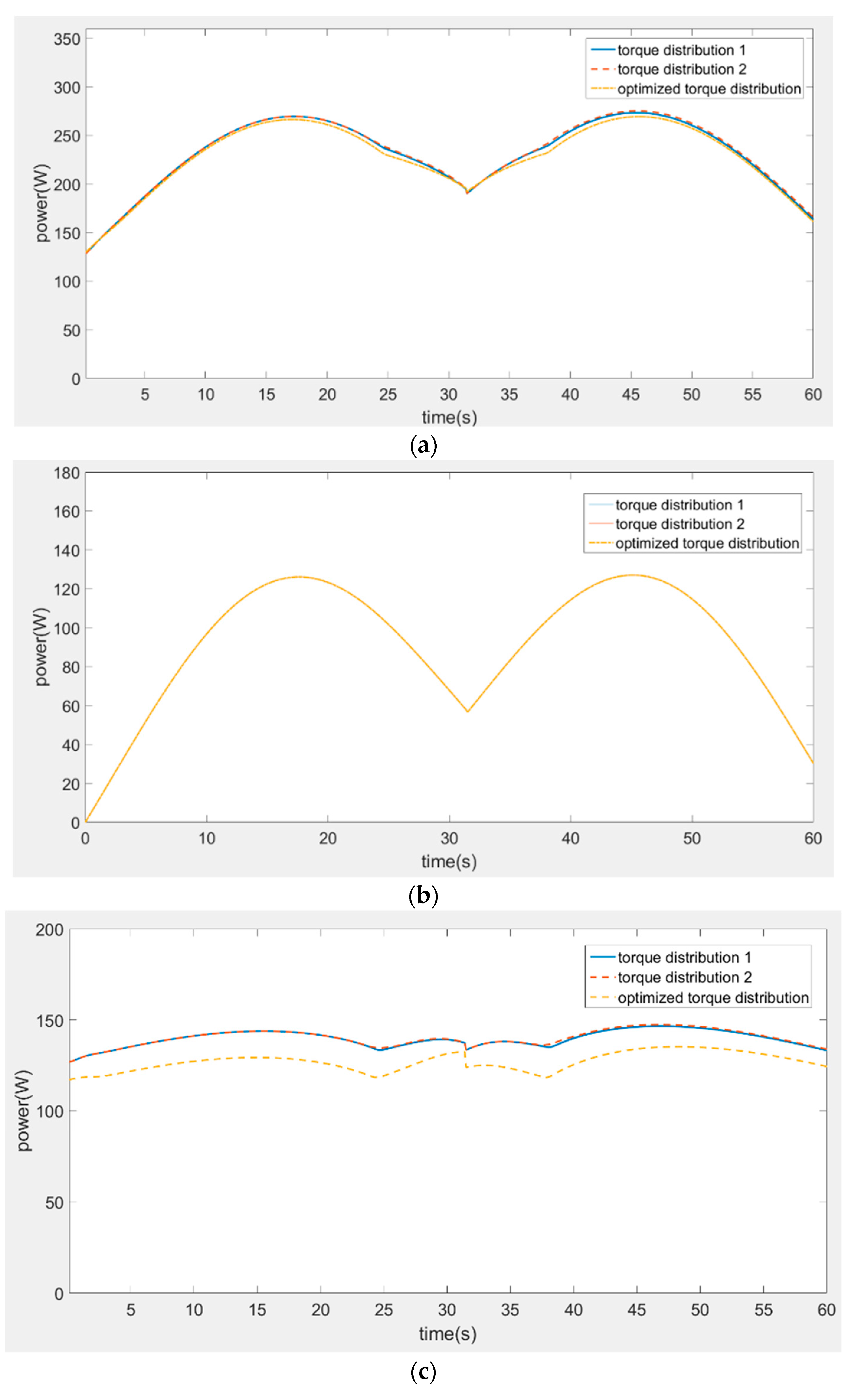
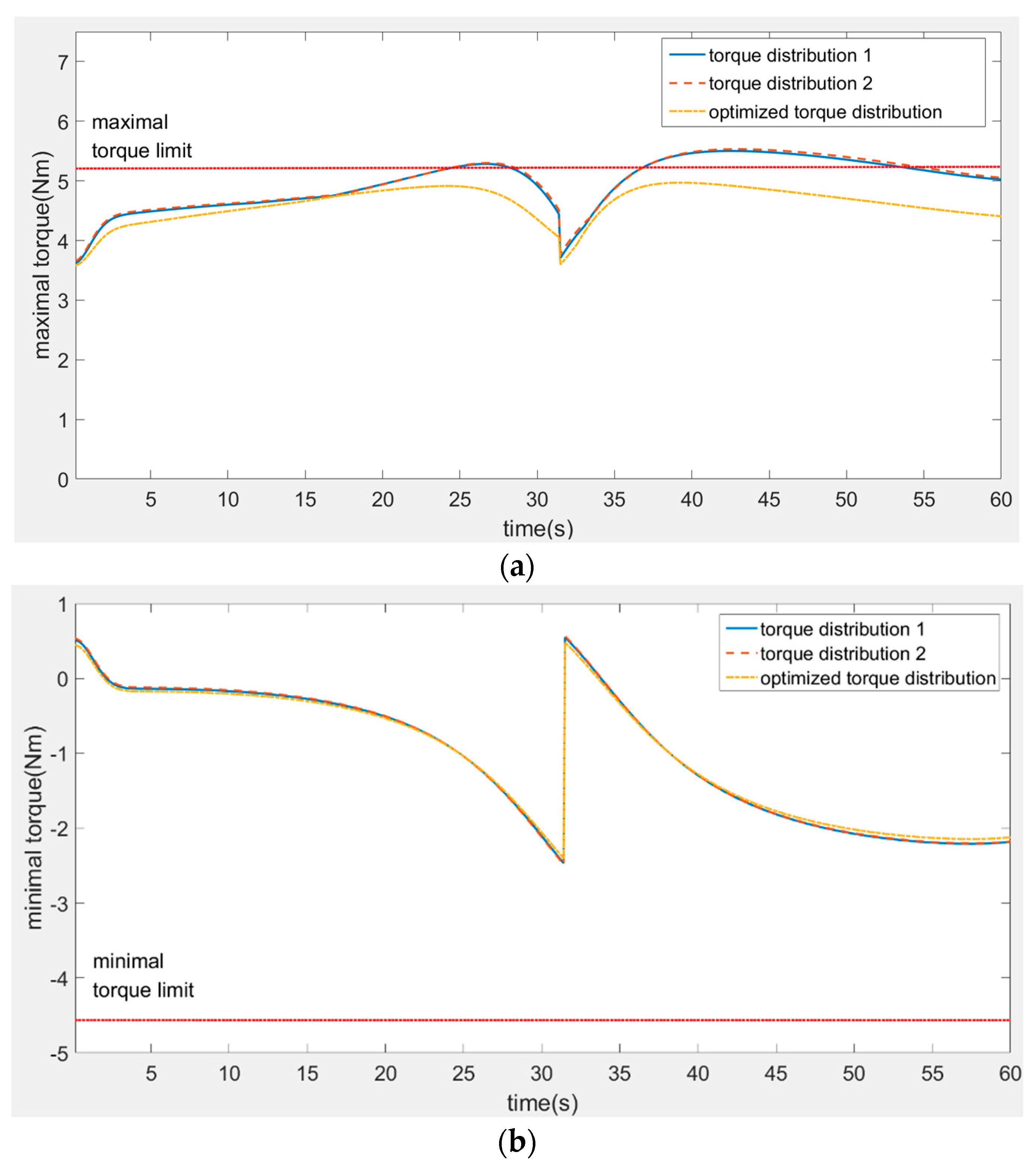
5. Simulation Examples and Results Analysis

The simulation is presented in this section for validating the effectiveness of the proposed optimization method by MATLAB (r-2015b version, MathWorksS, Natick, US). The OMR used for simulation is shown in Figure 8. All PCWs in the OMR are identical. The platform of the OMR is designed in squared shape, and each PCW locates at one of the four corners of the platform. The parameters of the OMR are given as follows: the mass of the platform without any PCWs is 52 kg, the side length L of the platform is 0.5 m, the radius of each wheel is 0.05 m, the offset of the castor wheel is 0.046 m, and the mass of each PCW is 5 kg. The coefficients of the electrical power loss are referred from the experimental results in Figure 6. The lower and upper bounds of the actuating torque are $\pm 6\mathrm{N}\cdot \mathrm{m}$ for the rolling motors and $\pm 8\mathrm{N}\cdot \mathrm{m}$ for the steering motors.

In order to further illustrate the results of the torque distribution optimization for the OMR with PCWs, a curvilinear trajectory is proposed next. The path is shown in Figure 9; the OMR moves from the original point to the endpoint, then turns around at the endpoint and moves back to the original point. The OMR is commanded to track the path with self-rotation for taking full advantage of holonomicity, and the red arrows in Figure 9 represent the head directions (vector $\overrightarrow{i}$ in Figure 8) of the OMR. The function of the trajectory is expressed as follows:

$$\{\begin{array}{l}\mathrm{x}=4-4\cos (\mathrm{t}/20);\left(\mathrm{meter}\right)\\ \mathrm{y}=3-3\cos (\mathrm{t}/10);\left(\mathrm{meter}\right)\\ \theta =3-3\cos (\mathrm{t}/15);\left(\mathrm{rad}\right)\end{array}.$$

(41)

Compared with the series manipulators, the mobile robots usually have much larger tracking errors, and one of the primary reasons for the tracking errors is the slippage between the wheels and the ground. The slippage is often difficult to predict because of the uncertainty of the ground conditions. However, because the phenomenon often occurs when the actuating torques of the wheels exceed the traction limit of the ground, reducing the maximal required actuating torques of the wheels during the performance of a specific trajectory can decrease the tendency of slippage. According to the normal indoor ground condition and the limits of the actuators, the maximal torque limits are calculated by (33) and set to be $\pm 5.3\mathrm{N}\cdot \mathrm{m}$ and $\pm 4.6\mathrm{N}\cdot \mathrm{m}$ for the rolling and steering actuators, respectively. Figure 10 shows the maximal required actuating torque among all PCWs during the motion, with both forward and backward rotation. The maximal positive actuating torque is significantly reduced by the optimization, by approximately 11% at the highest point compared with the former torque distribution Schemes 1 and 2 expressed in (28) and (29), respectively. The maximal negative actuating torque is also reduced by 6% at the highest point. Moreover, the red dotted lines represent the maximal positive and negative torque limits of the motors in the PCW. The maximal torque resulted from the former two torque distribution schemes exceed the torque limit. As it is difficult to simultaneously consider the torque limits when using the pseudoinverse method. In contrast, the optimized torque is totally below the limit. For such a trajectory, the actuators are commanded to produce less torques for the backward rotation, so that all three torques’ distributions have kept the maximal negative torques within the torque limits. For other joints with less actuating torques, the differences between the optimization outcomes and the results from pseudoinverse are not as significant as the differences shown in Figure 10. However, the torques of the other joints are still decreased to a smaller extent, and the data are not listed for concision. Figure 11 shows the power consumption of the OMR following the curvilinear trajectory adopting the three kinds of torque distribution schemes. As shown in Figure 11b,c, the power consumption is reduced by using the optimized torque distribution compared with the other two schemes, basically owing to the saving in electrical power loss part. The output power consumptions for the three torque distribution schemes are the same; because the OMR is commanded to follow the same trajectory by using the three different torque distribution schemes, the output power consumption that attains and sustains the motion of the OMR will be the same for the three cases. Besides being transferred into kinetic energy, the actuating torques are partly consumed to produce internal forces. The internal forces will be counteractive to each other and do not contribute to the motion of the OMR; the portion of the actuating torques corresponding to the internal forces still consumes energy in the actuators and is transformed to different kinds of losses expressed in (27). The total energy consumption as well as energy loss are presented in

Table 2. Simulation results of total energy consumption for the curvilinear trajectory.

Torque Distribution Scheme	Energy Loss (Joule)	Energy Consumption (Joule)
Optimized torque distribution	7.24 × 103	1.26 × 104
Torque distribution 1	8.37 × 103	1.38 × 104
Torque distribution 2	8.39 × 103	1.39 × 104

. By using the proposed optimization method, the total energy consumption can be reduced by 9.3% for the given trajectory.

Furthermore, the torque distribution optimization has to be computationally efficient if it is applied in real-time dynamic control. Because the optimization algorithm is iteration-based, the computational time is determined by the number of iterations per step. The step size of the continuous motion is discretized in every 0.1 second, and the average numbers of iterations per motion step are shown in

Table 3. Number of iterations per step.

Starting Point	[1,1,1,1,1,1,1,1]T (An Arbitrary Choice)	Pseudo-Inverse Solution	Proposed Method
Average number of iterations per step	79.24	19.57	4.86

. In order to reveal the superiority of the proposed method for determining the starting point expressed in (40), the results of the number of iterations from two other choices of starting point are also presented as a contrast. The first choice is an arbitrary simple point, and the second choice is the pseudo-inverse solution resulting from (29). The computational efficiency of the proposed method for determining the starting point is apparently approved.

6. Conclusions and Future Work

This paper presents the optimization of the torque distribution for the redundantly actuated OMR with PCWs based on GPM. The kinematic and dynamic models of the OMR are firstly formulated. In this paper, although the model used in simulation is an OMR with four PCWs, the modelling approach is in a modular way, which is suitable for the OMR with an arbitrary number of PCWs, as well as their mounting positions in the chassis. The detailed energy consumption model of the OMR including output energy consumption and electrical energy loss is then formulated, the the coefficients of the model are obtained by experimental test. Besides the energy consumption, the maximal required actuating torque to perform a specific trajectory is also non-negligible, as slippage often occurs when the actuating torques of the wheels exceed the ground traction limits. A performance criterion combined with torque limits and energy consumption is proposed in the GPM. Compared with two torque distribution schemes, which result from the Moore–Penrose pseudo-inverse method, the optimized torque distribution can significantly decrease the maximal required actuating torque as well as the total energy consumption, by 11% and 9.3%, respectively. Finally, the computational efficiency of the proposed optimization algorithm is validated. In further research, we intend to extend the torque distribution optimization method to an omnidirectional mobile manipulator, which means a serial manipulator is mounted on the OMR. While performing a task, the torque limit for each actuator of the PCW may change in real-time because the ground contact force of each PCW is related to the current configuration and motion of the manipulator. Moreover, the trajectory planning will become more complicated for that case, the motion of the OMR has to be decoupled from the motion of the entire system, and a multi-objective optimization method is expected to cope with the issues.

References

1. Yang, G.; Li, Y.; Lim, T.M.; Lim, C.W. Decoupled powered caster wheel for omnidirectional mobile platforms. In Proceedings of the 2014 IEEE 9th Conference on Industrial Electronics and Applications (ICIEA), Hangzhou, China, 9–11 June 2014; pp. 954–959. [Google Scholar]
2. Holmberg, R.; Khatib, O. A powered-caster holonomic robotic vehicle for mobile manipulation tasks. In Romansy 13; Springer: Berlin, Germany, 2000; pp. 157–167. [Google Scholar]
3. Canfield, S.L.; Hill, T.W.; Zuccaro, S.G. Prediction and Experimental Validation of Power Consumption of Skid-Steer Mobile Robots in Manufacturing Environments. J. Intell. Robot. Syst. 2018, 94, 1–15. [Google Scholar] [CrossRef]
4. Shen, P.; Zhang, X.; Fang, Y. Complete and Time-Optimal Path-Constrained Trajectory Planning with Torque and Velocity Constraints: Theory and Applications. IEEE/ASME Trans. Mechatron. 2018, 23, 735–746. [Google Scholar] [CrossRef]
5. Shuang, L.; Dong, S. Minimizing Energy Consumption of Wheeled Mobile Robots via Optimal Motion Planning. IEEE/ASME Trans. Mechatron. 2014, 19, 401–411. [Google Scholar]
6. Xie, L.; Henkel, C.; Stol, K.; Xu, W. Power-minimization and energy-reduction autonomous navigation of an omnidirectional Mecanum robot via the dynamic window approach local trajectory planning. Int. J. Adv. Robot. Syst. 2018, 15, 1729881418754563. [Google Scholar] [CrossRef]
7. Haidegger, T.; Kovács, L.; Precup, R.-E.; Benyó, B.; Benyó, Z.; Preitl, S. Simulation and control for telerobots in space medicine. Acta Astronaut. 2012, 81, 390–402. [Google Scholar] [CrossRef]
8. Kim, H.; Kim, B.K. Minimum-energy trajectory planning and control on a straight line with rotation for three-wheeled omni-directional mobile robots. In Proceedings of the IEEE/RSJ International Conference on Intelligent Robots & Systems, Vilamoura, Portugal, 7–12 October 2012. [Google Scholar]
9. Seok, S.; Wang, A.; Chuah, M.Y.; Hyun, D.J.; Lee, J.; Otten, D.M.; Lang, J.H.; Kim, S.; Chuah, M.Y.M. Design Principles for Energy-Efficient Legged Locomotion and Implementation on the MIT Cheetah Robot. IEEE/ASME Trans. Mechatron. 2015, 20, 1117–1129. [Google Scholar] [CrossRef]
10. Hou, L.; Zhang, L.; Kim, J. Energy Modeling and Power Measurement for Mobile Robots. Energies 2018, 12, 27. [Google Scholar] [CrossRef]
11. Xu, W.; Liu, H.; Liu, J.; Zhou, Z.; Pham, D.T. A Practical Energy Modeling Method for Industrial Robots in Manufacturing. 2016. Available online: https://link.springer.com/chapter/10.1007%2F978-3-319-61994-1_3 (accessed on 15 August 2019).
12. Verstraten, T.; Furnemont, R.; Mathijssen, G.; Vanderborght, B.; Lefeber, D. Energy Consumption of Geared DC Motors in Dynamic Applications: Comparing Modeling Approaches. IEEE Robot. Autom. Lett. 2017, 1, 524–530. [Google Scholar] [CrossRef]
13. Laopoulos, T.; Neofotistos, P.; Kosmatopoulos, C.; Nikolaidis, S. Measurement of current variations for the estimation of software-related power consumption [embedded processing circuits]. IEEE Trans. Instrum. Meas. 2003, 52, 1206–1212. [Google Scholar] [CrossRef]
14. Roennau, A.; Sutter, F.; Kerscher, T.; Dillmann, R. On-Board Energy Consumption Estimation for a Six-Legged Walking Robot. 2015. Available online: https://www.worldscientific.com/doi/abs/10.1142/9789814374286_0064 (accessed on 15 August 2019).
15. Holmberg, R. Design and Development of Powered-Caster Holonomic Mobile Robots; Stanford University: Stanford, CA, USA, 2000. [Google Scholar]
16. Holmberg, R.; Khatib, O. Development and control of a holonomic mobile robot for mobile manipulation tasks. Int. J. Robot. Res. 2000, 19, 1066–1074. [Google Scholar] [CrossRef]
17. Li, Y.P.; Oetomo, D.; Ang, M.H.; Lim, C.W. Torque distribution and slip minimization in an omnidirectional mobile base. In Proceedings of the International Conference on Advanced Robotics, Seattle, WA, USA, 18–20 July 2005. [Google Scholar]
18. Yong, L.; Jia, Y.; Ning, X. Dynamic model and adaptive tracking controller for 4-Powered Caster Vehicle. In Proceedings of the IEEE International Conference on Robotics & Automation, Anchorage, AK, USA, 3–8 May 2010. [Google Scholar]
19. Zhao, D.; Deng, X.; Yi, J. Motion and internal force control for omnidirectional wheeled mobile robots. IEEE/ASME Trans. Mechatron. 2009, 14, 382–387. [Google Scholar] [CrossRef]
20. Campion, G.; Dandrea-Novel, B.; Bastin, G. Structural properties and classification of kinematic and dynamic models of wheeled mobile robots. IEEE Trans. Robot. Autom. 1996, 12, 47–62. [Google Scholar] [CrossRef]
21. Chang, K.-S.; Holmberg, R.; Khatib, O. The augmented object model: Cooperative manipulation and parallel mechanism dynamics. In Proceedings of the 2000 IEEE International Conference on Robotics and Automation (ICRA′00), San Francisco, CA, USA, 24–28 April 2000; Volume 1, pp. 470–475. [Google Scholar]
22. Halevi, Y.; Carpanzano, E.; Montalbano, G.; Koren, Y. Minimum energy control of redundant actuation machine tools. CIRP Ann. 2011, 60, 433–436. [Google Scholar] [CrossRef]
23. Martin, B.; Bobrow, J. Minimum-Effort Motions for Open-Chain Manipulators with Task-Dependent End-Effector Constraints. Int. J. Robot. Res. 1999, 18, 213–224. [Google Scholar] [CrossRef]
24. Lee, G.; Park, S.; Lee, D.; Park, F.C.; Jeong, J.I.; Kim, J. Minimizing Energy Consumption of Parallel Mechanisms via Redundant Actuation. IEEE/ASME Trans. Mechatron. 2015, 20, 2805–2812. [Google Scholar] [CrossRef]
25. Drofenik, U.; Kolar, J.W. A general scheme for calculating switching-and conduction-losses of power semiconductors in numerical circuit simulations of power electronic systems. In Proceedings of the IPEC, Toki Messe, Japan, 4–8 April 2005; Volume 5, pp. 4–8. [Google Scholar]
26. Dubey, R.V.; Euler, J.A.; Babcock, S.M. Real-time implementation of an optimization scheme for seven-degree-of-freedom redundant manipulators. IEEE Trans. Robot. Autom. 1991, 7, 579–588. [Google Scholar] [CrossRef]
27. Li, L.; Gruver, W.A.; Zhang, Q.; Yang, Z. Kinematic control of redundant robots and the motion optimizability measure. IEEE Trans. Syst. Man Cybern. Part B. 2001, 31, 155–160. [Google Scholar] [CrossRef] [PubMed]
Figure 1. The designed direct driving powered caster wheel (PCW). (a) Schematic figure of the PCW; (b) prototype of the PCW.
Energies 12 04417 g001
Figure 2. Prototype of the omnidirectional mobile robot (OMR) with PCWs.
Energies 12 04417 g002
Figure 3. Modular design of the OMR with n PCWs.
Energies 12 04417 g003
Figure 4. Simplified PCW model subjected to driving torques.
Energies 12 04417 g004
Figure 5. Power measurement of the OMR’s actuator.
Energies 12 04417 g005
Figure 6. Experimental results of the electrical power loss: (a) function fitting for the rolling motor; (b) function fitting for the steering motor.
Energies 12 04417 g006
Figure 7. Flowchart of the optimization algorithm.
Energies 12 04417 g007
Figure 8. Structure of the OMR with four PCWs.
Energies 12 04417 g008
Figure 9. Cosine-functional curvilinear path.
Energies 12 04417 g009
Figure 10. Maximal required actuating torque during the motion (a) Forward rotation (b) Backward rotation.
Energies 12 04417 g010
Figure 11. Power consumption of the OMR following the trajectory: (a) total power consumption; (b) output power consumption; (c) electrical power loss.
Energies 12 04417 g011