Impact of Shale Anisotropy on Seismic Wavefield

Abstract

During unconventional resources exploration, ignoring shale anisotropy may lead to wrong seismic interpretations, thus affecting the accuracy and credibility of sweet spots prediction and reservoir characterization. In order to investigate the impact of shale anisotropy on the seismic wavefield, we propose a quantitative evaluation method by calculating the waveforms’ amplitude and phase deviations. Based on the 3D elastic wave equation and the staggered-grid finite-difference method, the forward modeling theory with the consideration of shale anisotropy is established. Then, we use the envelope misfit (EM) and phase misfit (PM) parameters to illustrate the differences in waveforms’ amplitude and phase morphology, which are caused by anisotropy. Lastly, by comparing the waveforms of the models with/without anisotropy and calculating their EM and PM values, a practical and quantitative evaluation method is constructed. We used synthetic models of different complexity and oilfield models to validate the proposed method. Through the research, we also gained some new insights about the anisotropy’s effects. For a certain medium model, the impact of shale anisotropy on seismic wavefield is complicated and needs specific analysis. The proposed method provides a useful and quantitative tool for the evaluation of shale anisotropy’s impact.

1. Introduction

At present, more and more attention is paid on the research of unconventional resources exploration [1,2]. Unconventional resources, especially shale oil and gas, are realistic backup resources to meet the demand for fossil energy [3]. The shale oil and gas deposits are mainly stored in tight shale rocks or mud rocks. Shale is a sedimentary rock which is composed of fine debris, clay, and organic matter with a particle size of less than 0.0039 mm [4]. Rock physics research shows that shale has strong anisotropic characteristics (up to 70%) [5,6] and most shale reservoirs currently developed have distinct seismic anisotropy [7,8,9,10,11,12].

Due to the strong seismic anisotropy of shales, seismic waves propagating through it will be influenced and changed. Therefore, if anisotropy is ignored, interpretations may lead to wrong models. Carcione [13] analyzed the influence of formation anisotropy on the amplitude of reflected seismic phases (PP and PS) and found that anisotropy of shale must be considered in AVO (amplitude variation with offset) analysis. Research in borehole microseismic monitoring for the hydraulic fracturing [14,15] concluded that failure to account for the shale anisotropy results in significant microseismic event location errors, and methods must be developed to circumvent the effects of anisotropy or to determine the anisotropy parameters. Tsvankin [16] reviewed state-of-the-art in modeling, processing, and inversion of seismic data for anisotropy media and concluded that the anisotropy has a strong influence on seismic data, especially for the shear and mode-converted wavefields. Through the forward modeling research based on VTI (vertical transversely isotropic) acoustic wave equation, Sun [17] found that anisotropy has large influence on the phases and amplitudes of seismic waves and must be considered when processing seismic data. Meléndez-Martínez and Schmitt [18] illustrated that the problems introduced by attempting to use Poisson’s ratio to estimate fracture gradient are even further from reality once anisotropy is included. Malehmir and Schmitt [19,20] developed an algorithm to solve reflectivity, transmissivity, velocity, and particle polarization in the case of elastic anisotropy, and found that the tilt of the symmetry planes of anisotropic geological formations will influence observations in AVAz (amplitude versus azimuth) field studies, and knowledge of this tilt becomes essential to fully understand the properties of the subsurface.

In recent years, there has been growing interest in shale anisotropy. However, only few studies have been performed on shale anisotropy’s effects on 3D elastic seismic wavefield and quantitative evaluation method. Compared with the acoustic wave, an elastic wave formulation is likely to be a more realistic representation of the behavior of real seismic waves. The quantitative evaluation of anisotropy can identify the observation area where the detectors are less affected by the shale anisotropy. Then in these areas, less affected by anisotropic nature of the substrate, we can apply traditional seismic interpretation and processing method to the selected seismic data, thus improving the accuracy and reliability of sweet spots prediction and reservoir characterization. In this paper, based on the 3D elastic wave equation and the staggered-grid finite-difference method [21,22], the seismic wave forward modeling theory with shale anisotropy was established. Then, by calculating the deviations in waveforms’ amplitude and phase which are caused by anisotropy, we developed a quantitative evaluation method. Lastly, we set several models according to the shale reservoir characteristics or the actual oilfield in China, added different levels of anisotropy to them, and applied the proposed method to analyze the shale anisotropy’s effects on their seismic wavefield.

2. Methodology

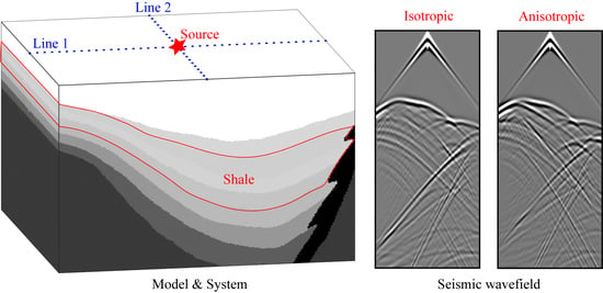
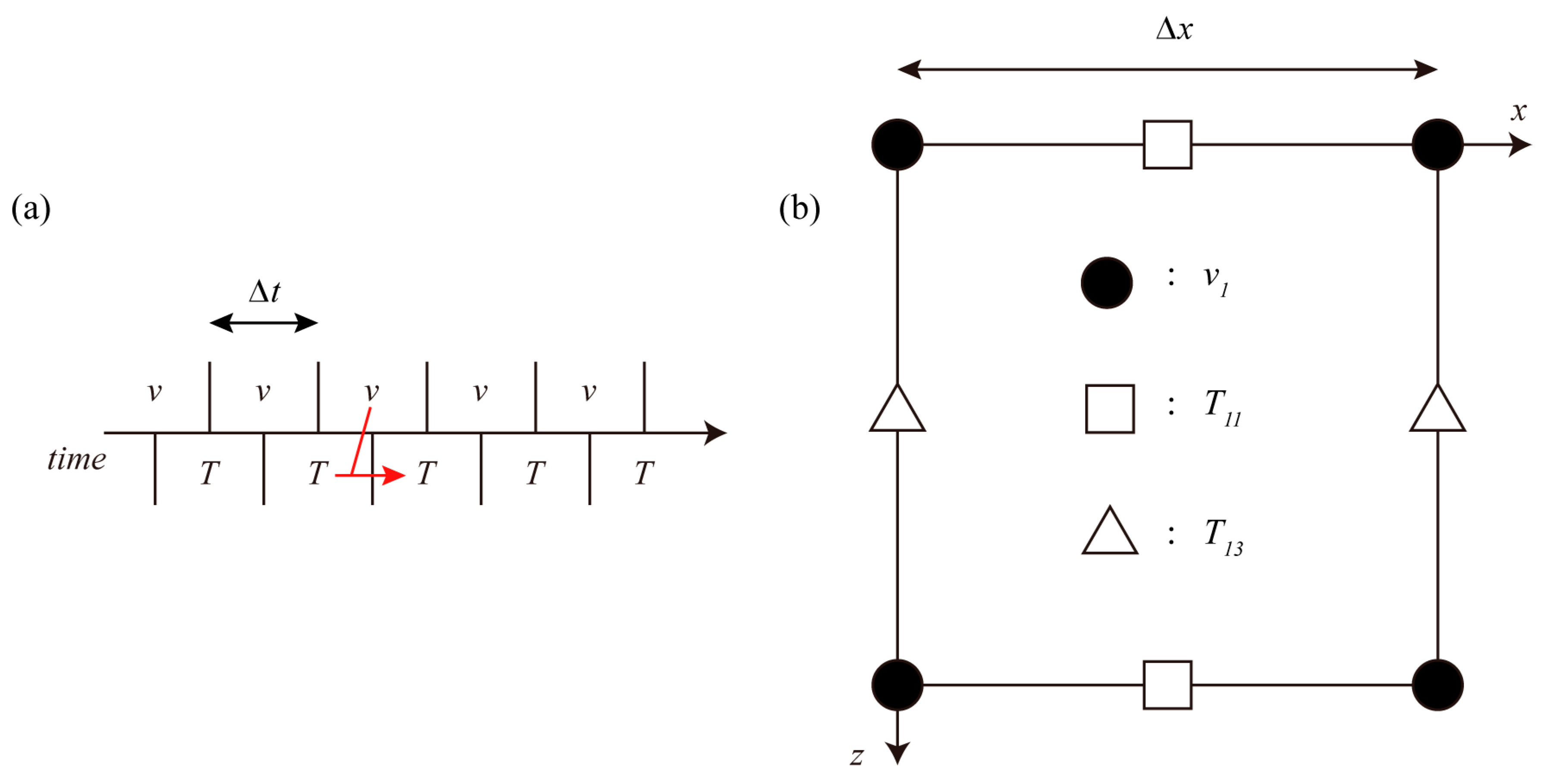
2.1. Forward Modeling for 3D TTI Model

Considering the shale’s strong anisotropy characteristics, the assumption of the isotropic medium is inappropriate, and the adoption of transversely isotropic media is currently recognized as a more reasonable description of shale media [23,24]. In our study, the calculation of the seismic wavefield is based on the elastic wave equation:

$$\rho \frac{{\partial }^2{u}_i}{\partial t^2}=c_{ijkl}\frac{{\partial }^2{u}_k}{\partial x_j\partial x_l}+\rho F_i,$$

(1)

where $u$ represents the particle’s displacement, $\rho$ and $F$ are the medium’s density and the external force, respectively, $c_{ijkl}$ is the stiffness matrix in Hooke’s law and represents the relationship between stress and strain. Considering the symmetry of stress and elastic coefficient tensors, and assuming that the medium is vertical transversely isotropic (VTI), the stiffness matrix $c_{ijkl}$ can be simplified as:

$$\left[\begin{array}{cccccc}{c}_{11}& c_{12}& c_{13}& 0& 0& 0\\ c_{12}& c_{11}& c_{13}& 0& 0& 0\\ c_{13}& c_{13}& c_{33}& 0& 0& 0\\ 0& 0& 0& c_{44}& 0& 0\\ 0& 0& 0& 0& c_{44}& 0\\ 0& 0& 0& 0& 0& c_{66}\end{array}\right],$$

(2)

using the weak anisotropy hypothesis proposed by Thomsen [25], the elastic parameters in (2) can be transformed to:

$$\{\begin{array}{l}\epsilon =\frac{c_{11}-c_{33}}{2c_{33}}, \gamma =\frac{c_{66}-c_{44}}{2c_{44}},\\ v_{p_z}=\sqrt{\frac{c_{33}}{\rho } }, v_{s_z}=\sqrt{\frac{c_{44}}{\rho }},\\ \delta =\frac{{\left(c_{13}+c_{44}\right)}^2-{\left(c_{33}-c_{44}\right)}^2}{2c_{33}\left(c_{33}-c_{44}\right)},\end{array} \{\begin{array}{l}{c}_{11}=\rho \left(1+2\epsilon \right)v_{p_z},\hfill \\ c_{33}=\rho v_{p_z}^2,\hfill \\ c_{44}=\rho v_{s_z}^2,\hfill \\ c_{12}=\rho v_{p_z}^2\left[1+2\epsilon -2\left(1-f^{\prime }\right)\left(1+2\gamma \right)\right],\hfill \\ c_{13}=\rho v_{p_z}^2\sqrt{f^{\prime }\left(f^{\prime }+2\delta \right)}-\rho v_{s_z}^2,\hfill \\ c_{66}=\rho \left(1+2\gamma \right)v_{s_z}^2=0.5\left(c_{11}-c_{12}\right),\hfill \end{array}$$

(3)

where $f^{\prime }=1-v_{s_z}^2/v_{p_z}^2$, $\epsilon$, and $\delta$ represent the difference of P-wave velocity in the direction of vertical, horizontal, and 45°, i.e., the measurement of P-wave anisotropy, $\delta$ represent the anisotropic strength of S-wave, $v_{p_z}$ and $v_{s_z}$ are the velocity of P- and S-wave along the vertical (depth) direction, respectively. From Equations (2) and (3), we can see that for the VTI medium, there are six stiffness parameters and five of them are independent with each other.

Equations (1)–(3) establish the elastic wave forward modeling theory of VTI medium (vertical transversely isotropic, i.e., medium with vertical symmetry axis). For TTI medium (tilted transversely isotropic, i.e., medium with tilted symmetry axis), we can make use of its spatial inclination and perform a coordinate transformation to calculate the seismic wavefield.

In this paper, we use the staggered-grid finite-difference method [21,22,26,27,28,29] to calculate the elastic wave equation. Details of this method are shown in Appendix A. The finite-difference (FD) method is a crucial numerical tool in the modeling of earthquake ground motion, and the staggered-grid FD algorithm is one of the most popular FD schemes and has been proved to be flexible and relatively accurate in the analysis of wave propagation problems [27,29,30]. The staggered-grid FD algorithm computes the pressure at a set of spatial points, and the velocity at another set of spatial points [31]. One of the attractive features of the staggered-grid approach is the velocities are updated independently from the stresses, which allows for a very efficient and concise implementation scheme [27].

2.2. Quantitative Evaluation of the Shale Anisotropy’s Impact

In order to analyze the shale anisotropy’s impact on the seismic wavefield, the comparison between seismic data with and without anisotropy is needed. We use the envelope misfit EM and the phase misfit PM to perform the quantitative evaluation. These two parameters are put forward by Kristek [30] to evaluate both the difference in the amplitude and phase between two signals. Let $S_{REF}\left(t\right)$ be the reference data and $S\left(t\right)$ be the data to be compared, the envelope misfit EM is

$$EM=\frac{\sqrt{{{\displaystyle \sum }}_m{\left[\left|{\widehat{S}}_{REF}\left(t_m\right)\right|-\left|\widehat{S}\left(t_m\right)\right|\right]}^2}}{\sqrt{{{\displaystyle \sum }}_m{\left|{\widehat{S}}_{REF}\left(t_m\right)\right|}^2}}$$

(4)

and the phase misfit PM is

$$PM=\frac{\sqrt{{{\displaystyle \sum }}_m{\left[\left|{\widehat{S}}_{REF}\left(t_m\right)\right|·Arg\left({\widehat{S}}_{REF}\left(t_m\right)/\widehat{S}\left(t_m\right)\right)\right]}^2}}{\pi ·\sqrt{{{\displaystyle \sum }}_m{\left|{\widehat{S}}_{REF}\left(t_m\right)\right|}^2}}$$

(5)

where ${\widehat{S}}_{REF}\left(t\right)$ and $\widehat{S}\left(t\right)$ are the analytical signals of $S_{REF}\left(t\right)$ and $S\left(t\right)$, respectively (an analytical signal is a complex-valued function that has no negative frequency components, its real and imaginary parts are real-valued functions related to each other by the Hilbert transform [32]). $\left|z\right|$ is the modulus of a complex number $z$ and $Arg\left(z\right)$ is the principal value of $z$’s argument. From Equations (4) and (5), it can be seen that the envelope misfit EM and the phase misfit PM are the relative average errors of two waveforms. If the value of EM is 1, it means that the average amplitude difference between the two signals is doubled. For PM, if its value is 1, the polarities of all seismic phases in two signals are completely opposite.

In this paper, we use the following steps (Figure 1) to quantitatively evaluate the impact of shale anisotropy on seismic wavefield:

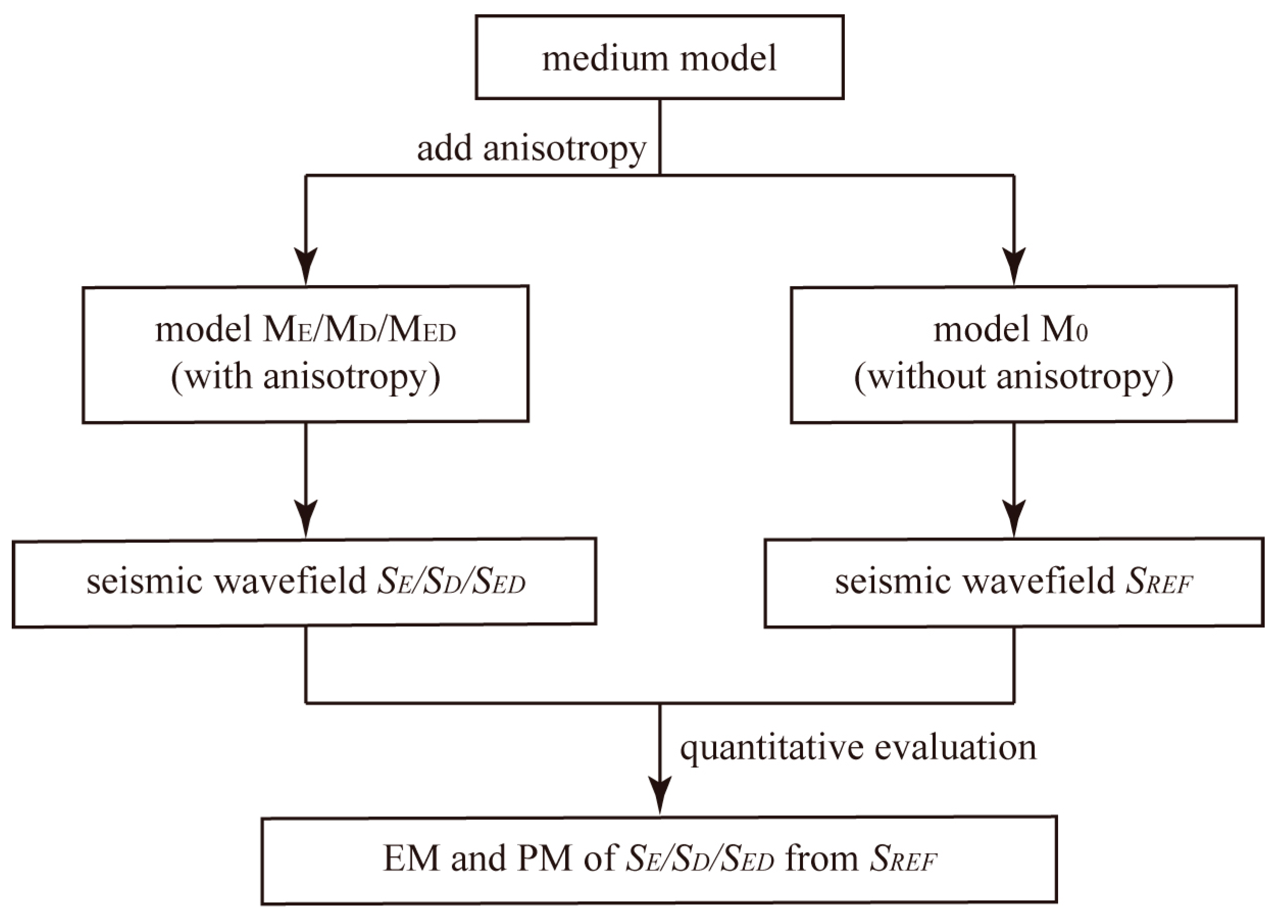
• Set the parametric medium model M₀ (without anisotropy) according to the geological characteristics of shale reservoirs or the actual oilfield models. Add three sets of different anisotropic parameters to the shale layer of model M₀ and establish three different medium models with shale anisotropy, i.e., M_E ($\epsilon$ = 0.25, $\delta$ = 0), M_D ($\epsilon$ = 0, $\delta$ = 0.25), and M_ED ($\epsilon$ = 0.25, $\delta$ = 0.25). The parameters of model M_ED are reasonably geologically chosen from several shale anisotropy studies in China ([9,17]), while the other two models (M_E and M_D) are built based on the variable-controlling approach, for the purpose of exploring the impact of different anisotropy parameters;
• Use the forward modeling method to calculate the elastic wavefields of four medium models ($S_{REF}$ for model M₀, $S_E$ for model M_E, $S_D$ for model M_D, and $S_{ED}$ for model M_ED);
• Compare the seismic wavefields with each other and calculate the envelope misfit EM and the phase misfit PM of the wavefield $S_E$/$S_D$/$S_{ED}$ from $S_{REF}$. Evaluate the impact of shale anisotropy on elastic seismic wave response.

3. Evaluation of Simulation Models

In this section, we set two synthetic models of different complexity and used our method to evaluate the impact of anisotropy on their seismic wavefield. Based on the geological sedimentary characteristics of actual shale strata, we set two models, i.e., the horizontal layered VTI model and the curved layered TTI model.

3.1. Horizontal Layered VTI Model

3.1.1. Parameters and Wavefield Data

The horizontal layered VTI model, seismic source, and observation system are shown in Figure 2. This model has three layers and the shale reservoir is located in the middle. Details of each layer’s parameters are shown in

Table 1. Media parameters for multi-layered VTI model.

Layer	Depth (m)	VP (m/s)	VS (m/s)	Density (g/cm3)
1	0~800	3000	1700	2.0
2	800~1500	3500	2000	2.3
3	1500~2000	4000	2300	2.4

. An explosion source is situated in the center of the surface (1000, 1000, 0 m) with the Ricker wavelet time function (20 Hz). There are two crossing survey lines distributed along the X direction and the Y direction, respectively, each with 201 geophones and 10 m spacing. The grid number is 201 × 201 × 201 (X/Y/Z) with the spatial spacing 10 m and the time sampling interval is 0.5 ms. According to the steps in Section 2.2 (Figure 1), the horizontal layered VTI model in Figure 2 is set as model M₀ (without anisotropy). We added three groups of anisotropic parameters to the shale layer and built up three different anisotropic models, i.e., M_E ($\epsilon$ = 0.25, $\delta$ = 0), M_D ($\epsilon$ = 0, $\delta$ = 0.25), and M_ED ($\epsilon$ = 0.25, $\delta$ = 0.25).

For models M₀/M_E/M_D/M_ED, the seismic waveform records of 402 geophones are respectively synthesized ($S_{REF}/S_E$/$S_D$/$S_{ED}$). The three-component waveforms of model M₀, namely $S_{REF}$, is shown in Figure 3a–c. Comparing the X-, Y-, and Z-component waveforms of each detector, we can see that the X- and Y-component records of the two survey lines (line 1: No.1~201 and line 2: No.202~402) are different, while the Z-component records are entirely consistent. The reason for this is that the horizontal coordinates of the two survey lines are different (line 1 is arranged along the X direction, and line 2 is along the Y direction). Therefore, for an explosive seismic source, the received X- and Y-waveforms are different, while the Z-component records of two lines are the same, because the symmetry axis of the medium is along the vertical direction (VTI medium).

Considering that surface seismic exploration usually uses a single-component (generally Z-component) detector, our study mainly focuses on analyzing the influence of shale anisotropy on the Z-component waveforms. It can be seen from Figure 3c that the Z-component wavefield has four strong phases. Based on the analysis in Figure 3d, these four phases respectively correspond to direct P wave, reflected P-P wave, reflected P-SV wave, and P-P-P-P wave.

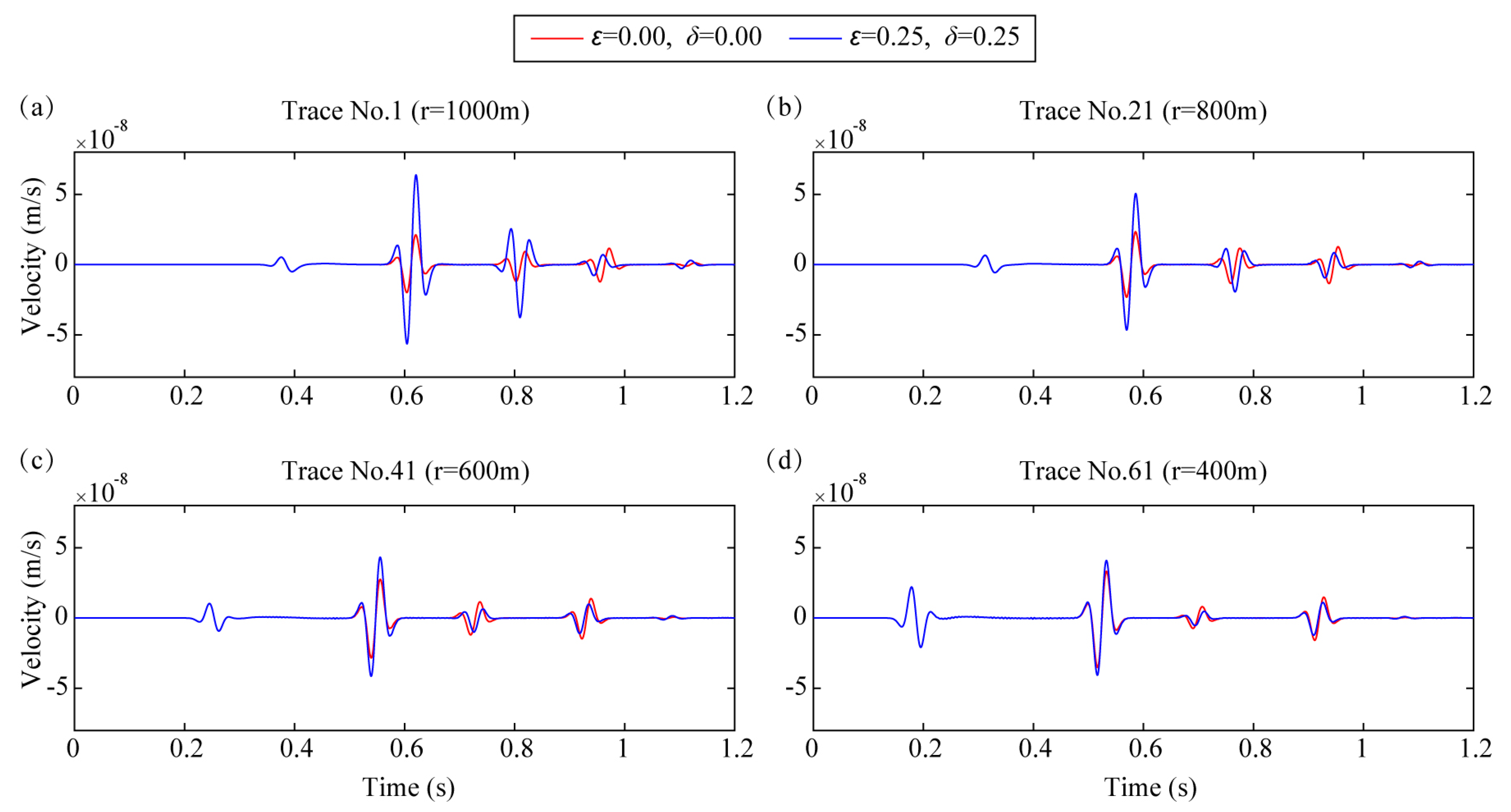
3.1.2. Effect of Anisotropy on Different Seismic Phases

Seismic waves with different phases (direct P/S, reflected, or transmitted wave) propagate in different paths, so the impact of shale anisotropy on them may also be different. Figure 4 shows the comparison of waveforms from model M_ED ($\epsilon$ = 0.25, $\delta$ = 0.25) and M₀ ($\epsilon$ = 0, $\delta$ = 0).

From Figure 4, we can find that for each detector:

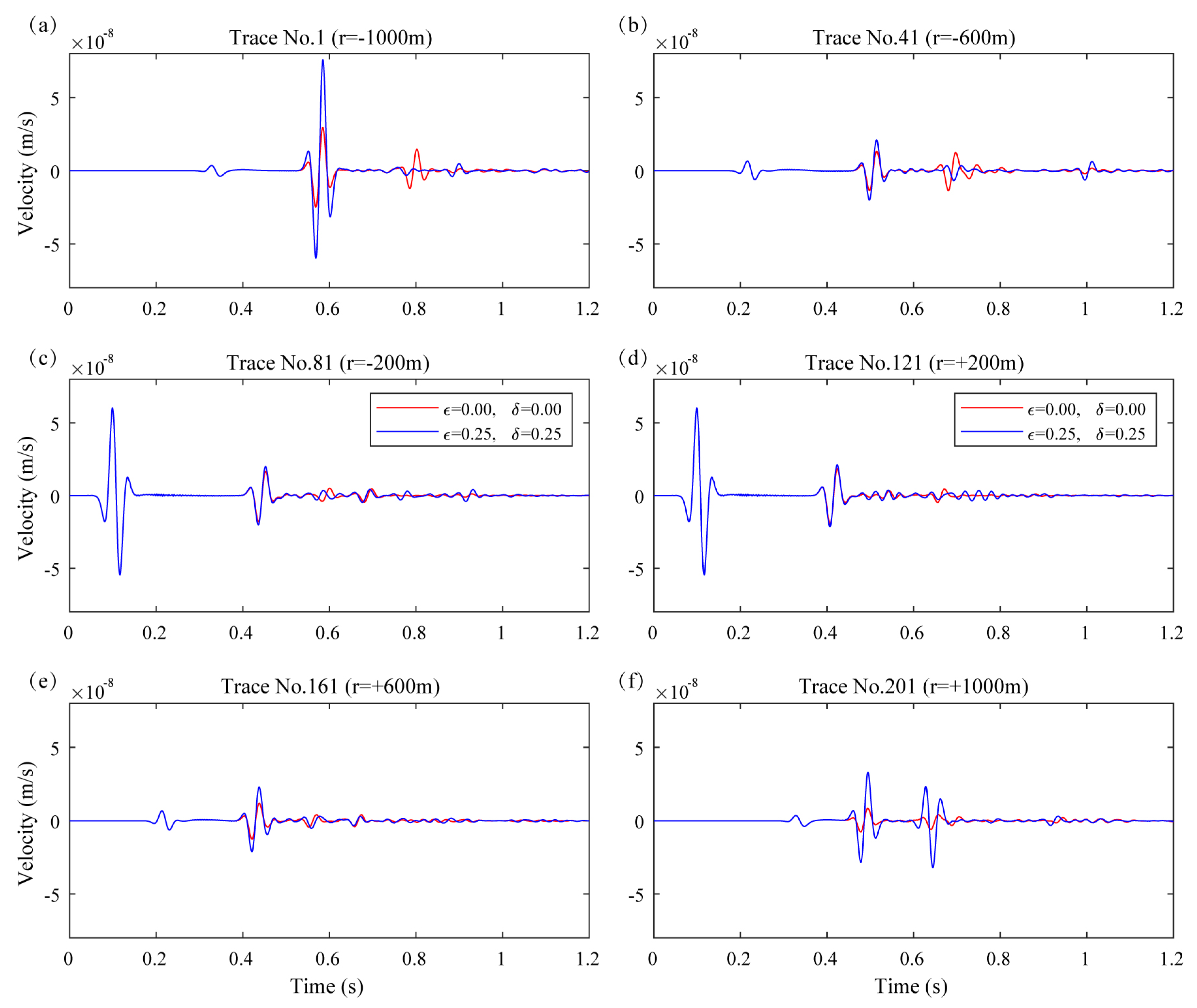
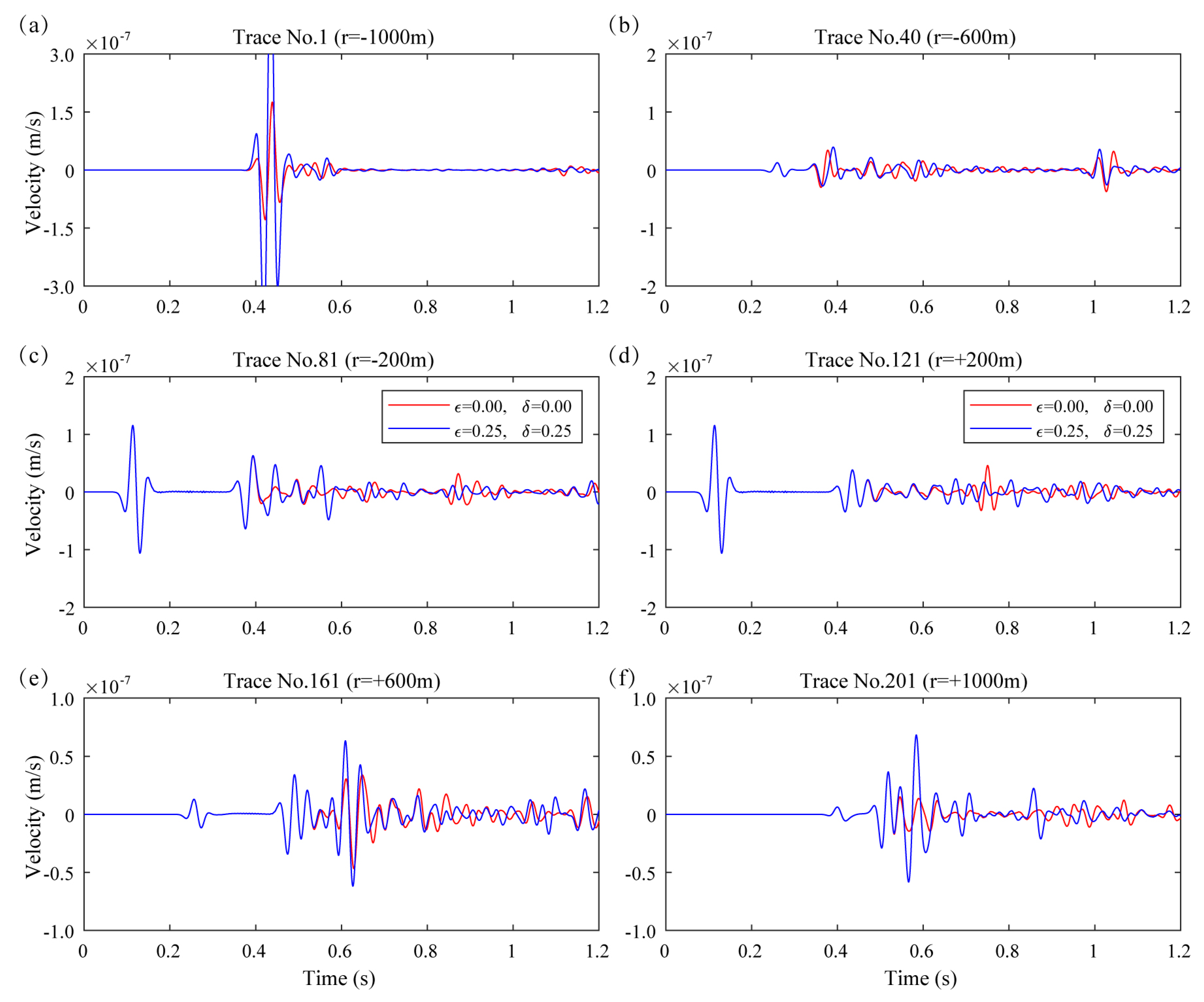
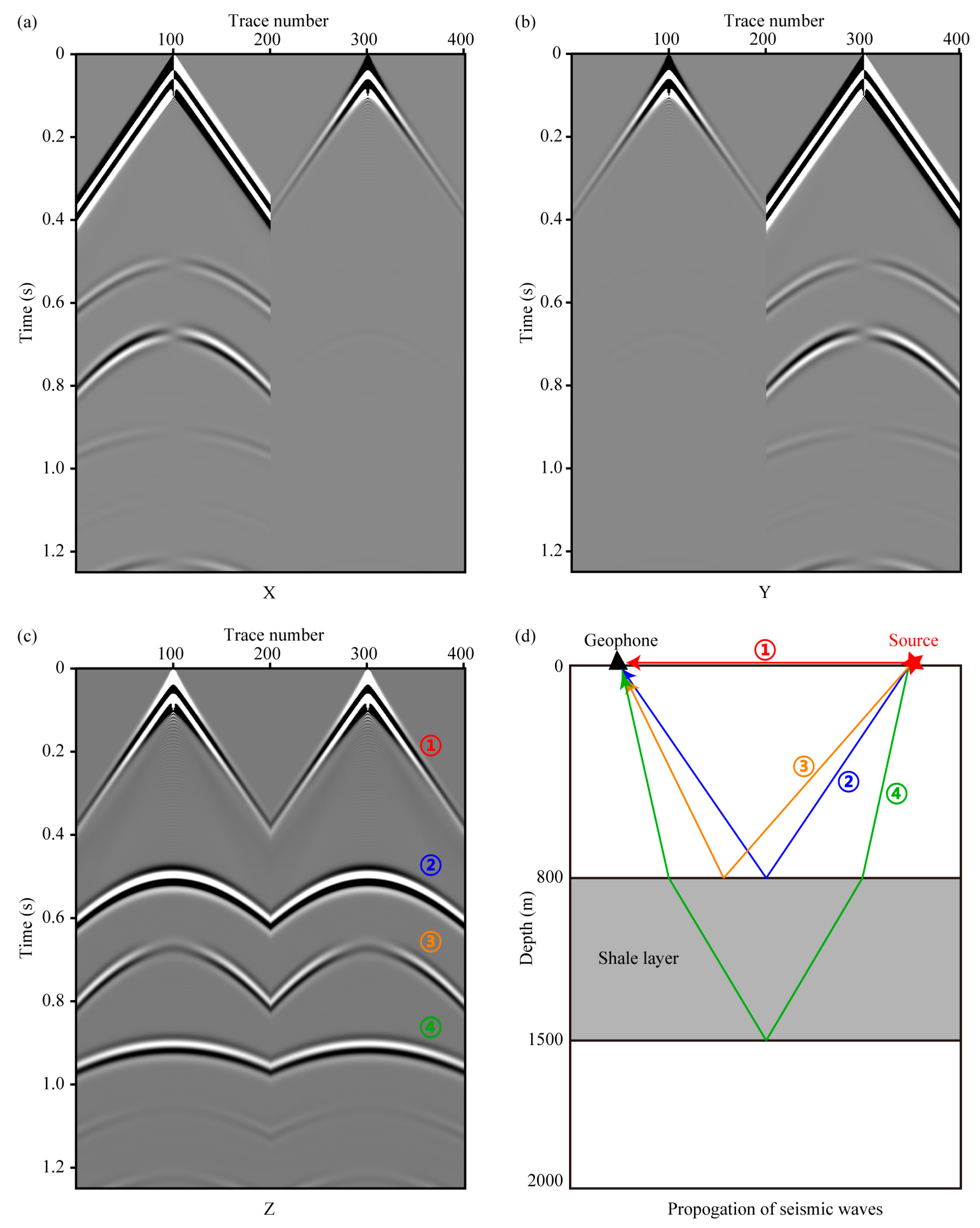
• Direct P wave. The first seismic phases (direct P wave) of two models are exactly the same. From its propagation path (Figure 3d), we can see that the direct P wave traveled from the seismic source to the detector through the surface, so it is not affected by the shale anisotropy.
• Transmitted and reflected P-P-P-P wave. The fourth seismic phases (P-P-P-P wave, its propagation path is shown in Figure 3d) are totally different. When adding anisotropy to the shale layer, the velocities of P-waves along different directions propagating in it are changed and not the same. So this seismic wave’s arrival time, amplitude and phase are all influenced by shale anisotropy.
• Reflected P-P wave and P-SV wave. The arrival time of the second and third phases (reflected P-P and P-SV waves, their paths are shown in Figure 3d) is the same, while their amplitudes are different. The reasons for this are probably because:
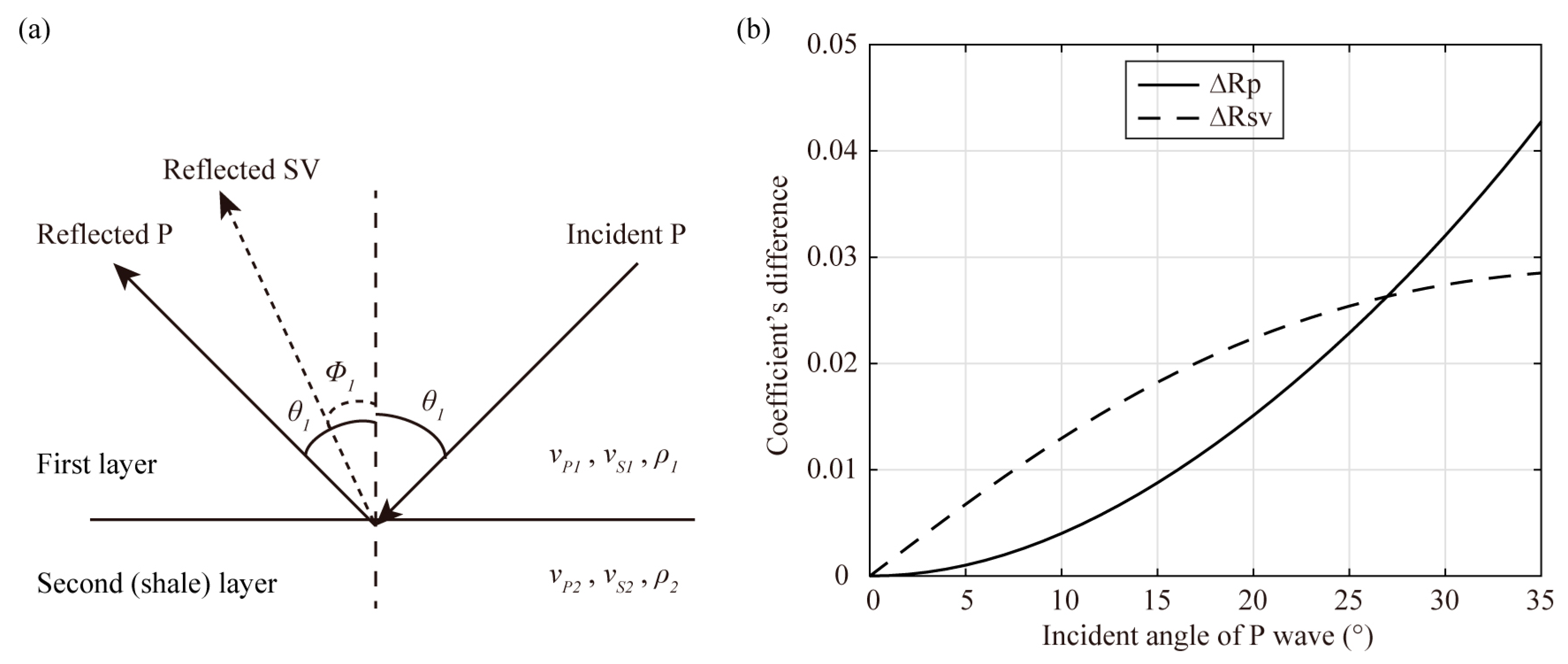
  • Arrival time. These two waves are both reflected at the interface of the first layer and the shale layer. The first layer is isotropic, so we can use the Snell’s law to analyze the reflection:

    $$\frac{v_{P1}}{\sin {\theta }_1}=\frac{v_{S1}}{\sin {\varphi }_1},$$

    (6)

    where $v_{P1}$ is the velocity of incident P-wave (same as the reflected P-wave’s velocity) and $v_{S1}$ is the reflected SV-wave’s velocity at the interface, respectively, ${\theta }_1$ and ${\varphi }_1$ are the corresponding angles (Figure 5a). When we added anisotropy to the shale layer, velocities of P and S wave in the first layer are not changed, so $v_{P1}$ and $v_{S1}$ remain unchanged. From Equation (6), we can find that ${\theta }_1$, ${\theta }_2$, and the propagation paths are not influenced by anisotropy, so is the arrival time.
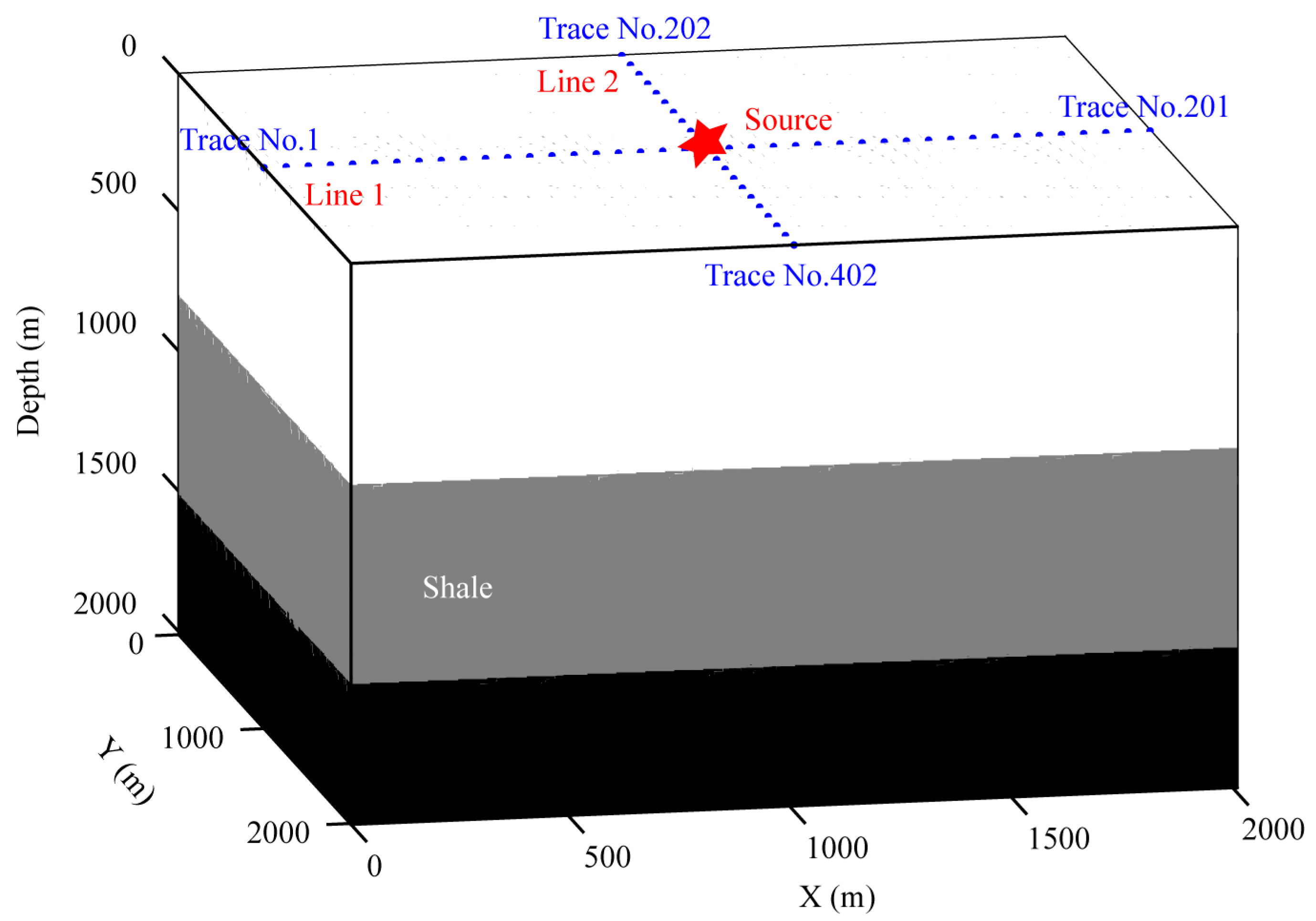
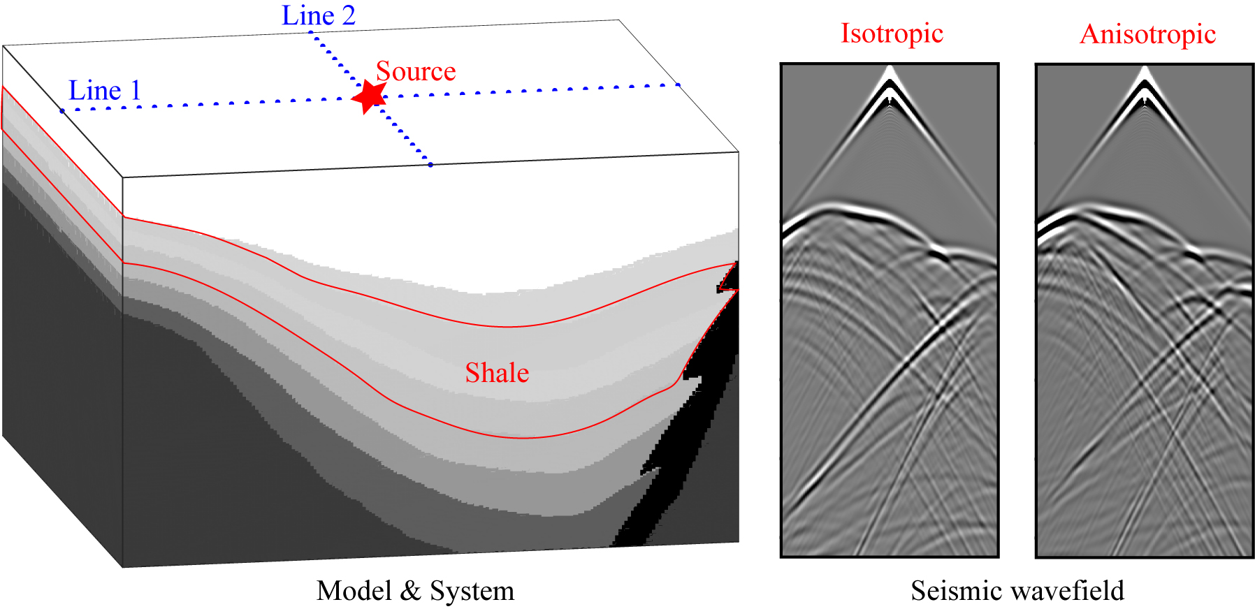
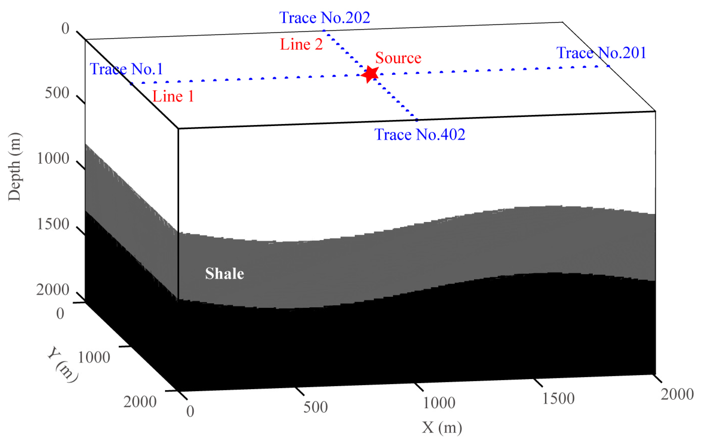
  • Amplitude. The amplitude of reflected P and SV waves can be evaluated using the anisotropic reflectivity and transmissivity calculator code by Malehmir and Schmitt [19]. According to the observation system and source location (Figure 2), the maximum incident angle ${\theta }_1$ of P wave between the first and second (shale) layer is about 32°. Then, we set ${\theta }_1$ from 0 to 35° and calculate the reflection coefficients of reflected P and SV waves. The differences of reflection coefficients with and without anisotropy are shown in Figure 5b. We can find that when adding anisotropy to the VTI model (Figure 2), the reflection coefficients of reflected P and SV waves are both changed. Considering that the propagation paths of these two waves are unchanged, so the Z-component amplitudes of reflected P-P and P-SV waves are influenced by the shale anisotropy.

3.1.3. Amplitude and Phase Misfit by Anisotropy

Using the forward modeling method in Section 2.1, we synthesized the seismic waveforms of the four medium models M₀/M_E/M_D/M_ED ($\epsilon /\delta$ are 0/0, 0.25/0, 0/0.25, and 0.25/0.25). Based on Equations (4) and (5), we calculated the wavefields’ amplitude deviation EM and phase deviation PM of the anisotropic model M_E/M_D/M_ED from the model M₀ (without anisotropy). The results are shown in Figure 6. Here, the normalized epicentral distance (i.e., epicentral distance divided by wavelength) is used. From Figure 6, we can see the following points:

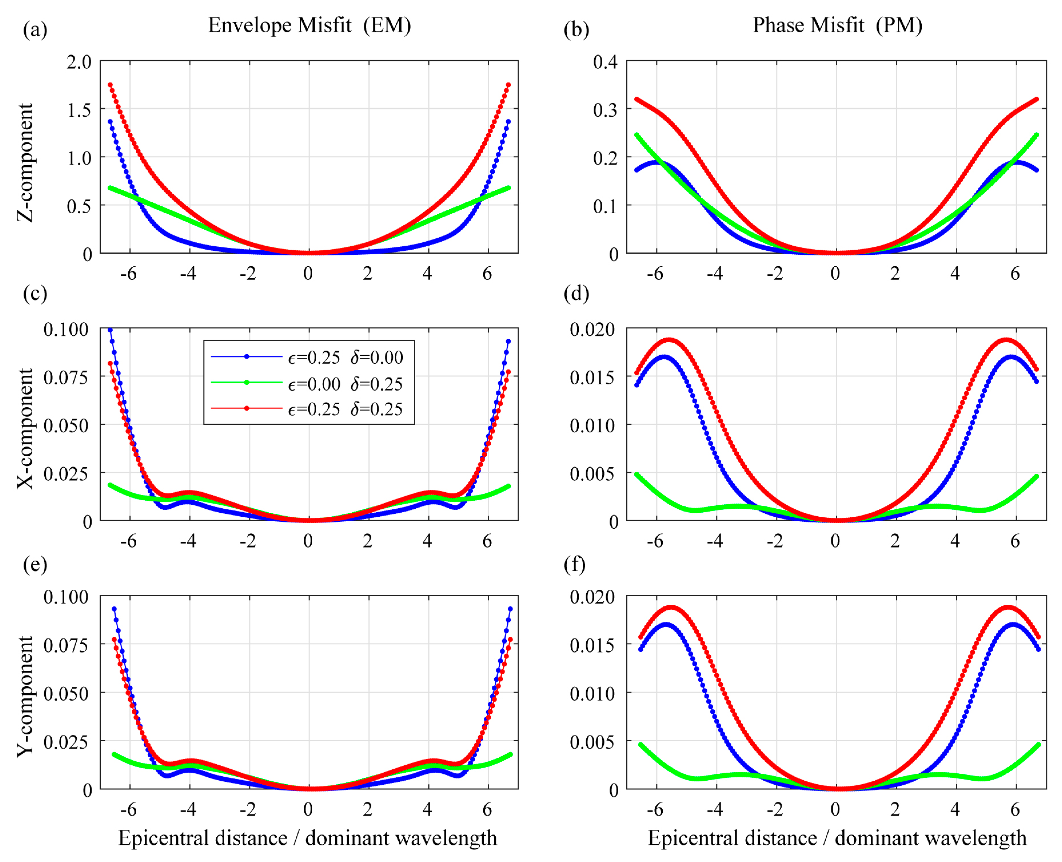
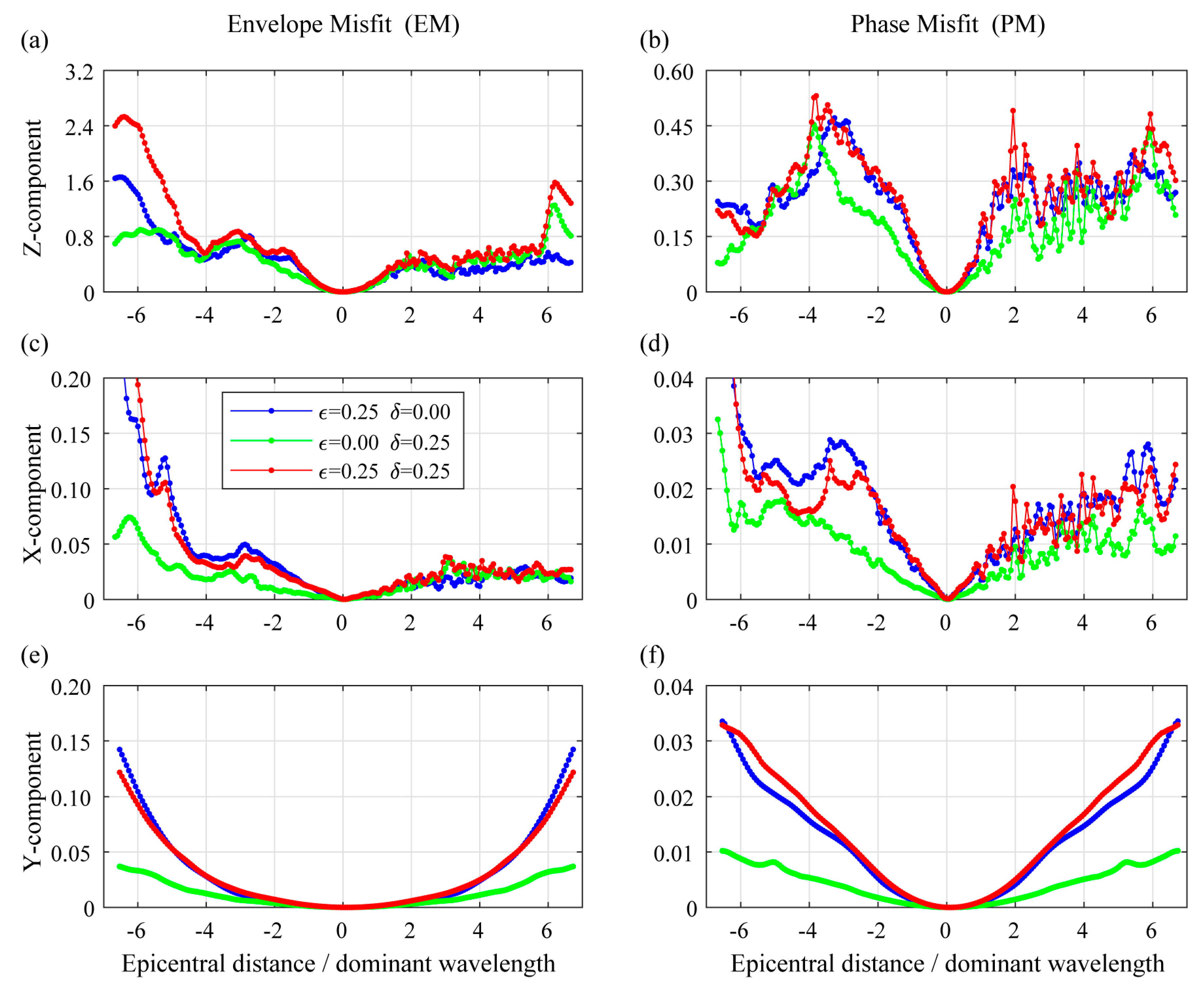
• The amplitude deviation EM and phase deviation PM of the two survey lines in Z-component are significantly larger than their X- and Y-components, which indicates that anisotropy has a more significant influence on the vertical component. It is speculated that the reason may be that the propagation distance of the seismic wave in the vertical direction is larger than that in the horizontal direction and the medium model’s symmetric axis is along the vertical direction.
• The maximum EM of the two survey lines in Z-component is greater than 1, which indicates that the waveform’s amplitude will be significantly affected by the shale anisotropy. In actual seismic exploration, the amplitude is of great importance to the inversion of reservoir parameters, so ignoring anisotropy may lead to errors in reservoir characterization.
• The Z-component phase deviation PM of the two survey lines reaches 0.4. As is mentioned above, if PM is 1, the polarities of the two signals are completely opposite. So this means that the waveforms’ phase morphology is also largely changed due to anisotropy. The inaccurate phase may lead to the low resolution of migration imaging results, which also affects the processing and interpretation of actual exploration seismic data.
• The amplitude deviation EM and phase deviation PM of X/Y/Z components on two sides of the source are symmetrical, which is caused by the symmetry axis’s verticality of the VTI model. Moreover, the EM all increases with the increase of epicentral distance (offset), while the PM increases first and then decreases. This may because the maximum value of the difference in phase is the odd multiples of π. Therefore, if the phase’s difference gradually increases from 0 to 2π, the difference in waveform’s phase will become bigger first and then smaller, and the calculated PM will also increase first and then decrease correspondingly.
• In most of the results, the deviations of the model M_ED ($\epsilon$ = 0.25, $\delta$ = 0.25) are relatively larger than the other two models M_E ($\epsilon$ = 0.25, $\delta$ = 0) and M_D ($\epsilon$ = 0, $\delta$ = 0.25).

3.2. Curved Layered TTI Model

In this section, we analyzed shale anisotropy’s impact on the seismic wavefield of a curved multi-layer TTI model [28]. The geometry of the medium model, source, and observation system is shown in Figure 7. Parameters for the wavefields’ forward modeling are the same as Section 3.1. Details of each layer’s parameters are listed in

Table 2. Media parameters for multi-layered TTI model.

Layer	Depth (m)	Thickness (m)	VP (m/s)	VS (m/s)	Density (g/cm3)
1	0	700–900	3000	1700	2.0
2	800	500	3500	2000	2.3
3	1500	600–800	4000	2300	2.4

and the shale reservoir is located in the middle. The dip angle of TTI media’s symmetry axis is 40° and the azimuth angle is 0°. Similar to Section 3.1, when anisotropic parameters are added to the shale layer, four models are respectively set: M₀ ($\epsilon$ = 0, $\delta$ = 0), M_E ($\epsilon$ = 0.25, $\delta$ = 0), M_D ($\epsilon$ = 0, $\delta$ = 0.25), and M_ED ($\epsilon$ = 0.25, $\delta$ = 0.25).

The seismic waveform records of 402 geophones are respectively forward synthesized for four models M₀, M_E, M_D, and M_ED. The comparison of Z-component wavefields with and without anisotropy in the first survey line (geophone No.1–No.201) is shown in Figure 8, and the waveforms of eight different epicentral distance detectors (−1000/−600/−200/+200/+400/+1000 m, the positive and the negative sign indicate that the detectors are on left and right sides of the seismic source, respectively) are shown in Figure 9. From Figure 8 and Figure 9, it can be seen that before and after anisotropy is added, except the direct P wave is not affected, the subsequent phases are all affected by different degrees. When adding shale anisotropy, the amplitude of reflected P-P wave (the second phase) is increased. The arrival time, phase, and amplitude of the other phases (P-SV, P-P-P-P, multiple waves, etc.) are all changed due to the shale anisotropy.

Similar as Section 3.1, using Equations (4) and (5), we calculated the seismic wavefields’ amplitude deviation (envelope misfit EM) and phase deviation (phase misfit PM) of the anisotropic model M_E/M_D/M_ED ($\epsilon$/$\delta$ are 0.25/0, 0/0.25, 0.25/0.25) from the model M₀ (without anisotropy). The results are shown in Figure 10. Here, the deviation results of Z- and X-component are from line 1, while the results of Y-component are from line 2. From Figure 10, we can find that:

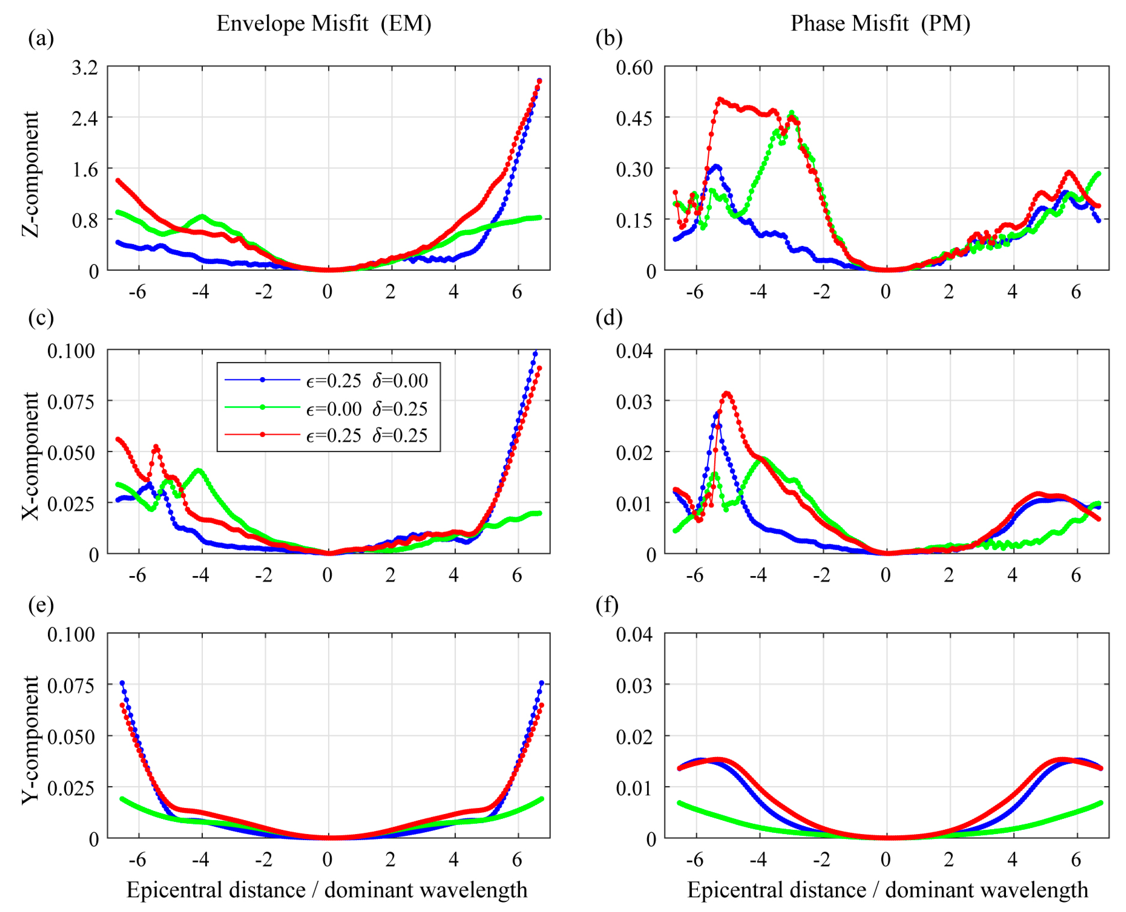
• Same as the VTI model, the EM and PM of Z-component are still larger than that of X- and Y- components. The maximum EM is still greater than one, and the maximum PM is about 0.5 (relatively large; if PM is 1, the polarities of all phases of the two signals are entirely opposite).
• Unlike the VTI model, with the increase of epicentral distance, the variation trend of EM and PM are complicated. Moreover, the EM and PM of Y-component are symmetrical, while the X- and Z- components are not. The reasons are probably because the shape and structure of TTI model are complex, and its symmetry axis is not along the vertical direction. These phenomena prove that the impact of shale anisotropy relies heavily on the model.
• In most of the results, the deviations of models M_ED, M_E, and M_D from M₀ are close to each other. This indicates that the impact of different anisotropic parameters on the wavefield is complicated in the curved TTI model, and the influence strength of each parameter cannot be determined simply as the horizontal layered VTI model.

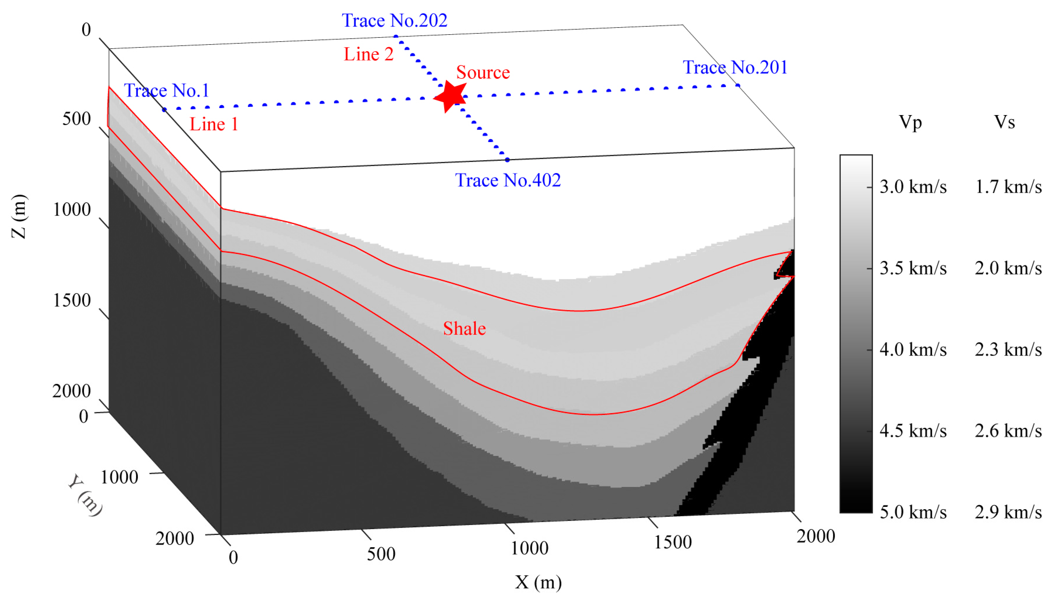
4. Evaluation of JY Depression Model

Through the analysis of the simulation VTI and TTI model, we find that if the medium model is complex (shape is distorted and the symmetry axis is inclined), the influence of shale anisotropy on wavefield is complicated and requires specific analysis. In this section, we try to apply the established evaluation method (Figure 1) to quantitatively analyze the anisotropic influence of an actual shale model (Jiyang depression model) in eastern China from China Petrochemical Corporation (Sinopec).

Figure 11 shows the geometry and velocity parameters of the 3D JY (Jiyang) depression model, and the location of the seismic source and two survey lines (with 402 geophones). When setting the JY depression model, we did some compression along the X direction and conducted continuation modeling along the Y direction. The shale layer (red) is located in the middle and we add four groups of different anisotropic parameters to it, thus set four models, i.e., M₀ ($\epsilon$ = 0, $\delta$ = 0), M_E ($\epsilon$ = 0.25, $\delta$ = 0), M_D ($\epsilon$ = 0, $\delta$ = 0.25), and M_ED ($\epsilon$ = 0.25, $\delta$ = 0.25). The grid number of the model is 201 × 201 × 201 with spatial size 10 × 10 × 10 m and the time sampling interval is 0.5 ms. The explosive source is located in the center of the surface (1000, 1000, 0 m) and the source time function is Ricker wavelet (20 Hz).

For four models (M₀/M_E/M_D/M_ED, with different shale anisotropy), the seismic waveform records of each detector are forward simulated, respectively. Figure 12 shows the comparison of the Z-component wavefield of line 1 (trace numbers No.1–No.201, Figure 11) with and without the shale anisotropy. Figure 13 illustrates the comparison of Z-component waveforms of eight detectors (with different epicentral distances).

Since the shape and structure of the JY model are very complex, it is difficult to analyze the impact of each seismic phase accurately. However, from Figure 12 and Figure 13, we can clearly see that when anisotropy is added, in addition to the direct wave, the subsequent seismic phases are all affected and changed. Moreover, comparing the waveforms of detectors on the left and right side of the seismic source (located at trace No.101), it can be seen that their waveforms are not symmetrical and are affected by different degrees.

After the forward modeling of the JY Depression model, similar to Section 3.1 and Section 3.2, we analyzed the waveforms’ EM and PM of the anisotropic model M_E/M_D/M_ED from the model M₀ (without anisotropy). Figure 14 illustrates the calculation results. Here, the deviation results of Z- and X- components are still from the first survey line, while the Y-component results are from the second survey line (Figure 11). From Figure 14, we can find that:

• Similar to VTI and TTI model, the EM and PM of Z-component are still significantly larger than those of the X- and Y- horizontal components. The maximum EM is greater than one and the maximum PM reaches up to 0.5, which indicates that the impacts of anisotropy on the amplitude and phase are remarkable.
• Unlike the VTI and TTI model, for the JY model, the variation of EM and PM in the X- and Z-component with the epicentral distance (offset) is complicated, while the EM and PM of Y-component gets bigger with the increase of the epicentral distance.
• Same as TTI model but different from VTI model, for the JY model, the deviations of M_ED ($\epsilon$ = 0.25, $\delta$ = 0.25)/M_E ($\epsilon$ = 0.25, $\delta$ = 0)/M_D ($\epsilon$ = 0, $\delta$ = 0.25) are close to each other. This illustrates that the impact of different anisotropic parameters on the wavefield is complicated and needs further study.

5. Discussion and Conclusions

In order to study the impact of shale anisotropy on the seismic wavefield, we proposed a new quantitative evaluation method to calculate the waveform deviations of the anisotropic model from the regular model (without anisotropy). Based on the 3D elastic wave equation and the staggered-grid finite-difference method, the forward modeling theory of the three-component seismic wavefield considering the shale anisotropy was established. Then, we used the envelope misfit (EM) and the phase misfit (PM) to illustrate the differences in waveforms’ amplitude and phase morphology caused by anisotropy. Finally, by comparing the waveforms of the models with/without anisotropy and calculating their EM and PM, we can quantitatively evaluate the impact of shale anisotropy on the seismic wavefield.

We applied the proposed method to analyze the anisotropy’s effect on two simulation models (horizontal layered VTI model and curved layered TTI model) and one actual oilfield model (JY depression model). Tests on simulation and oilfield models prove that the proposed evaluation method is valid and efficient. Moreover, we gained some new cognitions about the anisotropy’s effects. (1) The amplitude and phase deviations caused by anisotropy are significant, with EM lager than 1 and PM up to 0.5. Considering that the EM and PM are the relative deviations of two signals, this means that the shale anisotropy may cause the waveforms’ amplitudes and phase shapes to be affected by a relatively high level. (2) Anisotropy’s impacts on seismic waveform’s vertical and horizontal components are different. In most cases, seismic surveys at the surface use the single-component (Z-component) detectors, so during the data interpretation, the Z-component records are adopted. We found that for these three different models, the anisotropy’s effect on the Z-component is larger than the other X/Y components. (3) The impact of anisotropy on each detector depends on its offset from the source. When the geophones are set at the surface, for the horizontal layered VTI model, as the offset increases, the EM increases while the PM increases first then decreases. Moreover, the anisotropy’s effects on two sides of the seismic source are symmetrical. However, for the curved layered TTI model and JY depression model, the variation trend is not clear. This illustrates that the anisotropy’s impact relies heavily on the structure and symmetry axis of the medium model. (4) The influences of different anisotropy parameters on seismic wavefield are different. Based on the variable-controlling approach, we set three different anisotropic models (M_E/M_D/M_ED, whose $\epsilon /\delta$ are 0.25/0, 0/0.25, and 0.25/0.25, respectively). For the VTI model, the deviations of M_ED from M₀ (without anisotropy) are the largest, while for the other two models (TTI and JY model), the deviations of M_E/M_D/M_ED are about at the same level.

According to our research, the impact of shale anisotropy on seismic wavefield is complicated and cannot be simply judged. So, for a particular oilfield model, we need specific analysis. The proposed method provides a useful and quantitative tool for anisotropy’s evaluation. Furthermore, by using this method and calculating the waveform misfits from the actual seismic data, we can evaluate the accuracy of different anisotropic models and find the most suitable model for seismic data interpretation. Based on this idea, the anisotropic parameters inversion can be performed by seeking the minimum deviations between the synthetic and the actual seismic wavefield data. Moreover, as detectors with different offsets are affected differently, we can identify the observation area where the detectors are less affected by the shale anisotropy, then use the traditional interpretation method to process the selected wavefield data, so as to improve the accuracy and reliability of sweet spots prediction and reservoir characterization.

References

1. Zahid, S.; Bhatti, A.A.; Ahmad Khan, H.; Ahmad, T. Development of Unconventional Gas Resources: Stimulation Perspective. In Proceedings of the Production and Operations Symposium, Oklahoma City, OK, USA, 31 March–3 April 2007; Society of Petroleum Engineers: Dallas, TX, USA, 2007. [Google Scholar]
2. Jia, C.; Zheng, M.; Zhang, Y. Unconventional hydrocarbon resources in China and the prospect of exploration and development. Pet. Explor. Dev. 2012, 39, 139–146. [Google Scholar] [CrossRef]
3. Stark, P.H.; Chew, K.; Fryklund, B. The role of unconventional hydrocarbon resources in shaping the energy future. In Proceedings of the IPTC 2007 International Petroleum Technology Conference, Dubai, UAE, 4–6 December 2007; Volume 3, pp. 1876–1881. [Google Scholar]
4. Prasad, M.; Pal-Bathija, A.; Johnston, M.; Rydzy, M.; Batzle, M. Rock physics of the unconventional. Lead. Edge 2009, 28, 34–38. [Google Scholar] [CrossRef]
5. Vernik, L.; Nur, A. Ultrasonic velocity and anisotropy of hydrocarbon source rocks. Geophysics 1992, 57, 727–735. [Google Scholar] [CrossRef]
6. Johnston, J.E.; Christensen, N.I. Seismic anisotropy of shales. J. Geophys. Res. Solid Earth 1995, 100, 5991–6003. [Google Scholar] [CrossRef]
7. Grechka, V.; Yaskevich, S. Azimuthal anisotropy in microseismic monitoring: A Bakken case study. Geophysics 2014, 79, KS1–KS12. [Google Scholar] [CrossRef]
8. Ong, O.N.; Schmitt, D.R.; Kofman, R.S.; Haug, K. Static and dynamic pressure sensitivity anisotropy of a calcareous shale. Geophys. Prospect. 2016, 64, 875–897. [Google Scholar] [CrossRef]
9. Liu, X.-W.; Guo, Z.-Q.; Liu, C.; Liu, Y.-W. Anisotropy rock physics model for the Longmaxi shale gas reservoir, Sichuan Basin, China. Appl. Geophys. 2017, 14, 21–30. [Google Scholar] [CrossRef]
10. Wang, Y.; Li, C.H. Investigation of the P- and S-wave velocity anisotropy of a Longmaxi formation shale by real-time ultrasonic and mechanical experiments under uniaxial deformation. J. Pet. Sci. Eng. 2017, 158, 253–267. [Google Scholar] [CrossRef]
11. Zhang, F.; Li, X.; Qian, K. Estimation of anisotropy parameters for shale based on an improved rock physics model, part 1: Theory. J. Geophys. Eng. 2017, 14, 143–158. [Google Scholar] [CrossRef]
12. Zhang, Y.Y.; Jin, Z.J.; Chen, Y.Q.; Liu, X.W.; Han, L.; Jin, W.J. Pre-stack seismic density inversion in marine shale reservoirs in the southern Jiaoshiba area, Sichuan Basin, China. Pet. Sci. 2018, 15, 484–497. [Google Scholar] [CrossRef]
13. Carcione, J.M.; Helle, H.B.; Zhao, T. Effects of attenuation and anisotropy on reflection amplitude versus offset. Geophysics 1998, 63, 1652–1658. [Google Scholar] [CrossRef]
14. King, A.; Talebi, S. Anisotropy Effects on Microseismic Event Location. Pure Appl. Geophys. 2007, 164, 2141–2156. [Google Scholar] [CrossRef]
15. Warpinski, N.R.; Waltman, C.K.; Du, J.; Ma, Q. Anisotropy Effects in Microseismic Monitoring. In Proceedings of the SPE Annual Technical Conference and Exhibition, New Orleans, LA, USA, 4–7 October 2009; Society of Petroleum Engineers: Dallas, TX, USA, 2009. [Google Scholar]
16. Tsvankin, I.; Gaiser, J.; Grechka, V.; van der Baan, M.; Thomsen, L. Seismic anisotropy in exploration and reservoir characterization: An overview. Geophysics 2010, 75, 75A15–75A29. [Google Scholar] [CrossRef]
17. Sun, W.; Fu, L.; Guan, X.; Wei, W. A study on anisotropy of shale using seismic forward modeling in shale gas exploration. Chin. J. Geophys. 2013, 56, 961–970. [Google Scholar]
18. Meléndez-Martínez, J.; Schmitt, D.R. A comparative study of the anisotropic dynamic and static elastic moduli of unconventional reservoir shales: Implication for geomechanical investigations. Geophysics 2016, 81, D253–D269. [Google Scholar] [CrossRef]
19. Malehmir, R.; Schmitt, D.R. ARTc: Anisotropic reflectivity and transmissivity calculator. Comput. Geosci. 2016, 93, 114–126. [Google Scholar] [CrossRef]
20. Malehmir, R.; Schmitt, D.R. Acoustic Reflectivity From Variously Oriented Orthorhombic Media: Analogies to Seismic Responses From a Fractured Anisotropic Crust. J. Geophys. Res. Solid Earth 2017, 122, 10069–10085. [Google Scholar] [CrossRef]
21. Virieux, J. SH-wave propagation in heterogeneous media: Velocity-stress finite-difference method. Geophysics 1984, 49, 1933–1942. [Google Scholar] [CrossRef]
22. Virieux, J. P-SV wave propagation in heterogeneous media: Velocity-stress finite-difference method. Geophysics 1986, 51, 889–901. [Google Scholar] [CrossRef]
23. Qin, Y.; Zhang, Z.; Li, S. CDP mapping in tilted transversely isotropic (TTI) media. Part I: Method and effectiveness. Geophys. Prospect. 2003, 51, 315–324. [Google Scholar]
24. Guo, P.; McMechan, G.A. Sensitivity of 3D 3C synthetic seismograms to anisotropic attenuation and velocity in reservoir models. Geophysics 2017, 82, T79–T95. [Google Scholar] [CrossRef]
25. Thomsen, L. Weak elastic anisotropy. Geophysics 1986, 51, 1954–1966. [Google Scholar] [CrossRef]
26. Tsingas, C.; Vafidis, A.; Kanasewich, E.R. Elastic Wave Propagation in Transversely Isotropic Media Using Finite Differences. Geophys. Prospect. 1990, 38, 933–949. [Google Scholar] [CrossRef]
27. Graves, R.W. Simulating seismic wave propagation in 3D elastic media using staggered-grid finite differences. Bull. Seismol. Soc. Am. 1996, 86, 1091–1106. [Google Scholar]
28. Okaya, D.A.; McEvilly, T.V. Elastic wave propagation in anisotropic crustal material possessing arbitrary internal tilt. Geophys. J. Int. 2003, 153, 344–358. [Google Scholar] [CrossRef]
29. Wang, L.; Chang, X.; Wang, Y. Forward modeling of pseudo P waves in TTI medium using staggered grid. Chin. J. Geophys. 2016, 59, 1046–1058. [Google Scholar]
30. Kristek, J.; Moczo, P.; Archuleta, R.J. Efficient Methods to Simulate Planar Free Surface in the 3D 4th-Order Staggered-Grid Finite-Difference Schemes. Stud. Geophys. Geod. 2002, 46, 355–381. [Google Scholar] [CrossRef]
31. Danggo, M.Y.; Mungkasi, S. A staggered grid finite difference method for solving the elastic wave equations. J. Phys. Conf. Ser. 2017, 909, 0–5. [Google Scholar] [CrossRef]
32. Smith, J.O., III. Mathematics of the Discrete Fourier Transform (DFT): With Audio Applications, 2nd ed.; W3K Publishing: Stanford, CA, USA, 2007; ISBN 978-0974560748. [Google Scholar]
33. Liu, Y.; Sen, M.K. An implicit staggered-grid finite-difference method for seismic modelling. Geophys. J. Int. 2009, 179, 459–474. [Google Scholar] [CrossRef]
34. Bossy, E.; Talmant, M.; Laugier, P. Three-dimensional simulations of ultrasonic axial transmission velocity measurement on cortical bone models. J. Acoust. Soc. Am. 2004, 115, 2314–2324. [Google Scholar] [CrossRef]
Figure 1. The flow chart of the proposed method for the analysis of anisotropy effects. The procedure of this method starts with adding anisotropy to the medium model, followed by the seismic wavefield forward modeling and quantitative evaluation.
Energies 12 04412 g001
Figure 2. Multi-layered VTI model, source, and observation system. The red star is the source; the blue dots are the detectors distributed on two survey lines (402 geophones in total, with 10 m spacing).
Energies 12 04412 g002
Figure 3. Three-component seismic wavefield of the M0 model and corresponding wave propagation diagrams of four seismic phases. (a)/(b)/(c) are the geophones’ X/Y/Z waveform records, respectively, (d) indicates the seismic wave propagation paths corresponding to each phase, with ➀ direct P wave, ➁ reflected P-P wave, ➂ reflected P-SV wave, and ➃ P-P-P-P wave.
Energies 12 04412 g003
Figure 4. Comparison of Z-component waveforms from model MED and (with/without anisotropy, VTI). (a)/(b)/(c)/(d) are waveforms of geophones No.1/21/41/61 (with epicentral distance 1000/800/600/400 m), respectively. Red indicates seismic waveforms of M0 (without anisotropy); blue indicates seismic waveforms from MED (with anisotropy).
Energies 12 04412 g004
Figure 5. Schematic diagram and coefficients’ differences of reflected waves at the interface. (a) Reflection at the interface between first and second (shale) layer in the VTI model (Figure 2). θ 1 and ϕ 1 are the angles of P and SV waves, respectively. (b) Reflection coefficients’ differences of models with and without anisotropy (MED and M0). Solid and dash line indicates reflected P and SV waves, respectively.
Energies 12 04412 g005
Figure 6. Envelope and phase misfit of detectors’ three-component waveforms (VTI model). The blue/green/red lines respectively represent the waveforms’ deviation curve of ME ( ε   = 0.25, δ   = 0)/MD ( ε   = 0, δ   = 0.25)/MED ( ε   = 0.25, δ = 0.25) with respect to M0 ( ε   = 0, δ   = 0), and the horizontal axis is the normalized epicentral distance (epicentral distance divided by wavelength) of a detector from the seismic source, the sign indicates that the detectors are located on two sides of the source (positive along X/Y axis direction). (a,b) are the envelope and phase misfit recorded by Z-component of line 1, (c,d) are the X-component’s deviations of line 1, (e,f) are the deviations recorded by Y-component of line 2.
Energies 12 04412 g006
Figure 7. Curved layered TTI model, source, and observation system. The red star is the source; the blue dots are the detectors distributed on two survey lines (402 detectors in total, with 10 m spacing).
Energies 12 04412 g007
Figure 8. Comparison of Z-component waveforms in line 1 with and without the shale anisotropy (TTI model). (a) is the Z-component wavefield of model M0 (without anisotropy), (b) is the Z-component wavefield of model MED (with anisotropy), and (c) is the residual wavefield for (a) and (b).
Energies 12 04412 g008
Figure 9. Comparison of Z-component waveforms from model MED and M0 (with/without anisotropy, TTI). (a)–(f) are waveform records of geophones No.1/41/81/121/161/201 (with epicentral distance −1000/−600/−200/+200/+600/+1000 m, the sign indicates that the detectors are located on two sides of the source, positive along X-axis direction). Red indicates synthetic waveforms from the model M0 (without anisotropy); blue indicates seismic waveforms from the model MED (with shale anisotropy).
Energies 12 04412 g009
Figure 10. Envelope misfit and phase misfit of detectors’ three-component waveforms (TTI model). The meanings of each line and axis are similar to Figure 6.
Energies 12 04412 g010
Figure 11. JY depression model, source, and observation system. The red star is the source; the blue dots are the detectors distributed on two survey lines (402 detectors in total, with 10 m spacing).
Energies 12 04412 g011
Figure 12. Comparison of Z-component waveforms in line 1 with and without the shale anisotropy (JY model). (a) is the Z-component wavefield of model M0 (without anisotropy), (b) is the Z-component wavefield of model MED (with anisotropy), and (c) is the residual wavefield for (a) and (b).
Energies 12 04412 g012
Figure 13. Comparison of Z-component waveforms from model MED and M0 (with/without anisotropy, JY depression model). (a)–(f) are waveform records of geophones No.1/41/81/121/161/201 (with epicentral distance −1000/−600/−200/+200/+600/+1000 m, the sign indicates that the detectors are located on two sides of the source, positive along X-axis direction). Red indicates synthetic waveforms from model M0 (without anisotropy); blue indicates seismic waveforms from model MED (with shale anisotropy).
Energies 12 04412 g013
Figure 14. Envelope misfit and phase misfit of detectors’ three-component waveforms (JY model). The meanings of each line and axis are similar to Figure 6.
Energies 12 04412 g014