Coordinated Energy Management for Micro Energy Systems Considering Carbon Emissions Using Multi-Objective Optimization

Abstract

To promote the utilization of distributed resources, this paper proposes a concept of a micro energy system (MES) and its core structure with energy production, conversion, and storage devices. In addition, the effect of demand–response on the operation of a MES is studied. Firstly, based on uncertainties of a MES, a probability distribution model is introduced. Secondly, with the objectives of maximizing operating revenue, and minimizing operational risk and carbon emissions, a multi-objective coordinated dispatching optimization model was constructed. To solve this model, this paper linearizes objective functions and constraints via fuzzy satisfaction theory, then establishes the input–output matrix of the model and calculates the optimal weight coefficients of different objective functions via the rough set method. Next, a comprehensive dispatching optimization model was built. Finally, data from a MES in Longgang commercial park, Shenzhen City, were introduced for a case study, and the results show that: (1) A MES can integrate different types of energy, such as wind, photovoltaics, and gas. A multi-energy cycle is achieved via energy conversion and storage devices, and different energy demands are satisfied. Demand–response from users in a MES achieves the optimization of source–load interaction. (2) The proposed model gives consideration to the multi-objectives of operating revenue, operational risk, and carbon emissions, and its optimal strategy is obtained by using the proposed solution algorithm. (3) Sensitivity analysis results showed that risks can be avoided, to varying degrees, via reasonable setting of confidence. Price-based demand–response and maximum total emission allowances can be used as indirect factors to influence the energy supply structure of a MES. In summary, the proposed model and solution algorithm are effective tools for different decision makers to conceive of dispatching strategies for different interests.

1. Introduction

Increasing energy demands, energy crises, and environmental pollution mean that energy utilization efficiency improvement, pollution reduction, and environmental sustainability are popular research topics. The concept of the “energy Internet” has integrated different types of independent systems, such as power, heat, and gas, thus solving the problems of low utilization efficiency due to the independence [1]. However, technical barriers and closure of traditional energy industries are current challenges for the large energy Internet [2]. A micro energy system (MES), as an extension of a micro power grid, will be a terminal energy supply system of the energy Internet [3], which is conducive to achieving multi-energy complementation and energy utilization efficiency improvement. Hence, it is of great significance for healthy development of energy systems to study MESs.

To date, research on MES has mainly focused on coordinated planning and operational optimization, that is, minimum operational costs or optimal environmental benefits were taken as objectives to optimize the operation of equipment in systems. Reference [4] studied the coordinated dispatch, operational optimization, and strategies of MES energy management for theorical research. Reference [5] constructed a two-layer optimization model based on adjustable thermoelectric ratio modes of cogeneration units. The first layer pursued the minimum energy cost and the second layer considered energy efficiency as an objective, thus achieving the efficient and economical operation of a MES. Reference [6] optimized the operation of a MES with the minimum costs of energy consumption and environment. Reference [7] introduced carbon credits as a tradeable commodity and pursued the minimum costs of power generation and carbon trading in system operation. Reference [8] integrated photovoltaics, energy storage, and heat exchangers into an energy hub system of resident load and optimized the operation of a MES by pursuing minimum energy cost. The above papers did not consider uncertainties of MESs, which makes it difficult to ensure the security and reliability of systems.

The uncertainties of MESs are mainly due to wind/photovoltaic power; thus, it is important to study the flexible applications of controllable units, energy storage devices, electric vehicles, and flexible load to solve random changes of wind/photovoltaic power [4]. Reference [9] described the uncertainties of wind/photovoltaic power via a robust stochastic optimization method and conducted a two-level dispatching optimization for virtual power plants. Reference [10] proposed a robust optimization method with energy hubs for energy management considering uncertainties of load demands. Reference [11] established operational strategies for a MES in the United Kingdom via deterministic planning, two-stage planning, and multi-stage planning methods, considering uncertainty of wind power generation. Reference [12] solved the wind consumption problem based on the rapid regulation of gas-fired generators. Robust optimization and stochastic programming optimization are popular methods for handling uncertainties. However, the probability distribution on which stochastic optimization depends is not easy to obtain, and robust optimization is characterized by boundary parameters of uncertain factors; thus, selecting an appropriate robust set is usually hard and conservative decision results are obtained.

Solving multi-objective optimization models is also a key problem of MES operation. Generally speaking, multi-objective models are solved by related algorithms, but the introduction of uncertainties and new scheduling objectives increases the complexity of the models. Solution algorithms mainly include traditional solution algorithms and heuristic intelligent algorithms [13]. The former has difficulties in parameter determination and constraint transformation, which leads to a low degree of optimization [14], while the latter obtains a better solution set, but when an individual extremum is selected without considering multi-objective programming principles, it is easy to make the algorithm settle on a local extremum, and the search ability is limited [15]. Reference [16] solved an energy dispatching problem of a MES via particle swarm optimization and the differential evolution algorithm. Hence, transforming and solving a multi-objective model is a major problem in regard to establishing optimal dispatching strategies of a MES.

Energy dispatching and multi-objective model solving are two popular points of the current research on MESs. However, the analysis of operational risk caused by uncertain factors is absent in current papers. Some papers have handled the uncertainties of wind power plants and photovoltaic plants via robust methods and stochastic optimization methods, but there were either difficulties in information collection and accuracy of probability distribution function or inhibiting effects of optimal solutions by bad influences caused by every element in the set. Other papers solved the models via intelligent algorithms, but the effectiveness is greatly affected when an individual extremum is selected without considering multi-objective programming principles. Based on this, we propose an optimization dispatching model of a MES. The contributions of this paper are concluded below.

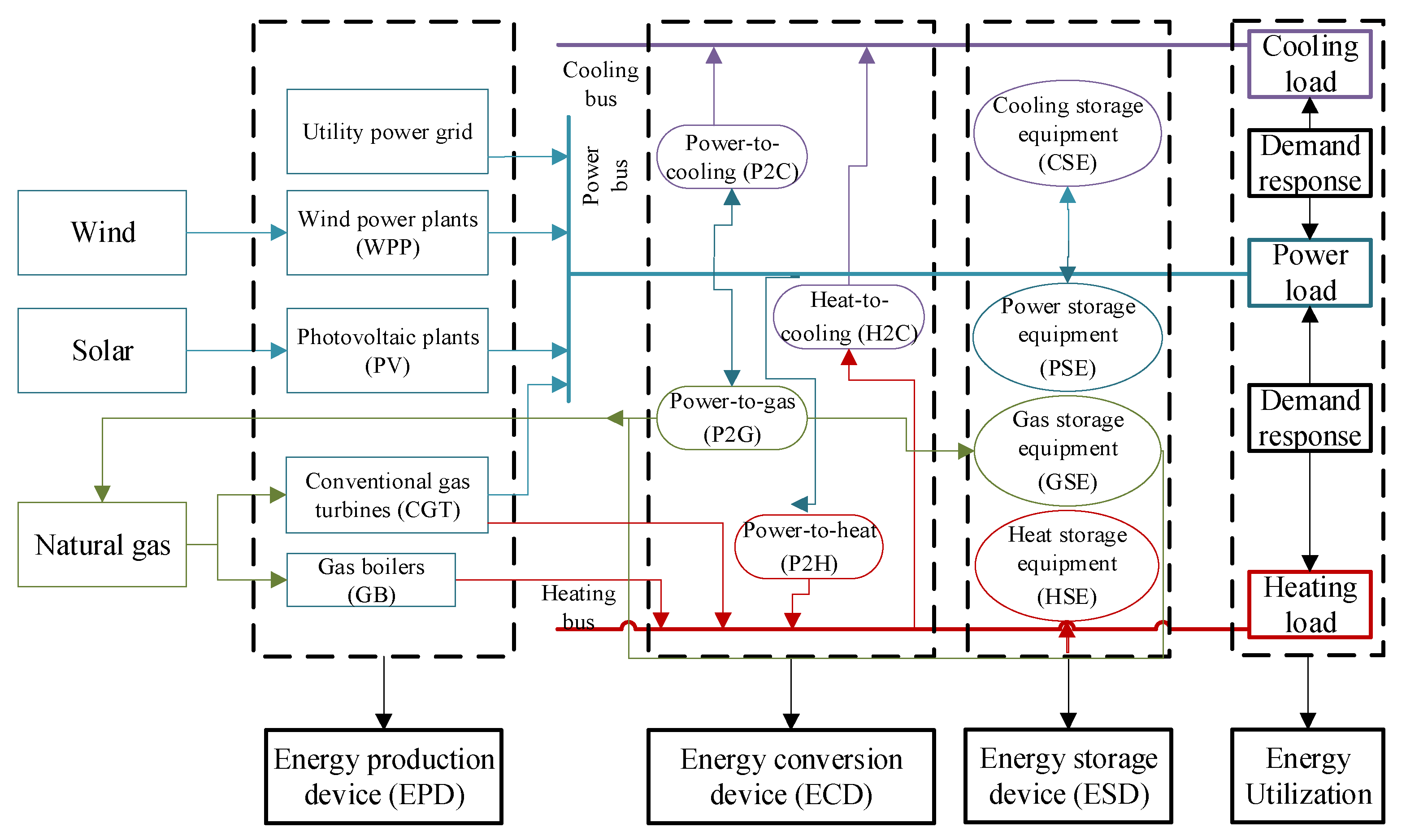
(1) The structure of the MES, with energy production, conversion, and storage devices, was designed. Also, an incentive-based demand–response (IBDR) and a price-based demand–response (PBDR) were introduced for optimizing the operation of the MES, and an operation model with uncertainty variables was constructed after uncertainties of the MES were analyzed.

(2) Three objectives, namely maximizing operating revenue, minimizing carbon emissions, and minimizing operational risk were pursued, and the constraints of supply–demand balance, unit operation, DR mechanism operation, and spinning reserve were considered.

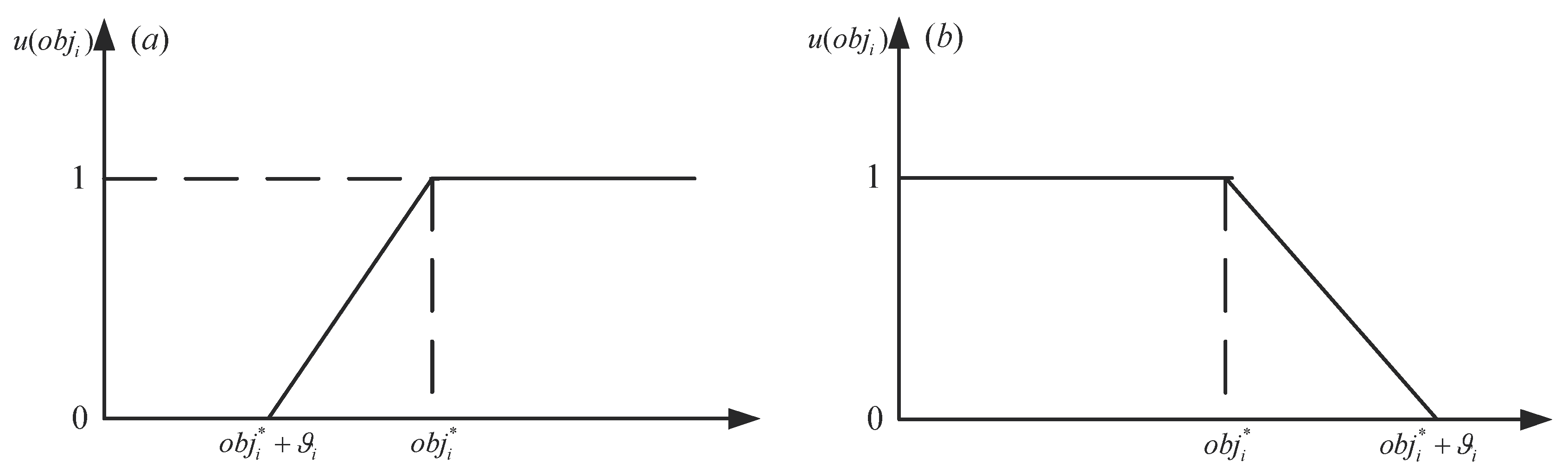
(3) A multi-objective solution algorithm for MES optimal operation based on fuzzy satisfaction theory and the rough set method was proposed. Firstly, the objective functions were processed using fuzzy satisfaction theory, and optimal dispatching strategies were established under single-objective functions. Then, a multi-objective input–output table was built and the functions’ weights were determined via the rough set method, thus obtaining a comprehensive dispatching optimization model. Finally, the effectiveness of the constructed model was verified by conducting a case study.

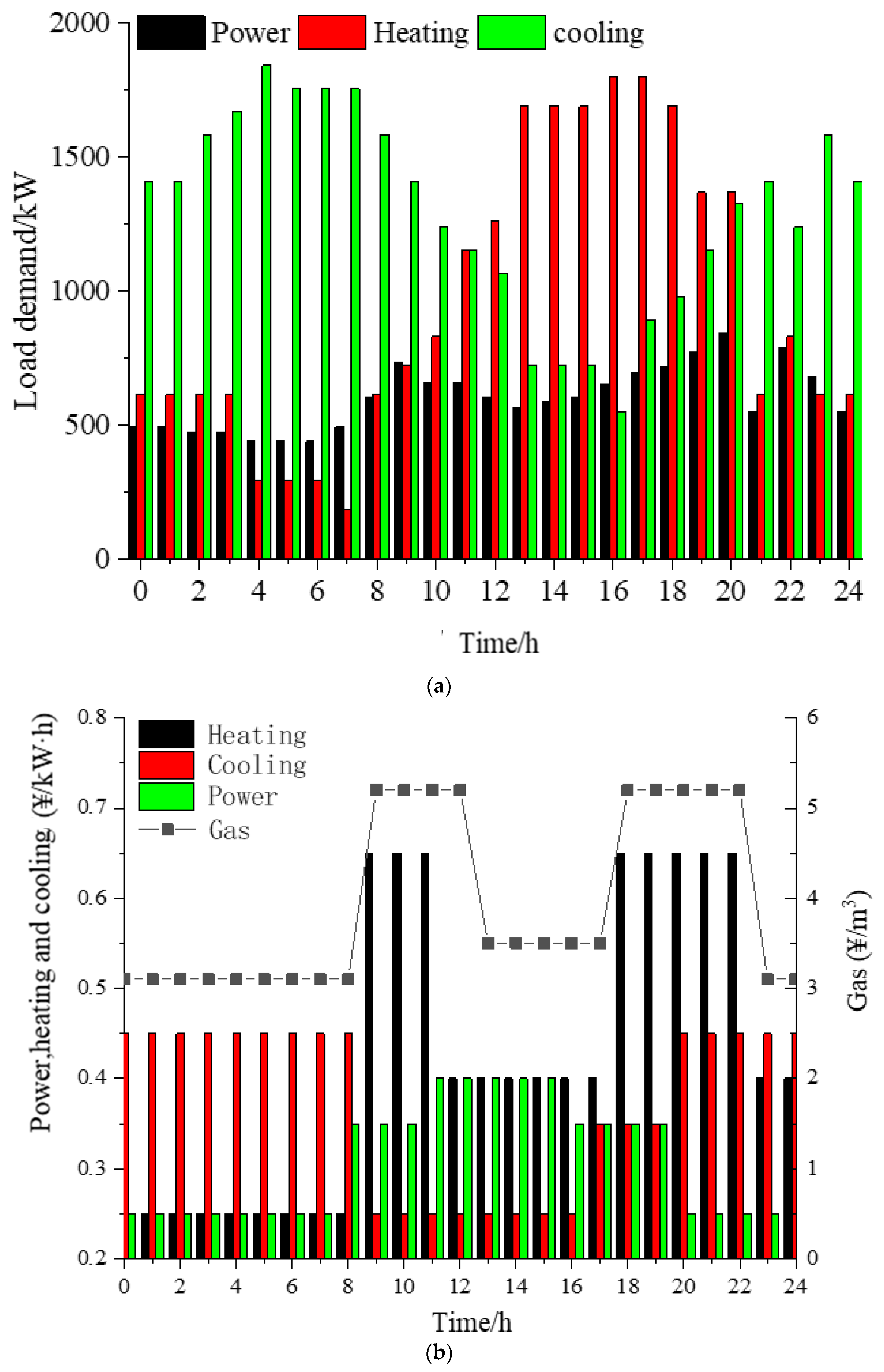
The remainder of this paper is laid out as follows. Section 2 introduces the core structure of the MES and constructs a probability distribution model with the uncertainties of the MES. Section 3 establishes a multi-objective coordinated dispatching optimization model for the MES, with the objectives of maximum operating revenue, minimum operational risk, and minimum carbon emissions. In Section 4, a multi-objective weighting method is established by combining the fuzzy satisfaction and rough set methods to solve the constructed model, thus obtaining a comprehensive dispatching optimization model. Next, data from Longgang commercial park in Shenzhen City are introduced for a case study to verify the effectiveness of the constructed model in Section 5. Significant findings are concluded in Section 6.

2. Description and Analysis of the MES

2.1. Structure Description

The MES in this paper contains energy production, conversion, and storage devices (EPD, ECD, and ESD, respectively). The EPD includes wind power plants (WPP), photovoltaic plants (PV), conventional gas turbines (CGT), and gas boilers (GB). The ECD consists of power-to-cooling (P2C), power-to-gas (P2G), power-to-heat (P2H), and heat-to-cooling (H2C). The ESD is composed of cooling storage equipment (CSE), heat storage equipment (HSE), gas storage equipment (GSE), and power storage equipment (PSE). In addition, energy utilization in the system is mainly power, cooling, and heat consumption. Figure 1 shows the structure of the MES.

According to Figure 1, the MES achieves the power–heat–cooling cascade supply via energy inter-conversion; in particular, gas from the P2G is used by the CGT for power and heat generation. Since there is flexible load, the PBDR and IBDR are introduced to guide users to engage in operational optimization of the MES. The former encourages users to use energy rationally via the time-of-use tariff, and the latter is to sign pre-protocols with users, which directly controls energy behaviors of users, thus realizing multi-energy coordinated supply of power, heat, and cooling.

2.2. Uncertainty Analysis

The uncertainties of the MES are from the WPP/PV outputs and load demands. One of the key parts of establishing an optimal MES strategy is to simulate these uncertainties.

2.2.1. Uncertainty Analysis of the wind power plants (WPP)

Uncertainty of the WPP is caused by natural wind, which is hard to predict. Some literature has verified that the Weibull distribution function is an excellent model for wind speed simulation [17]. The function is as follows.

$$f\left(v\right)=\frac{\phi }{\vartheta }{\left(\frac{v}{\vartheta }\right)}^{\phi -1}{e}^{-{\left(v/c\right)}^{\phi }}$$

(1)

where $v$ is the wind speed, and $\phi$ and $\vartheta$ are the shape and scale parameters, respectively, which can be calculated by the mean and variance of wind speed during this period based on statistics. After the simulation of wind speed via Equation (1), the WPP available output is given by:

$$g_{WPP,t}^{*}=\{\begin{array}{ll}0,& v_t\le v_{\mathrm{in}}\\ \frac{v-v_{\mathrm{in}}}{v_{\mathrm{R}}-v_{\mathrm{in}}}{g}_{\mathrm{R}},& v_{\mathrm{in}}\le v_t\le v_{\mathrm{R}}\\ g_{\mathrm{R}},& v_{\mathrm{R}}\le v_t\le v_{\mathrm{out}}\\ 0,& v_t\ge v_{\mathrm{out}}\end{array}$$

(2)

where $g_{\mathrm{R}}$ is the WPP rated output; $v_{\mathrm{in}}$, $v_{\mathrm{out}}$, and $v_{\mathrm{R}}$ are the cut-in, cut-out, and rated wind speeds, respectively; $v_t$ is the real-time wind speed over time t, and $g_{WPP,t}^{*}$ is the available output over time t.

2.2.2. Uncertainty Analysis of the photovoltaic plants (PV)

The uncertainty of the PV is caused by solar radiation intensity. Some literature has verified that the beta distribution function is an excellent model for solar radiation intensity stimulation [18]. The function is as follows.

$$f\left(\theta \right)=\{\begin{array}{ll}\frac{\Gamma \left(\omega \right)\Gamma \left(\psi \right)}{\Gamma \left(\omega \right)+\Gamma \left(\psi \right)}{\theta }^{\omega -1}{\left(1-\theta \right)}^{\psi -1},& 0\le \theta \le 1,\omega \ge 0,\psi \ge 0\\ 0,& otherwise\end{array}$$

(3)

where $\theta$ is the solar radiation, and $\omega$ and $\psi$ are the shape parameters of the beta distribution function, respectively, which can be calculated by the mean and variance of solar radiation intensity based on historical data [19]. Then, the PV available output is given by:

$$g_{PV,t}^{\ast }={\eta }_{PV}\times S_{PV}\times {\theta }_t$$

(4)

where $g_{PV,t}^{\ast }$ is the maximum PV output over time t, ${\eta }_{PV}$ and $S_{PV}$ are the radiation efficiency and area, respectively, and ${\theta }_t$ is the radiation intensity over time t.

2.2.3. Uncertainty Analysis of Load Demands

To simulate the uncertainty of load demands, it is divided into forecasting value and deviation, as follows.

$$L_t=L_t^{\mathrm{f}}+L_t^{\mathrm{e}}$$

(5)

where $L_t$ is the load demand over time t, and $L_t^{\mathrm{f}}$ and $L_t^{\mathrm{e}}$ are the forecasting results and errors, respectively. If the load forecasting errors obey the normal distribution $L_t^{\mathrm{e}}~[0,{\delta }_{L,t}^2]$ [4], then the load demands also obey the normal distribution $L_t^{}~[L_t^{\mathrm{f}},{\delta }_{L,t}^2]$.

Equations (1), (3), and (5) were used to determine the uncertainty distribution function of the MES. To analyze and control its uncertainties, existing papers have generated typical distribution scenarios to establish an optimal dispatching strategy. In fact, such a simulation method has a certain error, thus creating risks for the MES operation. Different from the existing research, this paper intends to use a conditional risk value to measure the MES uncertainty risk, and to construct a multi-objective coordinated dispatching model that considers revenue, risk, and carbon emissions.

3. Multi-Objective Dispatching Model

The WPP and PV in the MES have high economic and environmental benefits, yet their uncertainties also give rise to the risk of load loss. In addition, environmental protection consciousness means that carbon emissions are an important constraint in the MES operation. Carbon emissions are mainly from the CGT and GB, thus the WPP, PV, and utility power grid (UPG) will be utilized more often to satisfy load demands, which leads to a high operational risk and a high energy supply cost. Hence, the effects of the operating revenue, carbon emissions, and operational risk need to be considered comprehensively.

3.1. Objective Functions

3.1.1. Maximizing the Operating Revenue

The revenue of the MES is from the operation of the EPD, ECD, ESD, etc.

$$Max ob{j}_1={\displaystyle \sum _{t=1}^T\left[\underset{R_{\mathit{E}\mathit{P},t}}{\underbrace{\left(\begin{array}{l}{R}_{WPP,t}+R_{PV,t}+\\ R_{CGT,t}+R_{GB,t}\end{array}\right)}}+\underset{R_{\mathit{E}\mathit{C},t}}{\underbrace{\left(\begin{array}{l}{R}_{P2G,t}+R_{P2H,t}+\\ R_{P2C,t}+R_{H2C,t}\end{array}\right)}}+\underset{R_{\mathit{E}\mathit{S},t}}{\underbrace{\left(\begin{array}{l}{R}_{PS,t}+R_{GS,t}+\\ R_{HS,t}+R_{CS,t}\end{array}\right)}}+\underset{R_{other,t}}{\underbrace{\left(\begin{array}{l}{R}_{PBDR,t}+\\ R_{IBDR,t}\end{array}\right)}}\right]}$$

(6)

where $ob{j}_1$ is the objective function; $R_{WPP,t}$, $R_{PV,t}$, $R_{CGT,t}$, and $R_{GB,t}$ are the operating revenues of the WPP, PV, CGT, and GB over time t, respectively; $R_{P2G,t}$, $R_{P2H,t}$, $R_{P2C,t}$, and $R_{H2C,t}$ are the operating revenues of the P2G, P2H, P2C, and H2C over time t, respectively; $R_{PS,t}$, $R_{GS,t}$, $R_{HS,t}$, and $R_{CS,t}$ are the revenues from power, gas, heat, and cooling storage over time t, respectively; and $R_{PBDR,t}$ and $R_{IBDR,t}$ are the revenues from the PBDR and IBDR over time t, respectively. The operating revenue of the EPD is the energy supply income minus the energy supply cost. Since the WPP and PV have almost zero marginal cost, the energy supply cost is from the CGT.

$$\begin{array}{ll}{C}_{\mathrm{CGT},t}& =C_{\mathrm{CGT},t}^{\mathrm{fuel}}+C_{\mathrm{CGT},t}^{\mathrm{sd}}\\ & =\left\{\begin{array}{l}a{\left(g_{CGT,t}^{}+{\theta }_{\mathrm{h}}^{\mathrm{e}}{Q}_{CGT,t}^{}\right)}^2+\\ b\left(g_{CGT,t}^{}+{\theta }_{\mathrm{h}}^{\mathrm{e}}{Q}_{CGT,t}^{}\right)+c\end{array}\right\}+\left\{\begin{array}{l}\left[{\mu }_{CGT,t}^u(1-{\mu }_{CGT,t-1}^u)\right]C_{CGT,t}^u+\\ \left[{\mu }_{CGT,s}^d(1-{\mu }_{CGT,s+1}^d)\right]C_{CGT,s+1}^d\end{array}\right\}\end{array}$$

(7)

where $C_{\mathrm{CGT},t}^{\mathrm{fuel}}$ and $C_{\mathrm{CGT},t}^{\mathrm{sd}}$ are the fuel and start–stop costs of the CGT over time t, respectively; $g_{CGT,t}$ and $Q_{CGT,t}$ are the CGT power and heating outputs over time t, respectively; ${\theta }_{\mathrm{h}}^{\mathrm{e}}$ is the power–heat conversion coefficient of the CGT; $a$, $b$, and $c$ are the coefficients of energy supply cost of the CGT; ${\mu }_{CGT,t}^u$ represents the start-up status over time t; ${\mu }_{CGT,s}^d$ represents the shutdown status over time s; and $C_{CGT,t}^u$ and $C_{CGT,s+1}^d$ are the start-up cost over time t and the shutdown cost over time s + 1, respectively.

In terms of the ECD and ESD, the operating revenue is the energy supply income minus the energy consumption (or the energy storage) cost, as follows.

$$R_{\mathit{E}\mathit{C},t}=Q_{\mathit{E}\mathit{C},t}^{\mathrm{output}}{p}_{\mathit{E}\mathit{C}}^{\mathrm{output}}{\eta }_{\mathit{E}\mathit{C}}^{\mathrm{output}}-Q_{\mathit{E}\mathit{C},t}^{\mathrm{input}}{p}_{\mathit{E}\mathit{C}}^{\mathrm{input}}/{\eta }_{\mathit{E}\mathit{C}}^{\mathrm{input}}$$

(8)

$$R_{\mathit{E}\mathit{S},t}=Q_{\mathit{E}\mathit{S},t}^{\mathrm{dis}}{p}_{\mathit{E}\mathit{S}}^{\mathrm{dis}}{\eta }_{\mathit{E}\mathit{S}}^{\mathrm{dis}}-Q_{\mathit{E}\mathit{S},t}^{\mathrm{chr}}{p}_{\mathit{E}\mathit{S}}^{\mathrm{chr}}/{\eta }_{\mathit{E}\mathit{S}}^{\mathrm{chr}}$$

(9)

where $Q_{\mathit{E}\mathit{C},t}^{\mathrm{output}}$ and $Q_{\mathit{E}\mathit{C},t}^{\mathrm{input}}$ are the input and output of the ECD over time t, respectively; $p_{\mathit{E}\mathit{C}}^{\mathrm{output}}$ and $p_{\mathit{E}\mathit{C}}^{\mathrm{input}}$ are the energy consumption and supply prices of the ECD over time t, respectively; ${\eta }_{\mathit{E}\mathit{C}}^{\mathrm{output}}$ and ${\eta }_{\mathit{E}\mathit{C}}^{\mathrm{input}}$ are the energy consumption and supply efficiency, respectively; $Q_{\mathit{E}\mathit{S},t}^{\mathrm{dis}}$ and $Q_{\mathit{E}\mathit{S},t}^{\mathrm{chr}}$ are the energy release and storage of the ESD over time t, respectively; $p_{\mathit{E}\mathit{S}}^{\mathrm{dis}}$ and $p_{\mathit{E}\mathit{S}}^{\mathrm{chr}}$ are the energy release and storage prices of the ESD over time t, respectively; and ${\eta }_{\mathit{E}\mathit{S}}^{\mathrm{dis}}$ and ${\eta }_{\mathit{E}\mathit{S}}^{\mathrm{chr}}$ are the energy release and storage efficiency of the ESD, respectively.

The operating revenue of DR covers the revenues from the PBDR and IBDR. The former gains energy supply revenue while the latter reduces power shortage penalties.

$$R_{PBDR,t}={\displaystyle \sum _{t=1}^{24}\left[p_t^{\mathrm{before}}{L}_t^{\mathrm{before}}-p_t^{\mathrm{after}}{L}_t^{\mathrm{after}}\right]}$$

(10)

$$R_{IBDR,t}={\displaystyle \sum _{k\in \left\{\begin{array}{l}power,heating,\\ cooling,gas\end{array}\right\}}^{}\left\{\Delta L_t^{k,\mathrm{IB}}{p}_t^{k,\mathrm{IB}}-\Delta L_t^{k,\mathrm{shortage}}{p}_t^k\right\}}$$

(11)

where $p_t^{\mathrm{before}}$ and $p_t^{\mathrm{after}}$ are the energy prices before and after the implementation of the PBDR over time t, respectively; $L_t^{\mathrm{before}}$ and $L_t^{\mathrm{after}}$ are the energy demands before and after the implementation of the PBDR over time t, respectively; $\Delta L_t^{k,\mathrm{shortage}}$ is the shortage of energy k over time t; and $p_t^{k,\mathrm{IB}}$ and $p_t^k$ are the energy supply price of the IBDR and the real-time energy price over time t, respectively.

3.1.2. Minimizing the Carbon Emissions

The carbon emissions are mainly from the CGT, GB, and UPG (since some energy demands are satisfied by the UPG, its carbon emissions are considered as products of the MES). The objective function is as follows.

$$\min ob{j}_2={\displaystyle \sum _{t=1}^T\left\{\left[\begin{array}{l}{a}_{CGT}+b_{CGT}\left(g_{CGT,t}^{}+{\theta }_{\mathrm{h}}^{\mathrm{e}}{Q}_{CGT,t}^{}\right)+\\ c_{CGT}{\left(g_{CGT,t}^{}+{\theta }_{\mathrm{h}}^{\mathrm{e}}{Q}_{CGT,t}^{}\right)}^2\end{array}\right]+Q_{GB,t}{\psi }_{GB}^{{\mathrm{CO}}_2}+E_{UG,t}{\psi }_{UG}^{{\mathrm{CO}}_2}\right\}}$$

(12)

where $a_{CGT}$, $b_{CGT}$, and $c_{CGT}$ are the coefficients of carbon emissions of the CGT; $Q_{GB,t}$ is the heat supply of the GB over time t; ${\psi }_{GB}^{{\mathrm{CO}}_2}$ is the carbon emissions per unit from the GB; $E_{UG,t}$ is the energy supply of the UPG over time t, including power, heat, cooling, and gas; and ${\psi }_{UG}^{{\mathrm{CO}}_2}$ is the unit carbon emissions of the UPG. Currently, coal-fired power generation in China, for example, has accounted for 70% of overall power generation, and the coefficient of carbon emissions per unit power generation is approximately 0.997.

3.1.3. Minimizing the Operational Risk

The uncertainties of the WPP and PV bring greater risks to the MES. Measuring the risk level of MES operation is also one of the key parts of establishing an optimal scheduling strategy. This paper uses the “conditional value at risk” (CVaR) as a risk measuring factor for MES operation. Compared with the traditional “value at risk” (VaR) method, the CVaR can be used to describe the risk distribution outside the confidence level, which is conducive to overcoming the limitations that VaR only expresses risk situations at corresponding confidence levels without taking the risk tail into account. The introduction of the CVaR is detailed in [19]. The objective function based on the CVaR is as follows.

$$\min ob{j}_3=\alpha +\frac{1}{1-\beta }{\displaystyle \underset{\mathit{e}\in {\mathit{R}}^m}{\int }{\left(f\left(E,e\right)-\alpha \right)}^{+}p\left(e\right)de}$$

(13)

Equation (13) is used to calculate the CVaR of the MES, in which $\alpha$ is the MES operation loss’ critical value, which is for determination of MES operational risk situations; $f\left(E,e\right)$ is the loss function of MES operation, which equals $-ob{j}_1$; $E^T=\left[E_{MEG,t}\left(1\right),g_{MEG,t}\left(2\right),\cdots ,g_{MEG,t}\left(T\right)\right]$ is a decision vector; $e^T=\left[g_{WPP,t},g_{PV,t},L_t\right]$ is a multivariate random vector; and $\beta$ is the confidence of MES operation. The minimum $\alpha$, namely, the VaR, is calculated by Equation (13). The expected value is replaced with N samples of random vector $e$, namely, $e_1,e_2,\cdots ,e_{\mathrm{N}}$, because it is hard to obtain directly.

$$\min ob{j}_3=\alpha +\frac{1}{N\left(1-\beta \right)}{\displaystyle \sum _{k=1}^N{\left(f\left(E,e\right)-\alpha \right)}_k^{+}}$$

(14)

Above all, the uncertainties of the objective functions have been described by the CVaR method, and the risk-avoiding optimization model has been built, which is an effective tool for different decision makers to make dispatching strategies for different interests.

3.2. Constraints

Supply–demand balance, operation constraints of the EPD, ECD, and ESD, and system spinning reserve need to be satisfied in the process of the MES operational optimization.

3.2.1. Supply–Demand Balance

$$g_{CGT,t}^{}+g_{WPP,t}+g_{PV,t}+g_{\mathrm{P}2\mathrm{G},t}^{\mathrm{output}}+g_{PS,t}^{\mathrm{dis}}=L_t^{\mathrm{e}}+g_{PS,t}^{\mathrm{chr}}+g_{\mathrm{P}2\mathrm{G},t}^{\mathrm{input}}+g_{\mathrm{P}2\mathrm{H},t}^{\mathrm{input}}+g_{\mathrm{P}2\mathrm{C},t}^{\mathrm{c},\mathrm{input}}+\Delta L_t^{\mathrm{p},\mathrm{PB}}+\Delta L_t^{\mathrm{p},IB}$$

(15)

$$Q_{CGT,t}^{}+Q_{GB,t}^{}+Q_{\mathrm{P}2\mathrm{H},t}^{\mathrm{output}}+Q_{\mathrm{HS},t}^{\mathrm{dis}}=L_t^{\mathrm{h}}+Q_{\mathrm{HS},t}^{\mathrm{chr}}+Q_{\mathrm{H}2\mathrm{C},t}^{\mathrm{input}}+\Delta L_t^{\mathrm{h},\mathrm{PB}}+\Delta L_t^{\mathrm{h},\mathrm{IB}}$$

(16)

$$Q_{\mathrm{P}2\mathrm{C},t}^{\mathrm{output}}+Q_{\mathrm{H}2\mathrm{C},t}^{\mathrm{output}}+Q_{\mathrm{CS},t}^{\mathrm{dis}}=L_t^{\mathrm{c}}+Q_{\mathrm{CS},t}^{\mathrm{chr}}+\Delta L_t^{\mathrm{c},\mathrm{PB}}+\Delta L_t^{\mathrm{c},\mathrm{IB}}$$

(17)

where $Q_{GB,t}^{}$ is the GB heating output over time te; $g_{\mathrm{P}2\mathrm{G},t}^{\mathrm{input}}$ and $g_{\mathrm{P}2\mathrm{G},t}^{\mathrm{output}}$ are the power consumption and gas generation of the P2G over time te, respectively; $g_{\mathrm{P}2\mathrm{H},t}^{\mathrm{input}}$ and $g_{\mathrm{P}2\mathrm{C},t}^{\mathrm{c},\mathrm{input}}$ are the P2H and P2C power consumptions over time te, respectively; $Q_{\mathrm{P}2\mathrm{H},t}^{\mathrm{output}}$ is the P2H heating output over time t; $Q_{\mathrm{HS},t}^{\mathrm{input}}$ and $Q_{\mathrm{HS},t}^{\mathrm{output}}$ are the HSE heat storage and release over time t, respectively; $Q_{\mathrm{H}2\mathrm{C},t}^{\mathrm{input}}$ is the H2C heat consumption over time t; $\Delta L_t^{\mathrm{h},\mathrm{PB}}$ is the PBDR heating output over time t; $Q_{\mathrm{P}2\mathrm{C},t}^{\mathrm{output}}$ and $Q_{\mathrm{H}2\mathrm{C},t}^{\mathrm{output}}$ are the cooling outputs of the P2C and H2C over time t, respectively; $Q_{\mathrm{CS},t}^{\mathrm{input}}$ and $Q_{\mathrm{CS},t}^{\mathrm{output}}$ are the cooling storage and release of the CSE over time t, respectively; $\Delta L_t^{\mathrm{p},IB}$ is the IBDR power output over time t, $\Delta L_t^{\mathrm{h},\mathrm{IB}}$ is the IBDR heating output over time t; and $\Delta L_t^{\mathrm{c},\mathrm{PB}}$ is the PBDR cooling output over time t. The PBDR is given by the price elasticity of demand [20].

$$E_{st}=\frac{\Delta Q_s/Q_s^0}{\Delta P_t/P_t^0}\{\begin{array}{l}{E}_{st}\le 0,s=t\\ E_{st}\ge 0,s\ne t\end{array}$$

(18)

where $\Delta Q_s$ and $\Delta P_t$ are the changes in demand and price following the implementation of PBDR. The variations of power, heating, and cooling load following the implementation of the PBDR are given by:

$$\Delta L_t^{\left(\mathrm{p},\mathrm{h},\mathrm{c}\right),\mathrm{PB}}=Q_t^{e,h,c}\times \left\{E_{tt}^{\mathrm{p},\mathrm{h},\mathrm{c}}\times \frac{\left[P_t^{\mathrm{p},\mathrm{h},\mathrm{c}}-P_t^{\left(\mathrm{p},\mathrm{h},\mathrm{c}\right),0}\right]}{P_t^{\left(\mathrm{p},\mathrm{h},\mathrm{c}\right),0}}+{\displaystyle \sum _{\begin{array}{l}s=1\\ s\ne t\end{array}}^{24}{E}_{st}^{\mathrm{p},\mathrm{h},\mathrm{c}}}\times \frac{\left[P_s^{\mathrm{p},\mathrm{h},\mathrm{c}}-P_s^{\left(\mathrm{p},\mathrm{h},\mathrm{c}\right),0}\right]}{P_s^{\left(\mathrm{p},\mathrm{h},\mathrm{c}\right),0}}\right\}$$

(19)

where $\Delta L_t^{\left(\mathrm{p},\mathrm{h},\mathrm{c}\right),\mathrm{PB}}$ and $Q_t^{e,h,c}$ are the load variations and initial load, respectively; $P_t^{\mathrm{p},\mathrm{h},\mathrm{c}}$ and $P_t^{\left(\mathrm{p},\mathrm{h},\mathrm{c}\right),0}$ are power, heating, and cooling prices before and after the implementation of the PBDR over time t, respectively; and $E_{tt}^{\mathrm{p},\mathrm{h},\mathrm{c}}$ represents the price elasticities of power, heating, and cooling demands. When $s=t$, $E_{tt}^{\mathrm{p},\mathrm{h},\mathrm{c}}$ is called self-elasticity, otherwise it is known as cross-elasticity. The description is detailed in [20].

3.2.2. Operation Constraints of the demand response (DR)

$$\Delta L_t=\left(u_t^{\mathrm{IB}}\Delta L_t^{\mathrm{IB}}+u_t^{\mathrm{PB}}\Delta L_t^{\mathrm{PB}}\right)$$

(20)

$$u_t\Delta L_{}^{-}\le \Delta L_t-\Delta L_{t-1}\le u_t\Delta L^{+}$$

(21)

$$(T_{t-1}^{\mathrm{on}}-M_{}^{\mathrm{on}})(u_{t-1}-u_t)\ge 0$$

(22)

$$(T_{t-1}^{\mathrm{off}}-M_{}^{\mathrm{off}})(u_t-u_{t-1})\ge 0$$

(23)

where $\Delta L_t$ is the energy supply of the DR over time t, including the PBDR and IBDR; $\Delta L_{}^{-}$ and $\Delta L^{+}$ are the ramping power restrictions; $T_{t-1}^{\mathrm{on}}$ is the operational duration of the DR over time t − 1; $M_{}^{\mathrm{on}}$ is the minimum start-up time of the DR; $T_{t-1}^{\mathrm{off}}$ is the duration when the DR has been off before time t; and $M_{}^{\mathrm{off}}$ is the minimum time it takes to stop the DR.

3.2.3. Operation Constraints of the Energy Production Device (EPD)

The EPD includes the WPP, PV, CGT, and GB, all of which need to satisfy the maximum output constraints, which are detailed in [20]. In terms of CGT, the relationship between power output and heating output is called “electrothermal characteristics”. Under the given heating output, the power generation has adjustability. This is because CGT adjusts its power output by adjusting the steam generation of condensate under the given extraction capacity. The larger the extraction capacity, the smaller the proportion of adjustable condensate generating steam, and the smaller the adjustment range. The constraints are as follows.

$$\max \left\{g_{CGT}^{\min }-c_{\min }{Q}_{CGT}^{},c_m\left(Q_{CGT}^{}-Q_{CGT}^{{}_0}\right)\right\}\le g_{CGT}^{}\le g_{CGT}^{\max }-c_{\max }{Q}_{CGT}^{}$$

(24)

$$u_{CGT,t}\Delta g_{CGT}^{-}\le \left(g_{CGT,t}^{}+{\theta }_{\mathrm{h}}^{\mathrm{e}}{Q}_{CGT,t}^{}\right)-\left(g_{CGT,t-1}^{}+{\theta }_{\mathrm{h}}^{\mathrm{e}}{Q}_{CGT,t-1}^{}\right)\le u_{CGT,t}\Delta g_{CGT}^{+}$$

(25)

where $c_{\min }$ and $c_{\max }$ are the $c$ values under the minimum and maximum power output, respectively; $c$ is the reduction of power generation under the condition of extracting more units of heat when the intake of steam is constant; $c_m=\Delta g_{CGT}^{}/\Delta Q_{CGT}^{}$ is the power/heating elasticity coefficient during back pressure operation; $Q_{CGT}^{{}_0}$ is a constant; $Q_{CGT}^{\max }$ is the maximum CGT heating output; $Q_{CGT}^{\min }$ is the heating output while the CGT generates minimum electric power; $g_{CGT}^{\min }$ and $g_{CGT}^{\max }$ are the minimum and maximum CGT power outputs under the condition of pure condensation, respectively; $\Delta g_{CGT}^{-}$ and $\Delta g_{CGT}^{+}$ are the ramping restrictions; and $u_{CGT}$ is the CGT operation status. The CGT and GB also need to satisfy the ramping constraints, as well as start-up and shutdown time constraints, which are similar to Equations (20)–(23).

3.2.4. Operation Constraints of the energy conversion device (ECD)

The ECD contains the P2H, P2C, H2C, and P2G. Equation (8) is used to determine the energy conversion relationships among different devices. Although the conversion efficiency is variable, it does not change significantly when the devices operate stably. According to [20], the efficiency is considered as a constant, and the mathematical model is as follows.

$$\left[\begin{array}{c}{V}_{\mathrm{P}2\mathrm{G},t}\\ Q_{\mathrm{P}2\mathrm{C},t}\\ Q_{\mathrm{P}2\mathrm{H},t}\\ Q_{\mathrm{H}2\mathrm{C},t}\end{array}\right]=\left[\begin{array}{cccc}{g}_{\mathrm{P}2\mathrm{G},}{}_t& 0& 0& 0\\ 0& g_{\mathrm{P}2\mathrm{C},t}& 0& 0\\ 0& 0& g_{\mathrm{P}2\mathrm{H},}{}_t& 0\\ 0& 0& 0& Q_{\mathrm{H}2\mathrm{C},}{}_t\end{array}\right]\left[\begin{array}{c}{\eta }_{\mathrm{P}2\mathrm{G}}\\ {\eta }_{\mathrm{P}2\mathrm{C}}\\ {\eta }_{\mathrm{P}2\mathrm{H}}\\ {\eta }_{\mathrm{H}2\mathrm{C}}\end{array}\right]$$

(26)

where $Q_{\mathrm{P}2\mathrm{C},t}$ is the P2C cooling output over time t; $Q_{\mathrm{P}2\mathrm{H},t}$ is the P2H heating output over time t; $Q_{\mathrm{H}2\mathrm{C},t}$ is the H2C cooling output over time t; $g_{\mathrm{P}2\mathrm{C},t}$ and $g_{\mathrm{P}2\mathrm{H},}{}_t$ are the power consumptions of the P2C and P2H over time t, respectively; $Q_{\mathrm{H}2\mathrm{C},}{}_t$ is the H2C heat consumption over time t; and ${\phi }_{\mathrm{P}2\mathrm{C}}$, ${\phi }_{\mathrm{P}2\mathrm{H}}$, and ${\phi }_{\mathrm{H}2\mathrm{C}}$ are the energy conversion efficiencies of the P2C, P2H, and H2C, respectively.

$$u_{EC,t}^{\mathrm{output}}{E}_{EC,t}^{\mathrm{output},\min }\le E_{EC,t}^{\mathrm{output}}\le u_{EC,t}^{\mathrm{output}}{E}_{EC,t}^{\mathrm{output},\max }$$

(27)

$$u_{EC,t}^{\mathrm{input}}{E}_{EC,t}^{\mathrm{input},\min }\le E_{EC,t}^{\mathrm{input}}\le u_{EC,t}^{\mathrm{input}}{E}_{EC,t}^{\mathrm{input},\max }$$

(28)

where $E_{EC,t}^{\mathrm{output},\min }$ and $E_{EC,t}^{\mathrm{output},\max }$ are the ECD energy supply boundaries over time t, respectively; $E_{EC,t}^{\mathrm{input},\min }$ and $E_{EC,t}^{\mathrm{input},\max }$ are the ECD energy consumption boundaries over time t, respectively; and $u_{EC,t}^{\mathrm{output}}$ and $u_{EC,t}^{\mathrm{input}}$ are the ECD status variables over time t, respectively.

3.2.5. Operation Constraints of the energy storage device (ESD)

The ESD contains the PSE, HSE, CSE, and GSE. Different types of ESD can store and release energy according to supply–demand relationships. The operation model is as follows.

$$S_{ES,t}=\left(1-{\eta }_{ES,t}^{\mathrm{loss}}\right)S_{ES,t-1}+\left[E{S}_t^{\mathrm{input}}{\eta }_{ES}^{\mathrm{input}}-E{S}_t^{\mathrm{output}}/{\eta }_{ES}^{\mathrm{output}}\right]$$

(29)

$$S_{ES,t}^{\min }\le S_{ES,t}^{}\le S_{ES,t}^{\max }$$

(30)

$$S_{ES,T_0}^{}=S_{ES,T}^{}$$

(31)

where $S_{ES,t}$ is the ESD energy storage over time t; ${\eta }_t^{\mathrm{loss}}$ is the ESD energy loss rate over time t; $E{S}_t^{\mathrm{input}}$ and $E{S}_t^{\mathrm{output}}$ are the energy storage and release of the ESD over time t, respectively; ${\eta }_{ES}^{\mathrm{input}}$ and ${\eta }_{ES}^{\mathrm{output}}$ are the ESD energy storage and release efficiencies over time t, respectively; and $S_{ES,t}^{\min }$ and $S_{ES,t}^{\max }$ are the ESD energy storage boundaries over time t, respectively. To reserve some adjustment margin, the devices are restored to the initial storage energy after one cycle of operation. $T_0$ and $T$ are the beginning and end of adjustment cycle, respectively.

3.2.6. Constraints of Carbon Emissions

The maximum total emission allowance (MTEA) is introduced to limit carbon emissions.

$$ob{j}_2\le META$$

(32)

where $META$ is the maximum allowable carbon emissions.

3.2.7. Spinning Reserve Constraints

The MES is set to run in “following thermal load” mode, so it is necessary to reserve some power capacity and cooling capacity. Moreover, reserve capacity is required due to the WPP/PV uncertainties. The constraints are as follows.

$$g_{MEG,t}^{\mathrm{p},\max }-g_{MEG,t}^{\mathrm{p}}+g_{PS,t}^{\mathrm{dis}}+\Delta L_t^{\mathrm{p},IB}+{\left[L_t^{\mathrm{p},\mathrm{after}}-L_t^{\mathrm{p},\mathrm{before}},0\right]}^{+}\ge r_{\mathrm{p}}{L}_t^{\mathrm{p}}+r_{WPP}^{\mathrm{up}}{g}_{WPP,t}+r_{PV}^{\mathrm{up}}{g}_{PV,t}$$

(33)

$$g_{MEG,t}^{\mathrm{p}}-g_{MEG,t}^{\mathrm{p},\min }+g_{PS,t}^{\mathrm{chr}}+{\left[L_t^{\mathrm{p},\mathrm{after}}-L_t^{\mathrm{p},\mathrm{before}},0\right]}^{-}\ge r_{WPP}^{\mathrm{dn}}{g}_{WPP,t}+r_{PV}^{\mathrm{dn}}{g}_{PV,t}$$

(34)

$$g_{MEG,t}^{\mathrm{c},\max }-g_{MEG,t}^{\mathrm{c}}+g_{CS,t}^{\mathrm{dis}}+{\left[L_t^{\mathrm{c},\mathrm{after}}-L_t^{\mathrm{c},\mathrm{before}},0\right]}^{+}\ge r_{\mathrm{c}}{L}_t^{\mathrm{c}}$$

(35)

where $g_{MEG,t}$ is the MES power output over time t; $g_{MEG,t}^{\mathrm{p},\max }$ and $g_{MEG,t}^{\mathrm{p},\min }$ are the MES power output boundaries over time t, respectively; $r_{\mathrm{e}}$ and $r_{\mathrm{c}}$ are the upper spinning reserve coefficients of the power and cooling loads, respectively; $r_{WPP}^{\mathrm{up}}$/$r_{PV}^{\mathrm{up}}$ and $r_{WPP}^{\mathrm{dn}}$/$r_{PV}^{\mathrm{dn}}$ are the WPP and PV’s upper and lower spinning reserve coefficients, respectively.

4. Solution Algorithms

4.1. Fuzzy Linearization

4.1.1. Objective Function Fuzzification

In multi-objective optimization, the objective functions are jointly transformed into a comprehensive single-objective optimization model, usually by weighting them. The objective functions of this paper include the maximum operating revenue, minimum operational risk, and minimum carbon emissions. Different dimensions and optimizing directions of the objectives make it difficult to directly weight them, thus preprocessing is performed. Fuzzy satisfaction theory is used to transform the numerical optimization into the degree optimization by analyzing the distance between the objective function value and the ideal value [21]. A semi-linear membership function and semi-gradient membership function are introduced in this paper, and the former is used to maximize the operating revenue, while the latter is used to minimize the operational risk and carbon emissions. The process is as follows.

$$\rho (ob{j}_i)=\{\begin{array}{l}0, ob{j}_i\le ob{j}_i^{*}\\ \frac{ob{j}_i^{*}+{\vartheta }_i-ob{j}_i}{{\vartheta }_i}, ob{j}_i^{*}<ob{j}_i^{}<ob{j}_i^{*}+{\vartheta }_i\\ 1, ob{j}_i>ob{j}_i^{*}+{\vartheta }_i\end{array}$$

(36)

Equation (36) is the semi-linear membership function, and $\rho (ob{j}_i)$ is the membership function of $ob{j}_i$. In addition, $ob{j}_i$, $ob{j}_i^{*}$, and ${\vartheta }_i$ are the actual value, ideal value, and acceptable added value of the i-th objective function, respectively (${\vartheta }_i$ therein is used to scale the objective).

$$\rho (ob{j}_i)=\{\begin{array}{l}1, ob{j}_i\ge ob{j}_i^{*}\\ \frac{ob{j}_i-\left(ob{j}_i^{*}+{\vartheta }_i\right)}{{\vartheta }_i}, ob{j}_i^{*}<ob{j}_i<ob{j}_i^{*}+\vartheta \\ 0, ob{j}_i\le ob{j}_i^{*}\end{array}$$

(37)

Equation (37) is the semi-gradient membership function. Figure 2 shows the semi-linear membership and the semi-gradient membership functions.

4.1.2. Linearization of Mathematical Models

Equations (6), (12), and (14) are used to determine the multi-objective dispatching optimization model for the MES. There are quadratic terms in the objective functions and the operation constraints, which makes the constructed model a mixed integer nonlinear programming problem (MINLP). The MINLP is hard to directly solve and its solutions may not be optimum, so the constraints and objectives were linearized before solving the model. Taking Equation (7) for example, this means ${g^{\prime }}_{CGT,t}^{}$ is set equal to $g_{CHP,t}^e+{\theta }_h^e{Q}_{CHP,t}^h$, belonging to $\left[g_{CHP}^{\min },g_{CHP}^{\mathrm{m}ax}\right]$, and ${g^{\prime }}_{CGT,t}^{}$ is divided into N segments. Then, the length of each segment is $\Delta g_{CGT}$, so $C\left(g_{CGT}\right)$ can be expressed as a piecewise function when $g_{CGT,t}^{}\in \left[g_{CGT,t}^{\min }+n\Delta g_{CGT},g_{CGT,t}^{\max }+\left(n+1\right)\Delta g_{CGT}\right]$.

$$C\left(g_{CGT,t}\right)=f^{\prime }\left(g_{CGT}^{\min }+n\Delta g_{CGT}^{}\right)+\left(g_{CGT,t}-g_{CGT}^{\min }-n\Delta g_{CGT}^{}\right)\times \left[b_{CGT}+(2n+1)c_{CGT}\cdot \Delta g_{CGT}^{}+2c_{CGT}{g}_{CGT}^{\min }\right]$$

(38)

where $n=0,1,\dots ,N-1$ and $\Delta g_{CGT}^{}=(g_{CGT}^{\max }-g_{CGT}^{\min })/N$. Similarly, the outputs of other quadratic terms are the same as for Equation (15). The maximum relative error does not exceed 1%, and most often it is below 0.5%, when $N\ge 5$. Figure 3 shows the linearization process.

Similarly, Equations (21)–(23) can be linearized, and the process is as follows.

$${\displaystyle \sum _{\tau =t}^{T_1}{u}_{CGT,t}\ge T_{CGT,t}^{on}{M}_{CGT}^{on}}, T_1=t+M_{CGT}^{on}-1, \forall t=L+1,\dots \dots ,T-M_{CGT}^{on}+1$$

(39)

$${\displaystyle \sum _{\tau =t}^{T_2}\left[1-u_{CGT,t}\right]\ge T_{CGT,t}^{off}{M}_{CGT}^{off},} T_2=t+M_{CGT}^{off}-1, \forall t=D+1,\dots \dots ,T-M_{CGT}^{off}+1$$

(40)

$${\displaystyle \sum _{\tau =t}^T\left[u_{CGT,t}-T_{CGT}^{on}\right]}\ge 0 \forall t=T-M_{CGT}^{off}+2,\dots \dots ,T$$

(41)

$${\displaystyle \sum _{\tau =t}^T\left[1-u_{CGT,t}-T_{CGT,t}^{off}\right]}\ge 0 \forall t=T-M_i^{off}+2,\dots \dots ,T$$

(42)

where $L$ is the number of the CGTs in the initial state. L = 0 if it is not in the initial state. D is the number of the CGTs which are not in the initial state. After that, the MINLP has been changed into a mixed integer programming model.

4.2. Rough Set Weighting Method

The objective functions’ optimal weights need to be determined next. In general, the weighting method includes subjective weighting and objective weighting methods. The former is mainly based on subjective experience, which can make the best of decision makers’ empirical knowledge, but it is subject to the subjective influence of decision makers; thus, the weights may have errors. The latter relies on objective data, and the weights can be determined using mathematical theories and methods, which overcomes the shortcomings of subjective weighting methods. To calculate weights, this paper proposes a concept of a payoff table. Not only are obj_i (i = 1, 2, …, I) taken as optimizing objectives to solve the constructed model, but also other objective values are obtained under this objective. The multi-objective function payoff table is shown below.

Based on

Table 1. Payoff table of multi-objective functions.

Objective Function	Function Value
	$\mathit{o}\mathit{b}{\mathit{j}}_1$	$\mathit{o}\mathit{b}{\mathit{j}}_2$	…	$\mathit{o}\mathit{b}{\mathit{j}}_{\mathbf{I}}$
obj1	obj11	obj12	…
obj2	obj21	$\ddots$
⋮	⋮	⋮	$\ddots$
objI	objI1	objI2	…	objII

, the preprocessed decision matrix [obj_ik]I × I is determined. The rough set weighting method is used to gain the optimal weights. This method processes incomplete and inaccurate data through learning, induction, and mining, and finally a clear and concise data system is established [22]. Figure 4 shows the weighting process of multi-objective functions.

4.2.1. Constructing the Relational Data Model

The weight of function $f_i$ is set to $1/\mathrm{I}$, and $\tilde{F}$ of the comprehensive objective is calculated. Here, $\tilde{F}$ is the decision attribute and $D=\left\{\tilde{F}\right\}$ is the decision attribute set. $U=\left\{u_1,u_2,\dots ,u_j\right\}$ is the sample set, $u_j=(f_{1j},f_{2j},\dots ,f_{mj};{\tilde{F}}_j)$, and $u_k$ is the comprehensive objective’s optimal value, which represents information on object F. The attribute of $u_k$ is $f_i(u_j)=v_{ij}$, and $F_i(u_j)={\tilde{F}}_j$.

4.2.2. Calculating the Dependence of $R_V$ on $R_{\mathrm{D}}$

$$r_{R_V}(R_{\mathrm{D}})=\frac{{\displaystyle \sum \rho [R_V({[\tilde{F}]}_{R_{\mathrm{D}}})]}}{\rho (U)}$$

(43)

where $R_V$ and $R_{\mathrm{D}}$ are knowledge bases, $r_{R_V}(R_{\mathrm{D}})$ is the dependence of $R_V$ on $R_{\mathrm{D}}$, $\rho (·)$ is the set base, and $p_v(D)$ represents all the knowledge classified by using U/C in U, which is used to determine the equivalent classification of the objective set in U/D.

4.2.3. Calculating the Dependence of $R_V$ on $R_{V-\left|v_i\right|}$

$$r_{R_{V-\left|v_i\right|}}(R_{\mathrm{D}})=\frac{{\displaystyle \sum \rho [R_{V-\left|v_i\right|}({[\tilde{F}]}_{R_{\mathrm{D}}})]}}{\rho (U)}$$

(44)

where $r_{R_{V-\left|v_i\right|}}(R_{\mathrm{D}})$ is the dependence of $R_V$ on $R_{V-\left|v_i\right|}$, and $p_{V-\left|v_i\right|}(D)$ represents all the knowledge classified by using U/C in $U$ after index $V_i$ is dropped.

4.2.4. Calculating the Weight of Object i

$${\sigma }_{\mathrm{D}}(D)=r_{R_V}(D)-r_{R_{V-\left|v_i\right|}}(D)$$

(45)

$${\lambda }_i={\sigma }_{\mathrm{D}}(v_i)/{\displaystyle \sum _{i=1}^I{\sigma }_{\mathrm{D}}(v_i)}$$

(46)

where ${\sigma }_{\mathrm{D}}(D)$ is the importance degree of object i, and ${\lambda }_i$ is the weight of each objective function. The comprehensive single-objective function is given by:

$$\begin{array}{l}OBJ={\displaystyle \sum _{i=1}^I{\lambda }_i\mu (ob{j}_i)}\\ s.t.\{\begin{array}{l}\mathrm{Equation} \left(15\right)-\mathrm{Equation} \left(20\right)\\ \mathrm{Equation} (24)-\mathrm{Equation} (35)\\ \mathrm{Equation} (39)-\mathrm{Equation} (42)\\ z_k=f\left(E,e\right)-\alpha \\ z_k\ge 0\\ \mathrm{other} \mathrm{constriants}\end{array}\end{array}$$

(47)

where $OBJ$ is the comprehensive function, and its solution is the most satisfactory solution of the MES dispatch when considering all objective functions.

5. Case Study

5.1. Basic Data

To verify the effectiveness of the constructed model and solution algorithm, data from Longgang commercial park in Shenzhen City were selected for a case study [17]. This park employs WPP 1600 kW, PV 1000 kW, CGT 3200 kW, and GB 500 kW. The CGT includes a TAURUS60 CGT (CATERPILLAR, Beijing, China) with rated power of 2000 kW and a CENTAUR40 CGT (CATERPILLAR, Beijing, China) with rated power of 1200 kW. The CGT power generation cost is linearized into two parts, according to [22], which are 0.239 ¥/kW and 0.273 ¥/kW (TAURUS60 CGT), and 0.137 ¥/kW and 0.342 ¥/kW (CENTAUR40 CGT). The P2H with a capacity of 1500 kW, the P2C with 2000 kW, the H2C with 1500 kW, and the P2G with 200 kW were employed to achieve cascade utilization of multiple energy resources. Based on [22], power, heating, and cooling demands on a typical day, as well as the WPP and PV available outputs, were determined. The maximum demands of power, heating, and cooling were 2400 kW, 3640 kW, and 3696 kW, respectively. Figure 5 shows the demands and prices of power, heating, and cooling, as well as the available outputs of the WPP and PV, on a typical day.

This paper considers that the EPD, ECD, and ESD belong to the same owner. The energy prices in the MES are executed according to the prices at different times during a typical day (see Figure 5). According to [22], the parameters of the WPP are set to $v_{in}=3 \mathrm{m}/s$, $v_{rated}=14 \mathrm{m}/s$, and $v_{out}=25 \mathrm{m}/s$; the parameters $\alpha$ and $\beta$ of the PV are 0.39 and 8.54. Sampling WPP and PV power generation scenarios, 10 typical scenarios are generated, and the scenario with maximum occurrence probability is selected as the actual value. The on-grid power prices of the WPP and PV are set to be 0.54 ¥/kW·h and 0.83 ¥/kW·h, and the power supply price and heating price of the CGT are 0.35 ¥/kW·h and 0.25 ¥/kW·h. To promote WPP/PV on-grid connection, the power consumption price for energy conversion is set to be 0.25 ¥/kW·h, and the heat consumption price is 0.2 ¥/kW·h. Figure 6 shows the WPP and PV available outputs on a typical day.

Energy is stored during valley periods and released during peak periods to make the net load demand curve smoother. The PSE, HSE, and CSE capacities are all 1500 kW·h with the maximum storage/release power of 300 kW, and the capacity of the GSE is 800 m³ with the maximum storage/release of 150 m³. To study the DR’s optimizing effect on the MES, a day is divided into peak, valley, and flat periods for power, heating, and cooling demands according to [14]. Prices in peak periods increase by 25%, in valley periods prices decrease by 25%, and in flat periods prices remain the same. The price elasticities of power, heating, and cooling are set according to [14]. For the IBDR, the upper and lower spinning reserve prices are set to be 0.85 ¥/kW·h and 0.25 ¥/kW·h (power), 0.55 ¥/kW·h and 0.15 ¥/kW·h (heating), and 0.45 ¥/kW·h and 0.15 ¥/kW·h (cooling), respectively. To avoid the phenomenon of “peak-valley upside down” caused by users’ over-response, the total outputs of the PBDR and IBDR are set to be within 10% of the original load, and neither of their maximum outputs are allowed to exceed 100 kW.

Since the general algebraic modeling system (GAMS) software has superiority in solving linear models, this paper uses it to solve the proposed model. Equations (36)–(42) are used to linearize the model and Equations (43)–(47) are used to transform it into a comprehensive single-objective model. The constructed model is solved by the CPLEX11.0 solver, and the required calculation time to solve three above scenarios is less than 20 s using a Lenovo IdeaPad 450 series notebook with a Core T6500 processor and 4 GB RAM, which shows that the linearization process can improve the solving efficiency.

5.2. Study Results

5.2.1. Dispatching Results Based on the Maximum Operating Revenue

This section establishes the dispatching strategy for maximizing the operating revenue. Priority of satisfying load demands is given to the WPP and PV, which are high-revenue units. Optimally satisfying the power and cooling demands is a key problem, especially when the CGT operates in “power determined by heat” mode.

Table 2. Dispatching results based on the maximum operating revenue.

Energy Type	Energy Production/kW·h			GB	GST	Energy Conversion/kW·h
	WPP	PV	CGT			P2H	P2G	P2C	H2C
Power	23,556.20	8271.46	38,461.14	-	1479.726	35,292.10	−2189.86	−43.35	-
Heating	-	-	41,314.30	12,000.00	-	33,527.50	-	-	56,140.71
Cooling	-	-	-	-	-	-	-	130.04	75,789.95
Energy type	Energy Storage/kW·h			UEG/kW·h			Objective Value
	PS	HS	CS	UPG	UHG	UCG	Revenue/¥	Carbon/ton	CVaR/¥
Power	±3300	-	-	5051.2	-	-	26,205.43	5.64	11,792.44
Heating	-	±3600	-	-	6188	-	8684.18	3.90	3039.46
Cooling	-	-	−2400	-	-	7112	7605.00	2.10	1368.90

shows the dispatching results based on the maximum operating revenue.

According to Table 2, the optimal supplies of power, heat, and cooling were achieved via energy complementarity, when maximizing operating revenue was the optimization objective. Without considering carbon emissions and operational risk, the power supply revenue, heating revenue, and cooling revenue were 26,205.43 ¥, 8648.18 ¥, and 7605.00 ¥, respectively. The power supply revenue was higher than that of the heating and the cooling. The WPP and PV satisfied power demands, and the surplus output was converted to supply heat and cooling. The P2G converted power and CO₂ into CH₄, and the CH₄ was consumed by the CGT and GB, thus forming a power–gas–power (or heat/cooling) cycle and gaining revenue. Next, all kinds of output at different times were analyzed under this objective. Figure 7 shows the output distribution based on the maximum operating revenue.

In terms of power load, supplies were mainly from the WPP and CGT, and the PV generated more electric power during peak periods. The IBDR provided positive output during peak periods and negative output during valley periods, and the PSD stored electric power during valley periods and released it during peak periods. Both were reserved for the WPP and PV. The P2G was employed to convert the surplus power to generate CH₄ during valley periods, and the CH₄ was used for power supply and heating during peak periods.

In terms of heating load, the CGT was the main supply source, the P2H satisfied the residual demands, and the IBDR and HSD provided positive and negative outputs for reliable supply.

In terms of cooling load, under the objective of maximizing operational revenue, the WPP and PV preferentially satisfied the power load, so the cooling load was mainly satisfied by the H2C, and the residual demands by the P2C. The surplus power was sold to the UPG for more revenue.

5.2.2. Dispatching Results Based on the Minimum Carbon Emissions

This section establishes the dispatching strategy for minimizing the carbon emissions. The main carbon emission sources in the MES are the CGT, GB, and UEG. In particular, the output of CGT will be directly constrained by its carbon emissions.

Table 3. Dispatching results based on the minimum carbon emissions.

Energy type	Energy Production/kW·h			GB	GST	Energy Conversion/kW·h
	WPP	PV	CGT			P2H	P2G	P2C	H2C
Power	21,562.83	7625.00	29,950.54	-	220.295	−7807.92	−366.75	−13,686.56	-
Heating	-	-	43,108.43	12,000	-	3467.82	-	-	−25,822.45
Cooling	-	-	-	-	-	-	-	41,059.69	34,860.31
Energy type	Energy Storage/kW·h			UEG/kW·h			Objective Value
	PS	HS	CS	UPG	UHG	UCG	Revenue/¥	Carbon/ton	CVaR/¥
Power	±2700	-	-	0	-	-	22,749.96	3.8	10,237.48
Heating	-	±3300	-	-	0	-	5857.63	2.5	2050.17
Cooling	-	-	−1800	-	-	0	11,697.97	1.4	2105.63

shows the dispatching results based on the minimum carbon emissions.

According to Table 3, although the WPP and the PV are clean energy resources, their output was still reduced, under the objective of minimizing carbon emissions. On one hand, the uncertainties of WPP and PV required reserve services provided by the CGT and UPG which were potential carbon emission sources, so the WPP and PV output was reduced. On the other hand, in order to reduce carbon emissions, the MES did not interact with the UPG, so the WPP and PV cannot sell the surplus power to the UPG. Because of this, the revenue of power supply decreased, while both the carbon emissions and the CVaR values also decreased, which indicated that the three objective functions were incompatible with each other. Next, all kinds of output are analyzed under this objective. Figure 8 shows the output distribution based on the minimum carbon emissions.

The output distribution under this objective has great changes compared with that of maximizing the operating revenue. In terms of power load, the WPP and CGT were still the main supply sources, but did not interact with the UPG, and the surplus power was used for cooling. In terms of heating load, the CGT was the main supply source, and a little heat was used for cooling by the H2C, thus reducing carbon emissions in the heating process. In terms of cooling load, the P2C was the main supply source, and it converted the surplus power from the WPP and PV into cooling with no carbon emissions generated, compared with the H2C in the “optimal operating revenue” scenario. In general, the minimum carbon emissions objective makes great changes in the energy supply structure, yet the operating revenue and operational risk were not in optimal states.

5.2.3. Dispatching Results Based on the Minimum Operational Risk

This section establishes the dispatching strategy with the objective of minimizing the operational risk. Since there are strong uncertainties in the WPP and PV outputs, their power generation will be reduced and the CGT output will increase when the minimum operational risk is considered, so as to ensure the supply–demand balance; thus, the revenue of the MES decreases and the revenue of carbon emissions increases.

Table 4. Dispatching results based on the minimum operational risk.

Energy Type	Energy Production/kW·h			GB	GST	Energy Conversion/kW·h
	WPP	PV	CGT			P2H	P2G	P2C	H2C
Power	15,294.00	5217.60	34,097.44	-	0	0.00	0.00	−18,170.22	-
Heating	-	-	38,363.58	12,000	-	0.00	-	-	12,451.37
Cooling	-	-	-	-	-	-	-	54,510.65	16,809.35
Energy type	Energy Storage/kW·h			UEG/kW·h			Objective Value
	PS	HS	CS	UPG	UHG	UCG	Revenue/¥	Carbon/ton	CVaR/¥
Power	±2400	-	-	0	-	-	18,532.63	4.8	8339.68
Heating	-	±3000	-	-	0	-	5036.36	3.9	1762.73
Cooling	-	-	±1000	-	-	0	12,583.07	2.1	2264.95

shows the dispatching results based on the minimum operational risk.

According to Table 4, under the objective of minimizing carbon emissions, the WPP and PV outputs were reduced to avoid the operational risk. Even energy conversion via the P2H was not considered, since the outputs of the WPP and PV had strong uncertainties. Accordingly, the CGT and GB provided the main heat supply. Compared with heating and cooling loads, the revenue and risk of the power load are much higher. However, when the operational risk of the MES is taken as a constraint, the structure of power sources will have a great change. Figure 9 shows the output distribution based on the minimum operational risk.

In terms of power load, the outputs of the CGT, WPP, and PV were obviously reduced, especially in peak periods when supplies barely satisfied demands. To reduce operational risks, WPP did not generate power. Compared with the situation with the objective of minimum carbon emissions, a portion of power (as a flexible resource) was converted into heat and cooling via the P2H and P2C, to reduce the heating risk and cooling risk in the MES.

In terms of heating load, the CGT flexibly satisfied the demand instead of operating at rated power, and the H2C converted heat into cooling in valley periods to make the heating curve smoother.

In terms of cooling load, the main sources of cooling were the H2C in peak periods and the P2C in valley periods. Cooperative operation of the two realized the optimal cooling supply.

5.3. Calculation of the Optimal Weights

By comparing the optimal dispatching strategies under different objective functions, there are mutual influences and conflicting relationships among different objective functions. Determining the objective functions’ weights and solving the comprehensive objective function are key processes. In order to verify the proposed method’s effectiveness, this section determines optimal weights of the objective functions using the weight calculation method proposed in Section 4.

Table 5. Dispatching results of the MES under different objectives.

	WPP	PV	CGT		GB	ES			Objective Value
			Power	Heating		PS	HS	CS	obj1/¥	obj2/ton	obj1/¥
obj1	23,556.20	8271.46	38,461.14	41,314.30	0	±3300	±3600	−2400	42,494.61	11.64	16,200.80
oj2	21,562.83	7625.00	29,950.54	43,108.43	12,000	±2700	±3300	−1800	40,305.56	7.70	14,393.28
obj3	15,294.00	5217.60	34,097.44	38,363.58	12,000	±2400	±3000	±1000	36,152.06	10.80	12,367.36

shows the optimal dispatching results of the MES under each objective function.

The minimum and maximum values of different objective functions are obtained by calculating the optimal dispatching strategies of the MES under different single-objective functions. Then, Equations (36) and (37) were used to blur the functions. The objective functions’ weights were calculated using Equations (43)–(46), which were 0.388, 0.284, and 0.328, respectively. Further, the comprehensive objective function of the MES was established using Equation (47). Finally, the MES optimal dispatching strategy under the comprehensive objective function was established. Figure 10 is the output distribution based on the comprehensive objective function.

In terms of power load, the main supply sources were the WPP and CGT, and the PS and IBDR provided reserve services. The output distribution was basically the same as that under the maximum operating revenue objective.

In terms of heating load, the main supply sources were the CGT and P2H. The surplus heat was converted into cooling via the H2C, and the UHG provided heat for the MES, to balance the heating supply and demand.

In terms of cooling load, the main supply sources were the P2C in peak periods and the H2C in valley periods, and the H2C output had a large portion, so the situation was basically the same as that under the minimum operational risk objective.

In general, obtaining the comprehensive function by weighting different optimization objectives can establish an optimal dispatching strategy with consideration for power, heating, and cooling demands.

Table 6. Dispatching results based on the comprehensive objective.

Energy Type	Energy Production/kW·h			GB	GST	Energy Conversion/kW·h
	WPP	PV	CGT			P2H	P2G	P2C	H2C
Power	23,450.80	8000.32	33,775.71	-	8.355	−18,543.63	−3723.47	−6155.24	-
Heating	-	-	57,600.00	0.00	-	17,616.45	-	-	−45,456.50
Cooling	-	-	-	-	-	-	-	18,465.72	61,366.28
Energy type	Energy Storage/kW·h			UEG/kW·h			Objective Value
	PS	HS	CS	UPG	UHG	UCG	Revenue/¥	Carbon/ton	CVaR/¥
Power	±3000	-	-	2511.045	-	-	24,716.96	4.75	11,122.63
Heating	-	±3000	-	-	6188	-	7521.64	3.40	2632.58
Cooling	-	-	±1800	-	-	7112	9829.77	1.87	1769.36

shows the dispatching results based on the comprehensive objective.

Comparing the single-objective scenarios, the MES made full use of the WPP and PV by taking control of their uncertainties, and gave consideration to carbon emissions of the CGT, GB, and UPG, thus achieving optimization with different objectives. It can be seen from Table 5 that each objective function’s value was close to the mean in the corresponding optimization scenario. Since the weight of the maximum operating revenue objective function was higher than others, the results were biased towards this objective. In general, when the MES pursued the optimal comprehensive objective, MES’s dispatching strategy is more balanced.

5.4. Results Analysis

This section determines the optimal weight coefficients of different objective functions. Furthermore, confidence levels and effects of the PBDR and MTEA on MES dispatching strategies are analyzed.

5.4.1. Confidence Level Analysis

Sensitivity analysis of confidence levels was conducted, and the output distribution and objective values at different confidence levels were calculated. With the increase of the confidence level, the WPP and PV outputs gradually decreased, and the CGT output had an inflection point. This is because when the decision makers started to consider risks, they gradually reduced the outputs of the WPP and PV and reduced the MES supply to the UEG. However, as the WPP and PV outputs decreased, in order to balance the load supply and demand, the CGT was called to satisfy demands. In addition, as the confidence level increased, the operating revenue continued to decrease, the carbon emissions increased gradually, and the operational risk gradually decreased, which indicated that benefits come with risks. Although the CGT provided stable supply, it brings carbon emissions. Figure 11 shows the outputs and objective values under different confidence levels β.

According to Figure 11, when the confidence level was less than 0.6, the outputs and objective values changed within a relatively small range, which indicated that the decision maker was not sensitive to the risk and continued to pursue economic benefits when facing risks, i.e., a risk-preferring decision maker. When the confidence level was between 0.7 and 0.95, the outputs and objective values changed within a larger range, and the decision maker was risk-sensitive, that is, they took into account the operational risk and operating revenue. When the confidence level was higher than 0.95, the outputs and objective values varied greatly, and the decision maker was extremely risk-averse and unwilling to bear any operational risks. In general, the CVaR method is a risk decision-making tool for different types of decision makers.

5.4.2. Effects of the price-based demand response (PBDR)

The PBDR was used to encourage users to consume energy rationally via differential time-of-use prices, thus realizing peak-shaving and valley-filling and making more chances for the WPP and PV’s on-grid connection. Figure 12 shows the power, heating, and cooling demands before and after the PBDR.

According to Figure 12, compared with the situation before the PBDR, the maximum peak load decreased and the minimum valley load increased; thus, the peak–valley ratio decreased. Due to large load bases of heating load and cooling load, peak-shaving and valley-filling effects were more obvious. Next, dispatching results before and after the PBDR, which are shown in Table 6, were analyzed.

According to

Table 7. Dispatching results before and after the price-based demand response (PBDR).

	WPP	PV	CGT		Peak–Valley Ratio			Objective Value
			Power	Heating	PS	HS	CS	Revenue/¥	Carbon/ton	CVaR/¥
Before	23,450.80	8000.32	33,775.71	57,600.00	1.28	2.36	1.83	40,305.56	7.70	14,393.28
After	23,960.60	8174.24	33,297.90	57,600.00	1.21	2.06	1.58	42,267.42	6.85	13,952.60

, when the PBDR was introduced, the WPP and PV on-grid electric power obviously increased by 565 kW·h and 370 kW·h, respectively. The PS, HS, and CS outputs decreased, which indicated that the peak regulation requirements for the WPP and PV were reduced. Following the implementation of the PBDR, demands in valley periods increased, and convertible electric power for the P2G decreased. In addition, the operating revenue, carbon emissions, and CVaR values were all optimized. Next, the output distribution at different times after the PBDR was analyzed. Figure 13 shows the output distribution after the PBDR.

In terms of power load, since the PBDR smoothed the power load curve, the WPP on-grid electric power increased in valley periods, and the PV on-grid electric power in peak periods increased because the IBDR was providing a peak regulation service. In addition, due to the increase in the WPP and PV’s on-grid power supply, the power structure is cleaner and more low-carbon. In general, PBDR can be used to optimize the output structure of the MES and bring more benefits.

5.4.3. Maximum Total Emission Allowance (META)

The main carbon emission sources are the CGT, GB, and UEG in the MES. When the MTEA is considered as a constraint, the outputs of the three will be affected, so the energy supply structure will be changed. Hence, this section conducts a sensitivity analysis of the MTEA, and the outputs and objective values are calculated under different MTEA values. The results are shown in Figure 14.

According to Figure 14, with the decrease of the MTEA, the WPP and PV outputs increased, in addition to the CGT output. When the MTEA value was within (0.8,1.0), the output structure was changed. In addition, with the increase of the MTEA, the operational risk decreased greatly, and the operating revenue decreased slightly. In general, the MTEA can change the energy supply structure of the MES. To achieve the optimal MES operation, it is necessary to set up a reasonable MTEA value. Simultaneously, controlling the carbon emissions and the operational risk is important to realize the overall optimal balanced operation of the MES.

6. Conclusions

This paper comprehensively considered the operating revenue, carbon emissions, and operational risk as optimization objectives, and constructed a multi-objective coordinated dispatching optimization model. The weights of the objectives were determined using a calculation method based on fuzzy satisfaction theory and the rough set method, thus obtaining the comprehensive single-objective function. Then, data from a MES in Longgang commercial park were introduced for a case study, and the effectiveness of the constructed model and the algorithm were verified. The conclusions are as follows.

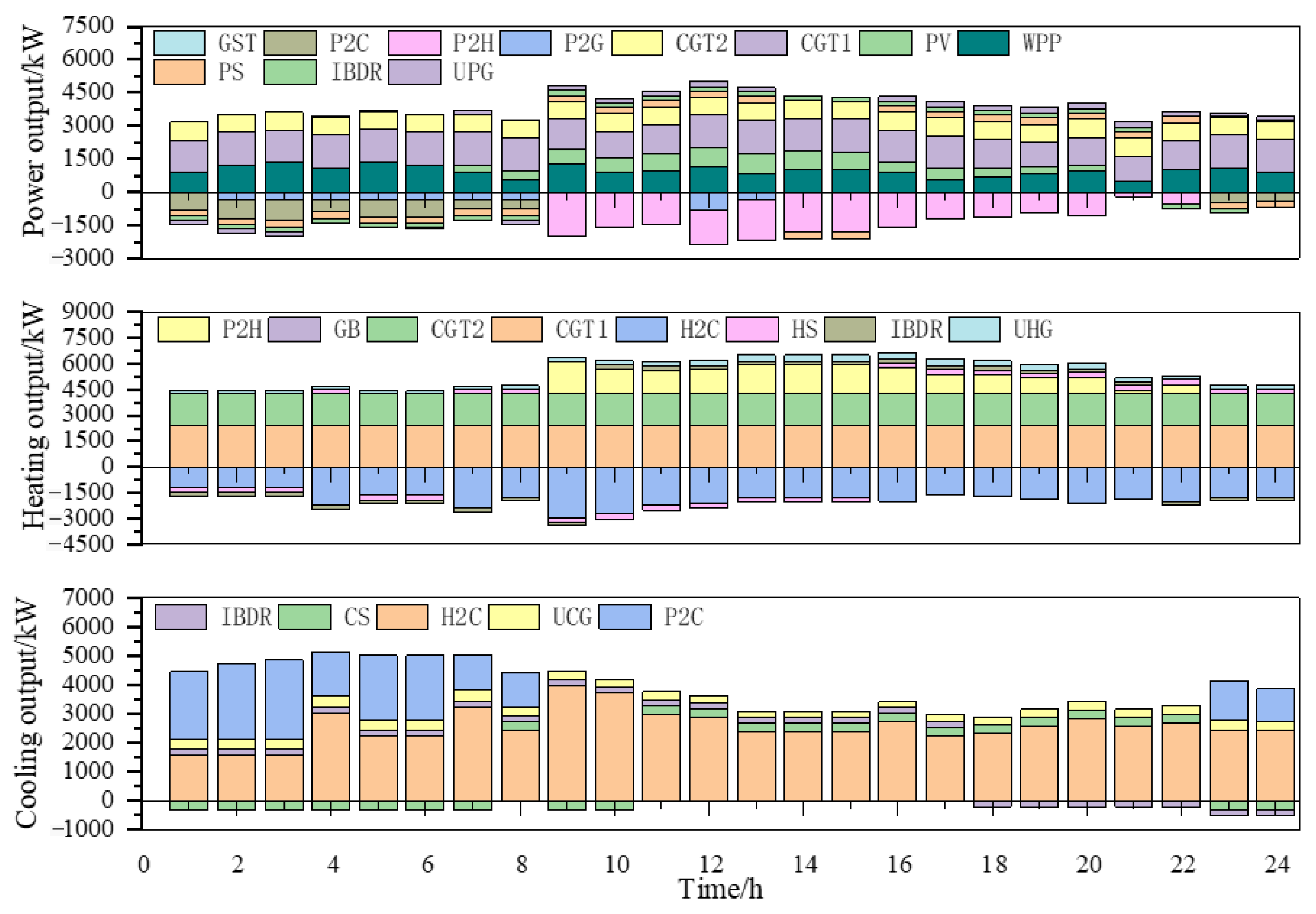
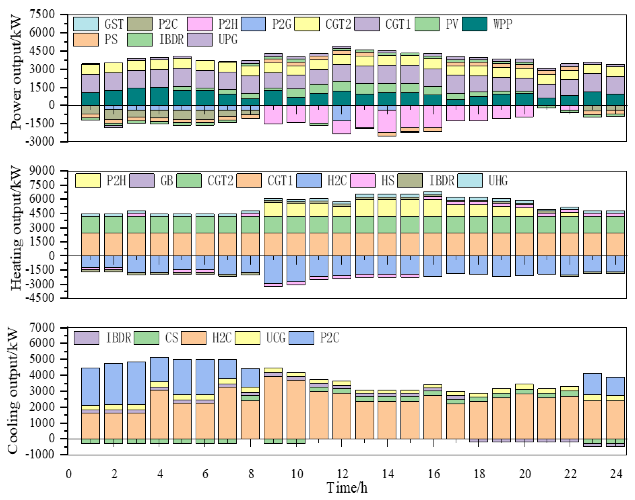
(1) A MES can integrate different types of energy, such as wind, photovoltaics, and gas. Power–gas–heat–cooling (multi-type energy) cycle supply is realized via ECD and ESD to synergistically meet different types of energy demands. In particular, WPP and PV have considerable economic and environmental benefits. Their surplus power can be converted into other types of energy via P2G, P2H, and P2C, after meeting power demands, thus realizing cascade utilization of energy. End users participating in the operation optimization of MES via DR realize source–load interaction.

(2) The constructed multi-objective coordinated dispatching optimization model gives consideration to operating revenue, carbon emissions, and operational risk, and the solution algorithm can be used to obtain an optimal balanced strategy for multiple objectives. The objective values of multi-objective comprehensive optimization are close to the mean values of different single-objective optimization scenarios. Since the weight of the operating revenue objective function is the highest, the operational results are biased towards this objective, which indicates that the dispatching strategy of MES is more balanced.

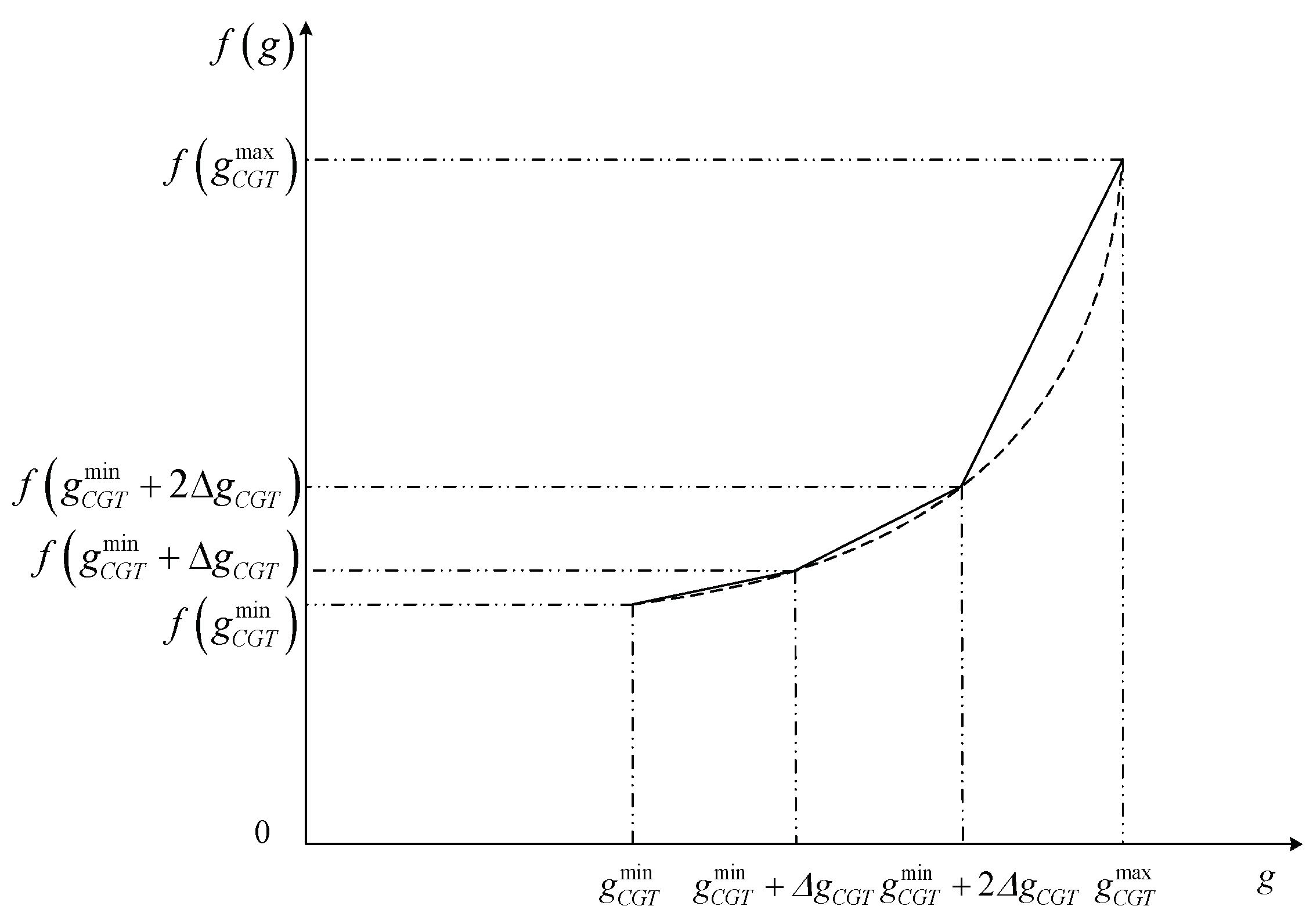
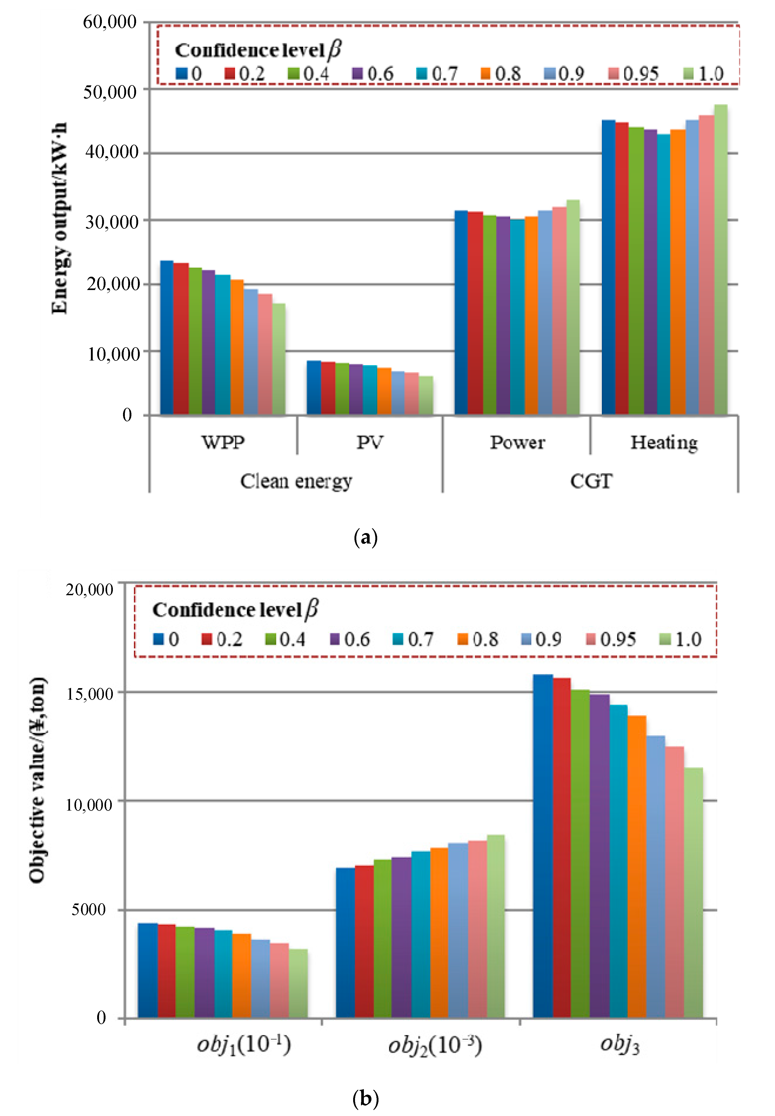
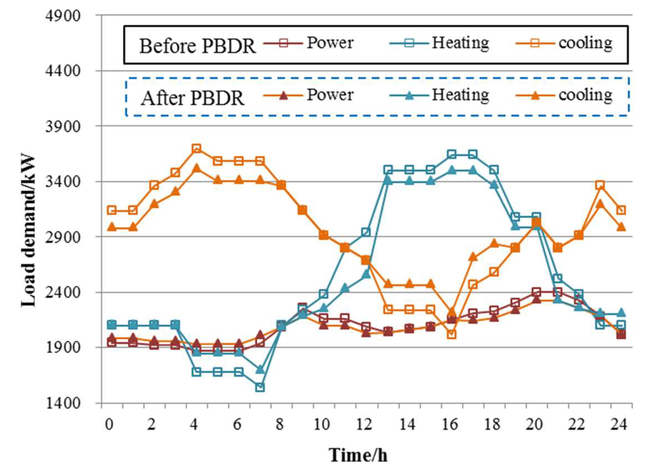
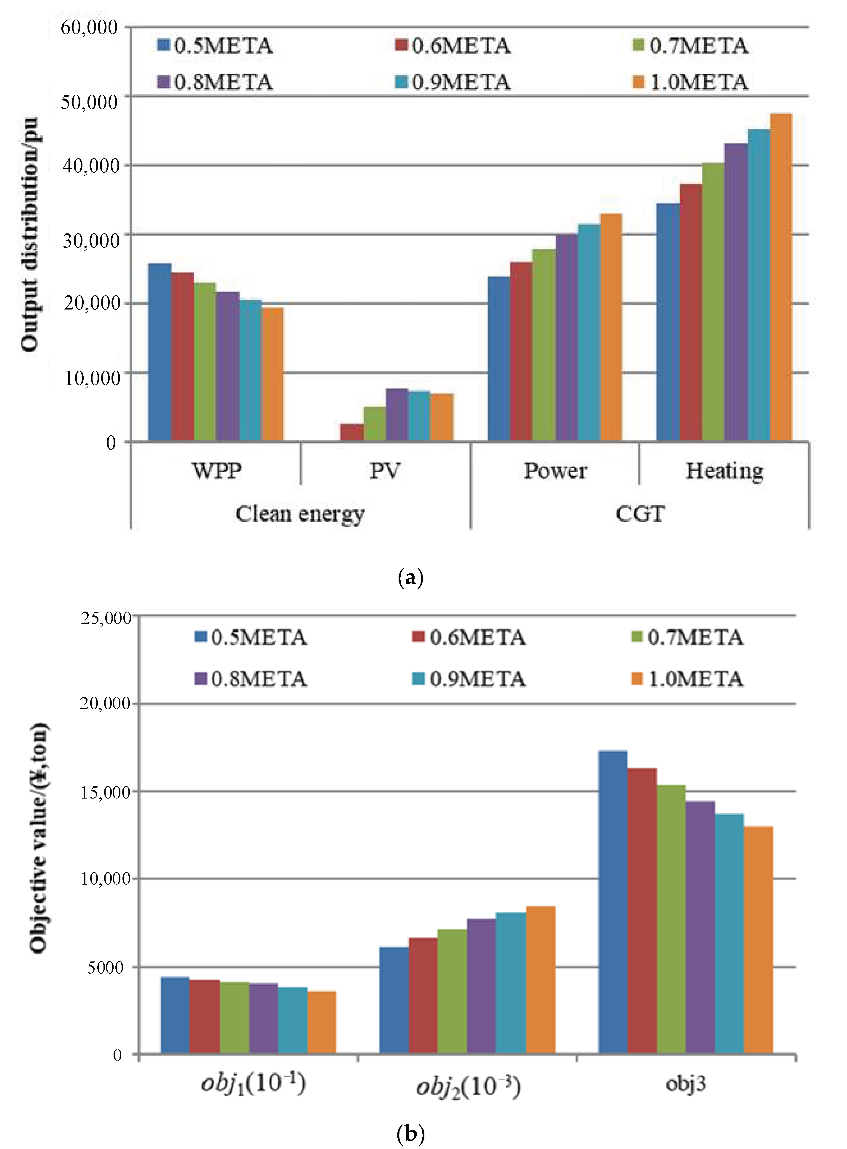
(3) Sensitivity analysis results indicate that a reasonable confidence setting is an effective tool for different decision makers to make dispatching strategies for different interests, and PBDR and MTEA are indirect factors that affect the energy supply structure of a MES. A decision maker prefers risks when the confidence is less than 0.6; confidence within (0.7,0.85) indicates a decision maker is sensitive to risks; and a risk averter, who refuses to take any risks, is indicated by confidence of 0.95 or higher. PBDR is introduced to smooth load curves. MTEA limits energy supplies of CGT, GB, and UEG to increase the chances for WPP and PV on-grid connection, thus optimizing the energy supply structure of the MES.

References

1. Rifkin, J. The Third Industrial Revolution: How Lateral Power is Transforming Energy, the Economy, and the World; Palgrave Macmillan: New York, NY, USA, 2011. [Google Scholar]
2. Liu, Y.; Zuo, K.; Liu, X.; Liu, J.; Kennedy, J.M. Dynamic pricing for decentralized energy trading in micro-grids. Appl. Energy 2018, 228, 689–699. [Google Scholar] [CrossRef]
3. Zhao, X.; Yang, L.; Qu, X.; Yan, W. An improved energy flow calculation method for integrated electricity and natural gas system. Trans. Chin. Electrotech. Soc. 2018, 33, 467–477. [Google Scholar]
4. Ju, L.; Li, H.; Zhao, J.; Chen, K.; Tan, Q.; Tan, Z. Multi-objective stochastic scheduling optimization model for connecting a virtual power plant to wind-photovoltaic-electric vehicles considering uncertainties and demand response. Energy Convers. Manag. 2016, 128, 160–177. [Google Scholar] [CrossRef]
5. Muhammad, F.Z.; Elhoussin, E.; Mohamed, B. Microgrids energy management systems: A critical review on methods, solutions, and prospects. Appl. Energy 2018, 222, 1033–1055. [Google Scholar]
6. Al-Zakwani, S.S.; Maroufmashat, A.; Mazouz, A.; Fowler, M.; Elkamel, A. Allocation of Ontario’s Surplus Electricity to Different Power-to-Gas Applications. Energies 2019, 12, 2675. [Google Scholar] [CrossRef]
7. Zhang, X.; Yang, J.; Wang, W.; Zhang, M.; Jing, T. Integrated Optimal Dispatch of a Rural Micro-Energy-Grid with Multi-Energy Stream Based on Model Predictive Control. Energies 2018, 11, 3439. [Google Scholar] [CrossRef]
8. Anna, L.B.; Umberto, D. Opportunities of power-to-gas technology in different energy systems architectures. Appl. Energy 2018, 228, 57–67. [Google Scholar]
9. Heredia, F.J.; Rider, M.J.; Corchero, C. Optimal Bidding Strategies for Thermal and Generic Programming Units in the Day-Ahead Electricity Market. IEEE Trans. Power Syst. 2010, 25, 1504–1518. [Google Scholar] [CrossRef]
10. Zamani, A.G.; Zakariazadeh, A.; Jadid, S. Day-ahead resource scheduling of a renewable energy based virtual power plant. Appl. Energy 2016, 169, 324–340. [Google Scholar] [CrossRef]
11. Yang, H.; Yi, D.; Zhao, J.; Luo, F.; Dong, Z. Distributed optimal dispatch of virtual power plant based on ELM transformation. J. Ind. Manag. Optim. 2014, 10, 1297–1318. [Google Scholar] [CrossRef]
12. Mohammadi, J.; Rahimikian, A.; Ghazizadeh, M.S. Aggregated wind power and flexible load offering strategy. IET Renew. Power Gener. 2007, 5, 439–447. [Google Scholar] [CrossRef]
13. Wang, H.; Huang, Q.; Zhang, C.; Xia, A. A novel approach for the layout of electric vehicle charging station. In Proceedings of the International Conference on Apperceiving Computing and Intelligence Analysis, Chengdu, China, 17–19 December 2010; pp. 64–70. [Google Scholar]
14. Tan, Z.-F.; Ju, L.-W.; Li, H.-H.; Li, J.-Y.; Zhang, H.-J. A two-stage scheduling optimization model and solution algorithm for wind power and energy storage system considering uncertainty and demand response. Int. J. Electr. Power Energy Syst. 2014, 63, 1057–1069. [Google Scholar] [CrossRef]
15. Jiang, Y.-W.; Chen, C.; Wen, B.-Y. Application of Stochastic Simulation’s Particle Swarm Algorithm in the Compensation of Reactive Power for Wind Farms. Proc. CSEE 2008, 28, 47–52. [Google Scholar]
16. Wang, X.; Wang, X.; LI, L.-X.; Zheng, Y.-H.; Xu, Q.-S. Reactive power optimization for wind power system based on dynamic cloud evolutionary particle swarm optimization. Power Syst. Prot. Control 2013, 41, 36–43. [Google Scholar]
17. Ju, L.; Zhao, R.; Tan, Q.; Lu, Y.; Tan, Q.; Wang, W. A multi-objective robust scheduling model and solution algorithm for a novel virtual power plant connected with power-to-gas and gas storage tank considering uncertainty and demand response. Appl. Energy 2019, 250, 1336–1355. [Google Scholar] [CrossRef]
18. Liu, F.; Zhang, K.; Zou, R. Robust LFC Strategy for Wind Integrated Time-Delay Power System Using EID Compensation. Energies 2019, 12, 3223. [Google Scholar] [CrossRef]
19. Tan, Z.; Wang, G.; Ju, L.; Tan, Q.; Yang, W. Application of CVaR risk aversion approach in the dynamical scheduling optimization model for virtual power plant connected with wind-photovoltaic-energy storage system with uncertainties and demand response. Energy 2017, 124, 198–213. [Google Scholar] [CrossRef]
20. Ju, L.; Zuo, X.; Tan, Q.; Zhao, R.; Wang, W. A risk aversion optimal model for microenergy grid low carbon-oriented operation considering power-to-gas and gas storage tank. Int. J. Energy Res. 2019, 43, 5506–5525. [Google Scholar] [CrossRef]
21. Stojiljkovic, M.M. Bi-level multi-objective fuzzy design optimization of energy supply systems aided by problem-specific heuristics. Energy 2017, 137, 1231–1251. [Google Scholar] [CrossRef]
22. Ju, L.; Tan, Z.; Li, H.; Tan, Q.; Yu, X.; Song, X. Multi-objective operation optimization and evaluation model for CCHP and renewable energy based hybrid energy system driven by distributed energy resources in China. Energy 2016, 111, 322–340. [Google Scholar] [CrossRef] [Green Version]
Figure 1. Structure of the micro energy system micro energy system (MES).
Energies 12 04414 g001
Figure 2. Semi-linear membership function (a) and semi-gradient membership function (b).
Energies 12 04414 g002
Figure 3. The linearization process.
Energies 12 04414 g003
Figure 4. Solving process of multi-objective functions.
Energies 12 04414 g004
Figure 5. Load demands (a) and prices of power, heating, and cooling (b) on a typical day.
Energies 12 04414 g005
Figure 6. Available outputs of the wind power plants (WPP) and photovoltaic plants (PV) on a typical day.
Energies 12 04414 g006
Figure 7. Output distribution based on the maximum operating revenue.
Energies 12 04414 g007
Figure 8. Output distribution based on the minimum carbon emissions.
Energies 12 04414 g008
Figure 9. Output distribution based on the minimum operational risk.
Energies 12 04414 g009
Figure 10. Output distribution based on the comprehensive objective function.
Energies 12 04414 g010
Figure 11. The outputs (a) and objective values (b) under different confidence levels β.
Energies 12 04414 g011
Figure 12. Power, heating, and cooling demands before and after the price-based demand–response (PBDR).
Energies 12 04414 g012
Figure 13. Output distribution after the price-based demand response (PBDR).
Energies 12 04414 g013
Figure 14. Outputs (a) and objective values (b) under different maximum total emission allowance (MTEA) values.
Energies 12 04414 g014