Simulated Annealing Algorithm for Wind Farm Layout Optimization: A Benchmark Study

Abstract
1. Introduction
2. Methodology
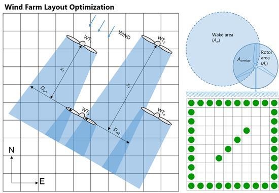
2.1. Wake Model
2.2. Cost Model and Objective Function
2.3. Wind Farm and Wind Scenarios
2.4. Optimization Methodology
| Algorithm 1. Pseudocode of Simulated Annealing for the Wind Farm Layout Optimization. | |
| Input: | Problem size, Initial temperature (T), Stopping temperature (Tmin) |
| Temperature control (α), Number of iteration (Markov number) | |
| 1: | Lcurrent = create(Problem size) // Create and initialize layout of wind turbines |
| 2: | Lbest = Lcurrent |
| 3: | while T > Tmin do |
| 4: | for i = 1 to Markov number do |
| 5: | Li = perturbation(Lcurrent) // Perturbation of wind turbine position |
| 6: | Δcost = cost(Li) − cost(Lcurrent) // Evaluation of cost |
| 7: | if Δcost < 0 then Lcurrent = Li |
| 8: | if cost(Lcurrent) < cost(Lbest) then |
| 9: | Lbest = Lcurrent |
| 10: | end if |
| 11: | else if exp(−Δcost/T) > random then // Metropolis criterion |
| 12: | Lcurrent = Li |
| 13: | end if |
| 14: | end for |
| 15: | T = αT // Decreasing temperature |
| 16: | end while |
| Output: Best layout of wind turbines (Lbest) | |
3. Case Studies and Discussion
3.1. Case Study (a): Constant Wind Speed and Single Wind Direction
3.2. Case Study (b): Constant Wind Speed and Multiple Wind Directions
3.3. Case Study (c): Variable Wind Speed and Multiple Wind Directions
4. Conclusions
Author Contributions
Funding
Conflicts of Interest
References
- Herbert-Acero, J.; Probst, O.; Réthoré, P.-E.; Larsen, G.; Castillo-Villar, K. A Review of Methodological Approaches for the Design and Optimization of Wind Farms. Energies 2014, 7, 6930–7016. [Google Scholar] [CrossRef]
- Shakoor, R.; Hassan, M.Y.; Raheem, A.; Wu, Y.K. Wake effect modeling: A review of wind farm layout optimization using Jensen’s model. Renew. Sustain. Energy Rev. 2016, 58, 1048–1059. [Google Scholar] [CrossRef]
- Mosetti, G.; Poloni, C.; Diviacco, B. Optimization of wind turbine positioning in large windfarms by means of a genetic algorithm. J. Wind Eng. Ind. Aerodyn. 1994, 51, 105–116. [Google Scholar] [CrossRef]
- Grady, S.A.; Hussaini, M.Y.; Abdullah, M.M. Placement of wind turbines using genetic algorithms. Renew. Energy 2005, 30, 259–270. [Google Scholar] [CrossRef]
- Castro Mora, J.; Calero Barón, J.M.; Riquelme Santos, J.M.; Burgos Payán, M. An evolutive algorithm for wind farm optimal design. Neurocomputing 2007, 70, 2651–2658. [Google Scholar] [CrossRef]
- Elkinton, C.N.; Manwell, J.F.; McGowan, J.G. Algorithms for Offshore Wind Farm Layout Optimization. Wind Eng. 2008, 32, 67–84. [Google Scholar] [CrossRef]
- Emami, A.; Noghreh, P. New approach on optimization in placement of wind turbines within wind farm by genetic algorithms. Renew. Energy 2010, 35, 1559–1564. [Google Scholar] [CrossRef]
- González, J.S.; Gonzalez Rodriguez, A.G.; Mora, J.C.; Santos, J.R.; Payan, M.B. Optimization of wind farm turbines layout using an evolutive algorithm. Renew. Energy 2010, 35, 1671–1681. [Google Scholar] [CrossRef]
- Changshui, Z.; Guangdong, H.; Jun, W. A fast algorithm based on the submodular property for optimization of wind turbine positioning. Renew. Energy 2011, 36, 2951–2958. [Google Scholar] [CrossRef]
- Chen, Y.; Li, H.; Jin, K.; Song, Q. Wind farm layout optimization using genetic algorithm with different hub height wind turbines. Energy Convers. Manag. 2013, 70, 56–65. [Google Scholar] [CrossRef]
- Rahbari, O.; Vafaeipour, M.; Fazelpour, F.; Feidt, M.; Rosen, M.A. Towards realistic designs of wind farm layouts: Application of a novel placement selector approach. Energy Convers. Manag. 2014, 81, 242–254. [Google Scholar] [CrossRef]
- Gao, X.; Yang, H.; Lin, L.; Koo, P. Wind turbine layout optimization using multi-population genetic algorithm and a case study in Hong Kong offshore. J. Wind Eng. Ind. Aerodyn. 2015, 139, 89–99. [Google Scholar] [CrossRef]
- Mayo, M.; Daoud, M. Informed mutation of wind farm layouts to maximise energy harvest. Renew. Energy 2016, 89, 437–448. [Google Scholar] [CrossRef]
- Yamani Douzi Sorkhabi, S.; Romero, D.A.; Yan, G.K.; Gu, M.D.; Moran, J.; Morgenroth, M.; Amon, C.H. The impact of land use constraints in multi-objective energy-noise wind farm layout optimization. Renew. Energy 2016, 85, 359–370. [Google Scholar] [CrossRef]
- Wang, L.; Cholette, M.E.; Tan, A.C.C.; Gu, Y. A computationally-efficient layout optimization method for real wind farms considering altitude variations. Energy 2017, 132, 147–159. [Google Scholar] [CrossRef]
- Pillai, A.C.; Chick, J.; Khorasanchi, M.; Barbouchi, S.; Johanning, L. Application of an offshore wind farm layout optimization methodology at Middelgrunden wind farm. Ocean. Eng. 2017, 139, 287–297. [Google Scholar] [CrossRef]
- Song, M.; Wen, Y.; Duan, B.; Wang, J.; Gong, Q. Micro-siting optimization of a wind farm built in multiple phases. Energy 2017, 137, 95–103. [Google Scholar] [CrossRef]
- Kirchner-Bossi, N.; Porté-Agel, F. Realistic wind farm layout optimization through genetic algorithms using a Gaussian wake model. Energies 2018, 11, 3268. [Google Scholar] [CrossRef]
- Parada, L.; Herrera, C.; Flores, P.; Parada, V. Wind farm layout optimization using a Gaussian-based wake model. Renew. Energy 2017, 107, 531–541. [Google Scholar] [CrossRef]
- Kusiak, A.; Song, Z. Design of wind farm layout for maximum wind energy capture. Renew. Energy 2010, 35, 685–694. [Google Scholar] [CrossRef]
- Kusiak, A.; Zheng, H. Optimization of wind turbine energy and power factor with an evolutionary computation algorithm. Energy 2010, 35, 1324–1332. [Google Scholar] [CrossRef]
- Song, Z.; Zhang, Z.; Chen, X. The decision model of 3-dimensional wind farm layout design. Renew. Energy 2016, 85, 248–258. [Google Scholar] [CrossRef]
- Chowdhury, S.; Zhang, J.; Messac, A.; Castillo, L. Unrestricted wind farm layout optimization (UWFLO): Investigating key factors influencing the maximum power generation. Renew. Energy 2012, 38, 16–30. [Google Scholar] [CrossRef]
- Pookpunt, S.; Ongsakul, W. Optimal placement of wind turbines within wind farm using binary particle swarm optimization with time-varying acceleration coefficients. Renew. Energy 2013, 55, 266–276. [Google Scholar] [CrossRef]
- Hou, P.; Hu, W.; Chen, C.; Soltani, M.; Chen, Z. Optimization of offshore wind farm layout in restricted zones. Energy 2016, 113, 487–496. [Google Scholar] [CrossRef]
- Ozturk, U.A.; Norman, B.A. Heuristic methods for wind energy conversion system positioning. Electr. Power Syst. Res. 2004, 70, 179–185. [Google Scholar] [CrossRef]
- Chen, K.; Song, M.X.; Zhang, X.; Wang, S.F. Wind turbine layout optimization with multiple hub height wind turbines using greedy algorithm. Renew. Energy 2016, 96, 676–686. [Google Scholar] [CrossRef]
- Marmidis, G.; Lazarou, S.; Pyrgioti, E. Optimal placement of wind turbines in a wind park using Monte Carlo simulation. Renew. Energy 2008, 33, 1455–1460. [Google Scholar] [CrossRef]
- Rivas, R.A.; Clausen, J.; Hansen, K.S.; Jensen, L.E. Solving the Turbine Positioning Problem for Large Offshore Wind Farms by Simulated Annealing. Wind Eng. 2009, 33, 287–297. [Google Scholar] [CrossRef]
- Eroĝlu, Y.; Seçkiner, S.U. Design of wind farm layout using ant colony algorithm. Renew. Energy 2012, 44, 53–62. [Google Scholar] [CrossRef]
- Kallioras, N.A.; Lagaros, N.D.; Karlaftis, M.G.; Pachy, P. Optimum layout design of onshore wind farms considering stochastic loading. Adv. Eng. Softw. 2015, 88, 8–20. [Google Scholar] [CrossRef]
- DuPont, B.; Cagan, J.; Moriarty, P. An advanced modeling system for optimization of wind farm layout and wind turbine sizing using a multi-level extended pattern search algorithm. Energy 2016, 106, 802–814. [Google Scholar] [CrossRef]
- Wagner, M.; Day, J.; Neumann, F. A fast and effective local search algorithm for optimizing the placement of wind turbines. Renew. Energy 2013, 51, 64–70. [Google Scholar] [CrossRef]
- Archer, R.; Nates, G.; Donovan, S.; Waterer, H. Wind Turbine Interference in a Wind Farm Layout Optimization Mixed Integer Linear Programming Model. Wind Eng. 2011, 35, 165–175. [Google Scholar] [CrossRef]
- Turner, S.D.O.; Romero, D.A.; Zhang, P.Y.; Amon, C.H.; Chan, T.C.Y. A new mathematical programming approach to optimize wind farm layouts. Renew. Energy 2014, 63, 674–680. [Google Scholar] [CrossRef]
- Kuo, J.Y.J.; Romero, D.A.; Amon, C.H. A mechanistic semi-empirical wake interaction model for wind farm layout optimization. Energy 2015, 93, 2157–2165. [Google Scholar] [CrossRef]
- MirHassani, S.A.; Yarahmadi, A. Wind farm layout optimization under uncertainty. Renew. Energy 2017, 107, 288–297. [Google Scholar] [CrossRef]
- Park, J.; Law, K.H. Layout optimization for maximizing wind farm power production using sequential convex programming. Appl. Energy 2015, 151, 320–334. [Google Scholar] [CrossRef]
- Guirguis, D.; Romero, D.A.; Amon, C.H. Toward efficient optimization of wind farm layouts: Utilizing exact gradient information. Appl. Energy 2016, 179, 110–123. [Google Scholar] [CrossRef]
- Tingey, E.B.; Ning, A. Trading off sound pressure level and average power production for wind farm layout optimization. Renew. Energy 2017, 114, 547–555. [Google Scholar] [CrossRef]
- King, R.N.; Dykes, K.; Graf, P.; Hamlington, P.E. Optimization of wind plant layouts using an adjoint approach. Wind Energy Sci. 2017, 2, 115–131. [Google Scholar] [CrossRef]
- Du, K.L.; Swamy, M.N.S. Search and optimization by metaheuristics: Techniques and algorithms inspired by nature. In Search Optimization by Metaheuristics Techniques Algorithms Inspired by Nature; Birkhäuser: Basel, Switzerland, 2016; pp. 1–434. [Google Scholar]
- Jensen, N.O. A Note on Wind Generator Interaction; Technical; Risø National Laboratory: Roskilde, Denmark, 1983. [Google Scholar]
- Katic, I.; Højstrup, J.; Jensen, N.O. A Simple Model for Cluster Efficiency. In Proceedings of the European Wind Energy Association Conference and Exhibition, Rome, Italy, 7–9 October 1986; pp. 407–410. [Google Scholar]
- Brownlee, J. Clever Algorithms Nature-Inspired Programming Recipes, 1st ed.; Lulu Press: Morrisville, NC, USA, 2011; ISBN 9781446785065. [Google Scholar]
- Yang, K.; Kwak, G.; Cho, K.; Huh, J. Wind farm layout optimization for wake effect uniformity. Energy 2019, 183, 983–995. [Google Scholar] [CrossRef]


| Property | Value | Property | Value |
|---|---|---|---|
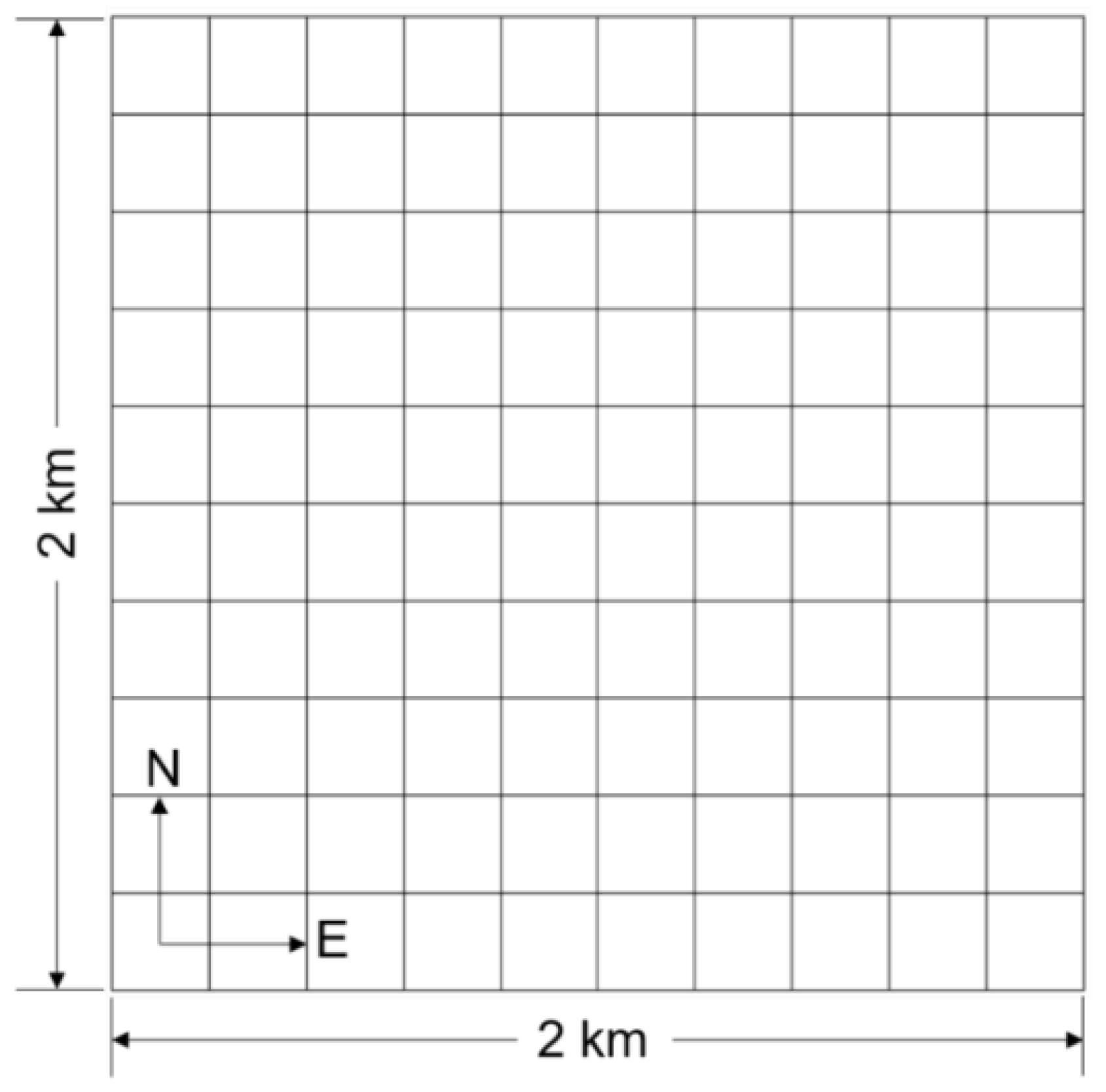
| Hub height (h) | 60 m | Wind farm size | 2 × 2 km |
| Rotor diameter (D) | 40 m | Surface roughness length (z0) | 0.3 m |
| Thrust coefficient (Ct) | 0.88 | Air density (ρ) | 1.225 kg/m3 |
| Power coefficient (Cp) | 0.39 | Spacing | 200 m (5D) |
| Axial induction factor (a) | 0.326 | Entrainment constant (α) | 0.094 |
| Parameter | Value | Parameter | Value |
|---|---|---|---|
| Number of cells | 10 × 10 | Initial temperature | 1.0 |
| Cell size | 200 × 200 m | Stopping temperature | 0.001 |
| Markov number | 200 | Temperature control (α) | 0.98 |
| Number of Turbines | Total Power (kW) | Efficiency (%) | Fitness Value | |
|---|---|---|---|---|
| Mosetti et al. [3] | 26 | 12,349 (12,352) | 91.621 (91.645) | 0.0016201 (0.0016197) |
| Grady et al. [4] | 30 | 14,269 (14,310) | 91.756 (92.015) | 0.0015479 (0.0015436) |
| González et al. [8] | 30 | 14,269 (not reported) | 91.756 (−) | 0.0015479 (−) |
| Parada et al. [19] | 30 | 14,269 (14,785) | 91.756 (95.068) | 0.0015479 (0.0014940) |
| Zhang et al. [9] | 30 | 14,269 (14,310) | 91.756 (92.015) | 0.0015479 (0.0015436) |
| Present study | 30 | 14,269 | 91.756 | 0.0015479 |
| Number of Turbines | Total Power (kW) | Efficiency (%) | Fitness Value | |
|---|---|---|---|---|
| Mosetti et al. [3] | 19 | 9216 (9244) | 93.570 (93.859) | 0.0017411 (0.0017371) |
| Grady et al. [4] | 39 | 17,420 (17,220) | 86.165 (85.174) | 0.0015454 (0.0015666) |
| González et al. [8] | 39 | 17,415 (18,065) | 86.141 (89.353) | 0.0015458 (0.0014903) |
| Parada et al. [19] | 39 | 17,526 (18,866) | 86.688 (93.315) | 0.0015361 (0.0014270) |
| Zhang et al. [9] | 40 | 17,709 (17,991) | 85.404 (86.762) | 0.0015523 (0.0015280) |
| Present study | 40 | 18,244 | 87.983 | 0.0015068 |
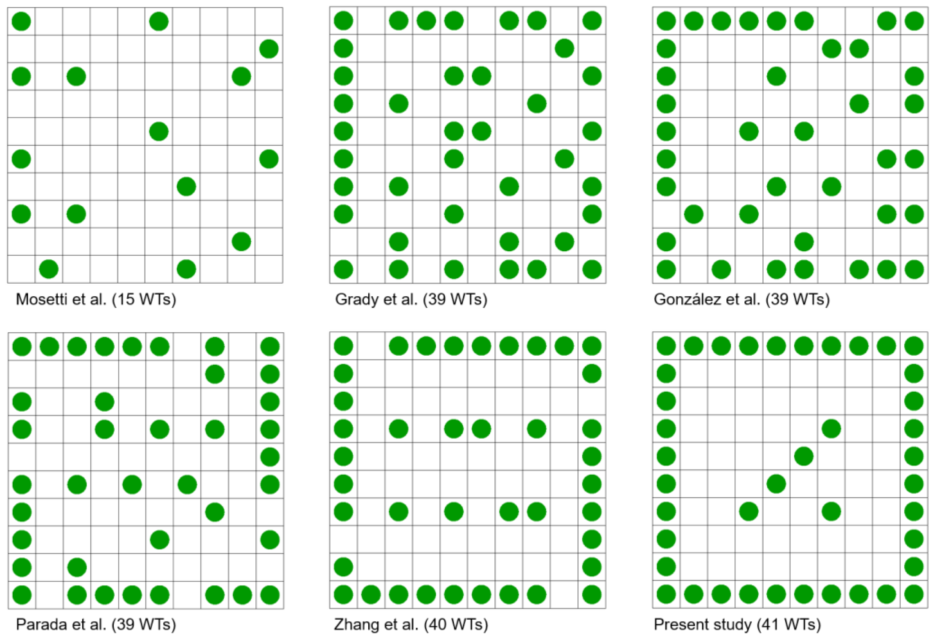
| Number of Turbines | Total Power (kW) | Efficiency (%) | Fitness Value | |
|---|---|---|---|---|
| Mosetti et al. [3] | 15 | 13,319 (13,460) | 94.656 (94.620) | 0.0010046 (0.0009941) |
| Grady et al. [4] | 39 | 31,636 (32,038) | 86.471 (86.619) | 0.0008510 (0.0008403) |
| González et al. [8] | 39 | 31,984 (32,739) | 87.177 (89.487) | 0.0008441 (0.0008223) |
| Parada et al. [19] | 39 | 31,862 (34,173) | 87.089 (93.407) | 0.0008449 (0.0007878) |
| Zhang et al. [9] | 40 | 32,868 (34,271) | 87.593 (91.333) | 0.0008364 (0.0008022) |
| Present study | 41 | 33,966 | 88.311 | 0.0008263 |
© 2019 by the authors. Licensee MDPI, Basel, Switzerland. This article is an open access article distributed under the terms and conditions of the Creative Commons Attribution (CC BY) license (http://creativecommons.org/licenses/by/4.0/).
Share and Cite
Yang, K.; Cho, K. Simulated Annealing Algorithm for Wind Farm Layout Optimization: A Benchmark Study. Energies 2019, 12, 4403. https://doi.org/10.3390/en12234403
Yang K, Cho K. Simulated Annealing Algorithm for Wind Farm Layout Optimization: A Benchmark Study. Energies. 2019; 12(23):4403. https://doi.org/10.3390/en12234403
Chicago/Turabian StyleYang, Kyoungboo, and Kyungho Cho. 2019. "Simulated Annealing Algorithm for Wind Farm Layout Optimization: A Benchmark Study" Energies 12, no. 23: 4403. https://doi.org/10.3390/en12234403
APA StyleYang, K., & Cho, K. (2019). Simulated Annealing Algorithm for Wind Farm Layout Optimization: A Benchmark Study. Energies, 12(23), 4403. https://doi.org/10.3390/en12234403