Abstract
Wake models play an integral role in wind farm layout optimization and operations where associated design and control decisions are only as good as the underlying wake model upon which they are based. However, the desired model fidelity must be counterbalanced by the need for simplicity and computational efficiency. As a result, efficient engineering models that accurately capture the relevant physics—such as wake expansion and wake interactions for design problems and wake advection and turbulent fluctuations for control problems—are needed to advance the field of wind farm optimization. In this paper, we discuss a computationally-efficient continuous-time one-dimensional dynamic wake model that includes several features derived from fundamental physics, making it less ad-hoc than prevailing approaches. We first apply the steady-state solution of the model to predict the wake expansion coefficients commonly used in design problems. We demonstrate that more realistic results can be attained by linking the wake expansion rate to a top-down model of the atmospheric boundary layer, using a super-Gaussian wake profile that smoothly transitions between a top-hat and Gaussian distribution as well as linearly-superposing wake interactions. We then apply the dynamic model to predict trajectories of wind farm power output during start-up and highlight the improved accuracy of non-linear advection over linear advection. Finally, we apply the dynamic model to the control-oriented application of predicting power output of an irregularly-arranged farm during continuous operation. In this application, model fidelity is improved through state and parameter estimation accounting for spanwise inflow inhomogeneities and turbulent fluctuations. The proposed approach thus provides a modeling paradigm with the flexibility to enable designers to trade-off between accuracy and computational speed for a wide range of wind farm design and control applications.
1. Introduction
Improving wind farm design and control is at the core of wind energy research aimed at facilitating greater wind energy penetration. Design problems focus on maximizing wind farm power production and reducing the levelized cost of energy by optimizing wind farm layouts [1,2,3,4] and wind turbine set points for yaw, tilt, and thrust [5,6]. Active control attempts to actuate turbines dynamically to reduce farm level power fluctuations [7], track a power output reference signal to provide power grid services [8,9,10,11], or maximize power production [12,13].
Design and control studies rely on engineering models that can be easily computed and optimized because high-fidelity simulations are too computationally expensive to be practical. Traditional engineering design models focus on wake growth rates, the shape of the velocity deficit in the transverse directions downstream of the turbine (the wake profile), and wake interactions. However, the details and capabilities of these models vary considerably. For example, the wake profile shape can be modeled as a top-hat [14,15], Gaussian [16,17], or a more complicated step-wise function [18]. Wake areas are often modeled as growing linearly with downstream distance [14,15], but have also been represented with other functional forms [19]. Velocity deficits arising from wake interactions may be computed as a linear sum [20,21] or as a sum of squares [14,15]. Related modeling approaches include the effects of the atmospheric boundary layer (ABL) on the wind turbine array through one-way [22] or two-way coupling [23,24] with ABL models [19,25,26]. Design-related models may also include certain dynamic effects such as yaw and tilt actuation [27,28,29] or the turbulent meandering of wakes [30]. These design models are typically either static or account for limited temporal variations and therefore cannot capture changing wind farm conditions or power output levels.
Active and closed-loop control applications, on the other hand, require time-dependent models that can capture the effects of control actions. Dynamic modeling approaches also vary considerably in fidelity, modeling philosophy, and underlying assumptions. The simplest models are discrete-time extensions of steady-state wake models [31] and continuous-time one-dimensional models [8,32]. Higher fidelity, yet more computationally-expensive, models include two-dimensional Reynolds-averaged Navier–Stokes (RANS) simulations [33] and very coarse large-eddy simulations (LES) [34].
Design and control-oriented models also differ in their implementation. In design problems, the goal is to estimate the effect of wind turbines on the fluid flow prior to implementation or construction of the farm. Therefore, steady-state model coefficients cannot be directly measured and are instead estimated empirically [20,21,35] based on site-specific data, or more infrequently, via physics-based methods [24]. In closed-loop control applications, parameter estimation is enabled through real-time data regarding power output or from flow field sensors that provide a means of fitting model coefficients to local site-specific attributes based on the current flow state [4,36,37].
In other ways, dynamic models have a range of complications that are not relevant to steady-state models. For example, the temporal effect of large-scale turbulent structures and the non-linearity of advection affect inter-turbine travel times. These interactions impact the instantaneous power output of individual turbines within a farm, but may not change the time-averaged power output. Therefore, these effects have not been extensively discussed in studies that focus on steady-state applications.
In this paper, we build on our previously-proposed continuous-time one-dimensional dynamic wake model [32] to provide a unified modeling framework for steady-state design and active control applications. We demonstrate how the selection of modeling parameters, including the wake mixing and expansion model, the wake profile shape, the advection scheme, and the inflow model, can improve model fidelity. For the dynamic model, we introduce a filtering approach to incorporate spanwise inhomogeneity in the inlet conditions to improve the inflow model, as well as state and parameter estimation to improve power output prediction. We then demonstrate that these estimation techniques can correct model errors, such as those introduced when using a linear advection model.
The remainder of this paper is organized as follows. We introduce the model proposed in [8] in Section 2, along with a new definition of the wake profile that improves the model accuracy. In Section 3, we discuss how to parameterize the model for design applications that employ the steady-state version of the model, where improved performance is achieved by linking the wake expansion rates to top-down atmospheric models [26]. In Section 4, we apply the dynamic model to a range of problems starting with the prediction of the power trajectory of a wind farm at start-up. We then introduce measurement-based state and parameter estimation approaches to account for spanwise inhomogeneities in the inlet and modeling errors. Finally, we summarize and discuss the conclusions in Section 5.
2. Wake Model
This paper builds on the dynamic wake model introduced in [8] and extended to include the effect of yaw in [32]. The model presented here differs from previous versions in the following ways. Velocity deficits are linearly superposed; the wake growth rate is linked to the friction velocity; and the wake profile model incorporates a smooth transition from a top-hat to a Gaussian wake profile.
We begin by considering a wind farm with N turbines each with diameter . The coordinate system is defined such that x is the streamwise direction, y is the spanwise direction, and z is the vertical direction. The center of the turbine’s rotor is located at . The inflow velocity to the farm may vary in time and space ; however, in some cases, the time-averaged or time- and space-averaged velocity may be the more appropriate, and the arguments of the averaged quantities will be omitted.
The streamwise velocity deficit behind the turbine is governed by the one-dimensional partial differential equation (PDE) (no Einstein summation convention over n is implied):
The advection velocity can be specified is several ways. Here, we focus on two cases: the linear advection model of the form , which was used in [37] for ease of implementation, and the nonlinear form . The function is a normalized Gaussian function with characteristic width R:
The function defines the wake expansion rate as:
which depends on the wake area that is defined in Section 2.1.
The source term is specified by the initial velocity deficit , which is obtained from an inviscid model [14,38]. In the case where the thrust is pointing in the direction of the upstream velocity, the appropriate inviscid model that relies on actuator disk theory [38] gives an initial velocity deficit of:
where is the thrust coefficient and is the upstream velocity at turbine n. The initial velocity deficits can also be described in terms of the local thrust coefficient and the disk-averaged velocity across the turbine rotor .
For the dynamic model, we follow the convention of LES [25,39] and use and in the model. Assuming that the resulting velocity field is consistent under Galilean transformations, we adopt a linear superposition of velocity deficits. The resulting velocity field is found by distributing the velocity deficits using the wake profile defined in Section 2.2 and subtracting the result from the inlet flow velocity :
The linear superposition approach simplifies the implementation within a model-based control framework and agrees well with the data, as shown in Section 3. This disk-averaged velocity for turbine n, , is found by sampling the velocity field according to:
where is the squared radial coordinate of the turbine.
For the steady-state case, it is easier to use and . The corresponding steady-state solution of the dynamic model [32] is:
Linear superposition of the other wakes can be used to find the upstream velocity of each turbine:
2.1. Turbulent Wake Mixing and Expansion
The wake model in Section 2 captures the dynamics of wake advection, inter-turbine wake interactions (through velocity deficit superposition), and the effect of wake growth on the magnitude of the velocity deficit in the wake. A functional form for the wake area , defined using the normalized wake diameter , that properly captures the effect of turbulent mixing of the wake with the surrounding turbulent atmospheric boundary layer is needed to specify the model fully. We now derive the required form for the wake area through the self-similarity assumption applied to the Reynolds-averaged mean momentum equation associated with a turbine in the ABL. For convenience, we dispense with the turbine indexing in this section, and the origin of the coordinate system is placed at the center of the turbine rotor.
After linearizing the advective term, assuming the pressure gradient vanishes in the region sufficiently downstream from the turbine, neglecting the streamwise Reynolds stress, and using the eddy viscosity model, the Reynolds-averaged mean momentum equation for the streamwise velocity u in the region away from the turbine forcing becomes:
where is the eddy viscosity, and we have assumed a constant inflow velocity for the turbine of interest. The far wake of a turbine has been shown empirically to have a self-similar profile [16]; therefore, the velocity may be written as:
where is a self-similar function of and is proportional to the diameter of the wake.
For a free wake, the eddy viscosity scales with the wake width and the velocity deficit [40]. In the atmospheric boundary layer, however, the appropriate velocity scale is the friction velocity , giving the following eddy viscosity:
Substituting (10) and (11) into (9) and expanding the derivatives, we obtain:
where primes denote derivatives with respect to . Rearranging (12) in dimensionless form leads to:
The expression (13) shows that in order for the profile to be self-similar, the following two conditions must hold in the wake:
Integrating (14), we find that , and the wake diameter expands linearly with downstream distance, as in the Jensen model [14,15]. This yields a normalized wake diameter of:
where the wake expansion coefficient:
is proportional to the ratio of the friction velocity and hub-height velocity, validating the empirical suggestion of Frandsen [35]. The parameter will remain as the only free parameter available to the model.
While the solution to (15) only requires , we can find the scaling using momentum flux conservation in the far field limit using:
where C is a constant that depends on the initial velocity deficit in the wake and the integral . Therefore, the velocity deficit scales inversely with the square of the downstream distance . Solving the steady-state version of the PDE (1) also provides this scaling.
While the linear growth rate is valid in the wake region of the turbine, it is ill-posed upstream of the turbine, where it can vanish or become negative. Therefore, we instead use the following modified function [8] that smoothly approximates the linear expansion in the far wake while avoiding becoming less than unity close to the turbine:
Defined this way, the normalized wake diameter specifies the wake expansion rate (3) needed to define the velocity deficit PDE (1) fully.
2.2. Wake Profile
We now propose a new functional form for the wake profile in (5). Experimental observations have revealed that the shape of the wake profile as a function of spanwise distance slowly transitions from a top-hat profile (cf. the left panel of Figure 1) immediately following the rotor disk to a self-similar Gaussian profile farther downstream in the far wake [16,20,28]. For simplicity, the Jensen model traditionally used top-hat profiles for the entire downstream evolution of the wake [14,15], but such profiles poorly describe the far wake profile that dominates the interaction of upstream wakes on downstream turbines. Other models use the Gaussian profile for the entire wake [16], which overestimates the centerline deficit near the turbine, or model the transition from the top-hat as a decaying potential core [28].
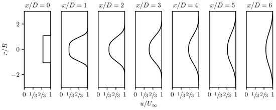
Figure 1.
Profiles of streamwise velocity at various downstream distances based on the wake profile function in (20).
Here, we propose a super-Gaussian function that more accurately approximates the known transition from a top-hat profile to a Gaussian profile. As in Section 2.1, we remove the turbine indexing for convenience and set the origin of the coordinate at the center of the turbine rotor. The proposed wake profile function is of the form:
where is a parameter defining the width of the wake relative to the wake diameter and is a parameter that characterizes the smoothness of the wake. In order to transition from a top-hat profile at the rotor disk to a Gaussian in the far wake, we require that:
Furthermore, should be specified such that the profile becomes nearly Gaussian at [28]. To satisfy these conditions, we define:
where at .
The wake function must also be defined to conserve mass, which means that for a single turbine subject to the inflow velocity :
Alternatively, the integral can be expressed as:
the solution of which [41] (p. 342 #3.478.1) is:
Therefore, the scaling value is:
with and .
The resulting profiles for the velocity in the wake, assuming , and , are shown in Figure 1. These profiles begin as a top-hat with the expected velocity of , at the rotor disk, where a is the induction factor. Around , the velocity is a smoothed top-hat with in the middle of the wake. Further downstream, the deficit decays, transitioning to a Gaussian by mimicking the potential core region noted in [28].
This functional form captures the mean velocity in both the near wake, where the velocity deficit of an actuator disk has a top-hat profile, and the far wake, where the velocity deficit has a Gaussian profile. Small-scale features, such as trailing root and tip vortices, and turbine-specific thrust profiles are not captured by this functional form. In cases where these specifics are deemed important, the functional form can only be assumed to be valid for . With the wake profile specified, the model presented in this section is fully defined with a single free parameter that specifies the wake recovery rate inside the farm.
3. The Steady-State Model for Design Applications
For design problems, we require a method to specify the unknown coefficient for the wake expansion coefficient (17). In typical models, it is obtained using empirical tables based on surface and atmospheric conditions. The recently-proposed coupled wake boundary layer (CWBL) model [23,24,42] eliminates the need for empirical tables by coupling the wake expansion coefficient of the Jensen model to the top-down model [19,25], which provides information about the turbulence characteristics of the wind turbine array boundary layer.
The CWBL determines the single free parameter of the Jensen wake model, the fully-developed wake expansion coefficient , by matching the power prediction of the top-down and Jensen wake model. For a given wake expansion coefficient, the top-down wake model planform thrust coefficient is determined by finding the wake area of the farm; i.e. , where is the planform area of the farm and is the effective wake area coverage. The wake expansion coefficient in the developing region is then assumed to transition from to using a heuristic equation.
Here, we use a related approach, but make several important modifications. First, we replace the Jensen wake model with the steady-state solution of the wake model described above. The remaining differences in the approaches are highlighted in the remainder of this section. Most notably, we dispense with the rather strong assumption of the standard top-down model that the disk-averaged velocity is equal to the planar-averaged hub-height velocity to calculate the planform-averaged thrust coefficient and power production. We represent entrance effects using the developing top-down model [26,43] and replace the heuristic wake growth parameter development with the classic equation for the developing internal boundary layer.
We detail our approach by first introducing the fully-developed top-down model [25]. This model assumes constant stress regions above and below the wind turbine layer, with friction velocities of and and roughness heights of and , respectively. The planar-averaged momentum balance results in the following relationship:
where is the planar-averaged velocity at hub height . Within the wind turbine wake region , where R is the rotor radius, the wind turbine wakes are assumed to generate an additional eddy viscosity . The resulting eddy viscosity in the wake region is below the hub height and above the hub height , where .
Applying momentum conservation and velocity continuity across the layers, the roughness height of the wind farm is:
where . The friction velocities are:
where is the free-stream friction velocity and is the height of the boundary layer. The planar-averaged hub-height velocity is:
In the CWBL model, the disk-averaged velocity is then assumed to be approximately equal to the planar-averaged hub-height velocity to calculate the power production of the farm.
In contrast to the CWBL model, we assume that the top-down model only provides useful predictions of the planar-average hub-height velocity, but not of the individual turbine power, which depends on the more local velocity at each turbine rather than the planar-averaged velocity. As a result, the proper matching condition to find the free parameter of the present model, which scales the wake expansion coefficients as a function of friction velocity, is to require consistency between the planar averaged velocities from the top-down and the wake model. In practice, we find that minimizes the difference between the modeled planar-averaged velocities:
where the superscripts and correspond to the top-down and wake models, respectively.
In order to match the planar-averaged velocity from the wake model corresponding to each turbine, the wind farm’s planform area must be divided into regions that “belong” to each turbine. Here, we propose to use Voronoi tessellation to identify these areas. Difficulties arise at the edge of the farm, where the edge turbines are closest to infinite sections spanning the entire planform area. We address this issue by performing an initial Voronoi tessellation and reflecting each edge turbine across the adjacent line segments of the tessellation to create ghost points. Using the ghost points, Voronoi tessellation is used again to find the planform area of each turbine. The area sections obtained through this algorithm are shown in Figure 2 and Figure 3 for the Horns Rev wind farm and a randomly-generated wind farm, respectively. The left panels show the original Voronoi tessellation with the ghost point projections. The right panels show the final tessellation of the wind farm.
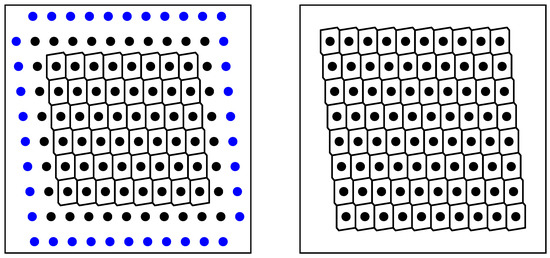
Figure 2.
Voronoi tessellation of the Horns Rev wind farm showing wind turbine locations (black dots), ghost point locations (blue dots), and Voronoi cells (black lines). The left panel shows the original tessellation with ghost point projections. The right panel shows the final tessellation with the ghost points removed.
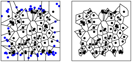
Figure 3.
Voronoi tessellation of a randomly-generated wind farm showing wind turbine locations (black dots), ghost point locations (blue dots), and Voronoi cells (black lines). The left panel shows the original tessellation with ghost point projections. The right panel shows the final tessellation with the ghost points removed.
We model entrance effects using the developing top-down model [26,43], where the boundary transitions from a single log-law profile with surface roughness height to the fully-developed top-down model described above. In the transition region, an internal boundary layer grows from the height of the wind farm at until it reaches the final boundary layer height at . The classical internal boundary layer growth model dictates that:
until . The friction velocities (30) and (31) and planar-averaged velocity (32) evolve with streamwise distance x, where is replaced with the internal boundary layer height .
In our application of the model, the planform thrust coefficient needed for the top-down model is calculated using the force determined by the wake model:
where is the planform area of the Voronoi cell around the turbine. This planform thrust coefficient also provides the surface roughness . Although this value should strictly represent the roughness height of the fully-developed regime, in smaller wind farms, it is difficult to find the roughness height from matching. Therefore, we assume that within each cell, the planform thrust coefficient represents the average coefficient from upstream turbines. Furthermore, the starting location of the internal boundary layer is assumed to coincide with the most upstream turbine, the wake of which, defined by the cone with diameter , intersects the rotor of the turbine.
Using the friction velocities at each turbine, we can determine the wake expansion coefficients that the effective friction velocity at each turbine is the average of the low and high friction velocities , and the advection velocity is the planar-averaged velocity . As a result, the wake expansion coefficient (17), which is the input to the wake model, can be written as:
For a single turbine, this reduces to the expected . This improvement replaces the heuristic development function with a physically-based function and eliminates the difficulty of identifying a fully-developed regime to determine the effective wake area coverage that is needed in the CWBL approach.
We validate our proposed steady state model by applying it to the Horns Rev wind farm and compared the results to LES, as well as the Jensen and CWBL models. The Horns Rev wind farm is composed of 10 rows of eight turbines with rotor diameters of m and hub heights of m. The turbines are arranged such that the spacings are and in the streamwise and spanwise directions when the wind direction is at . A friction velocity of m/s, boundary layer height of 500 m, and surface roughness of m are selected to match the LES data. The thrust coefficient is (). Details about the LES setup and CWBL and Jensen model implementations can be found in [24,44].
The wind farm power production predicted by the model is compared to the LES, Jensen, and CWBL models in Figure 4. The current model shows good agreement with the LES data for all angles, with particularly good agreement for the wind angle and in the early rows of the farm for all cases. The results are comparable to the CWBL model, but our approach outperforms the Jensen model. Figure 5 illustrates that the flow field obtained is more realistic than that generated by models using simple top-hat or Gaussian profiles (the latter are shown in [21]), due to the use of the wake profile function in Equation (20). In particular, the figures show that the wake profiles transitions from top-hats to Gaussians, and the expansion rate of downstream turbines is larger than the first turbines in each row, as seen in the LES data. As a result, at closer streamwise spacings, we expect the model to perform well compared to actuator disk model simulations; however, actuator line simulations with radially-varying induction factors and small-scale tip vortices will not be fully described by the model at close streamwise spacings.
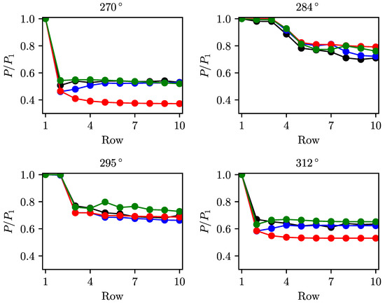
Figure 4.
Wind farm power production of Columns 2–4 (counting from the south) at various wind angles from large-eddy simulations (LES) (black), the Jensen model (red), the coupled wake boundary layer (CWBL) (blue), and the present model (green). LES data were digitally extracted from [24].
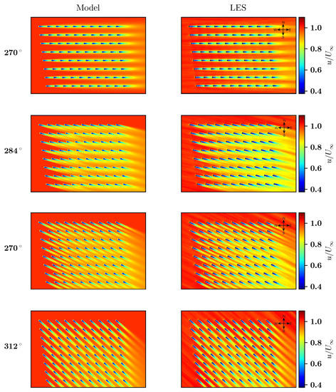
Figure 5.
Velocity field of Horns Rev wind farm at various wind angles. Results compare the current model (left) to time-averaged LES velocity fields (right). LES fields reproduced from [44], which is licensed under the Creative Commons Attribution CC-BY 3.0 license.
4. A Control-Oriented Dynamic Model
Models for active and closed-loop control applications need to account for the effect of wind turbine control actions on other turbines. In Section 4.1, we apply the dynamic model described in Section 2 to an extreme example of such a problem, a wind farm at start-up. We simulate the model with both linear and non-linear advection and compare the results to ensemble-averaged LES. In Section 4.2, we provide measurement-based state and parameter estimation algorithms. The first provides a filter to obtain estimates of the time-varying, spanwise inhomogenous inflow velocities. We then apply an ensemble Kalman filter (EnKF) to correct for modeling errors, such as the linear advection assumption and additional turbulence effects, which are not fully accounted for in the model. Finally, the dynamic model with state and parameter estimation is compared to LES data.
4.1. Dynamic Thrust Modulation
In this section, we test the model’s capability to capture the dynamics of wake advection in response to dynamic changes in a wind turbine’s thrust control actions. Specifically, we examine the power output trajectory in each row of the farm using the LES results from a wind farm at start-up [8]. Both the LES and the model are applied to a wind farm composed of 14 rows of 10 turbines with streamwise and spanwise spacings of and , respectively. Each turbine has a rotor diameter of m, hub height of m, and operating thrust coefficient of . The incoming atmospheric boundary layer flow has a friction velocity of m/s and roughness height m. The inflow velocity is therefore set as , where is the von Karman constant. The wind farm start-up is modeled as a step change in the local thrust coefficient from to . The model is simulated using the linear and nonlinear advection velocities discussed in Section 2. The wake expansion coefficients are determined using the top-down coupling approach discussed in Section 3, with .
The dynamic change in power for the first four rows, where the total power for the entire row is plotted, is shown in Figure 6. An ensemble of 20 LES realizations is averaged to reduce the effect of turbulent fluctuations and focus on the dynamic effects during start-up. The results demonstrate that the model is able to accurately predict the power levels of the wind farm using only the layout of the farm, the inflow friction velocity and the roughness height. The linear model results are similar to those seen in [8]. In this case, however, the wake expansion coefficients are not set by fitting the steady-state simulation data because the extended framework described in Section 3 provides a means of calculating the wake expansion coefficients. As expected, the nonlinear advection model provides a better prediction of the dynamics, particularly where the first wake hit the downstream turbine at min.
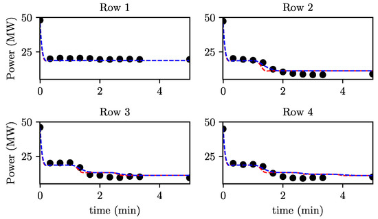
Figure 6.
Power production of a wind farm at start-up comparing LES (symbols), the model with linear advection (red), and the model with nonlinear advection (blue). Only the first four rows of the farm are shown.
4.2. State and Parameter Estimation
In this section, we use the power measurements that are readily available in physical wind farms as feedback for a state and parameter estimation. This type of estimation scheme would be used in a control application in order to correct for modeling errors and unmodeled effects such as turbulent fluctuations that are clearly visible in the spectrum of wind turbine power production [45]. To demonstrate the effectiveness of this approach, we introduce a known error into the model by using the linear advection model.
We first present an empirical model of the local inlet velocity that accounts for the known large-scale streaks and rolls [46] that generate spanwise variability in the inflow velocity. The model is based on estimates of the freestream velocity from the power measurements collected from unwaked turbines in the farm; i.e., those turbines whose power output is not affected by wakes of upstream turbines. The velocity magnitudes collected from these unwaked turbines are then time filtered using a linear temporal relaxation towards the instantaneous values, according to:
The set denotes the set of unwaked turbines in the farm, and min is the relaxation time constant by which the measurements are effectively filtered.
These filtered inflow velocities are used in two ways. First, the linear advection velocity model is used with the advection velocity in (1) set to the mean of the filtered inflow velocities , where is the number of unwaked turbines. While this approach is known to be less accurate than using the nonlinear advection model, it introduces a known error that enables us to demonstrate the effectiveness of this approach. In particular, errors due to this assumption are mitigated through the updated measurements of the power at each turbine and at each time-step. A linear model may also be preferred to simplify computations and analysis. Second, a spanwise profile of the incoming velocity is generated by linearly interpolating between the freestream velocity points found above. This spanwise profile is used to find the velocity field for (5).
An EnKF is used to reduce the error in the velocity deficits (the states of the model) and the wake expansion coefficients (the parameters of the model) based on power measurements at each turbine. In particular, we extend the approach of Shapiro et al. [37] to incorporate the modified dynamic model presented in this paper. This extension allows the estimation method to be applied to arbitrary turbine configurations and includes spanwise variations in inflow velocities. We recall that the previous approach of Shapiro et al. [37] was limited to regular wind farm configurations in which all rows were averaged and the farm could be treated as a single column of representative turbines.
The EnKF assumes that the resulting modeled wind farm system is governed by the discrete update equations:
where and are temporal and spatial discretizations of the wake model, is the vector of the model states, is a vector of the local thrust coefficients at each turbine, and the function maps the states to the measured quantities (the power at each turbine). Measurement and modeling errors are represented by the zero-mean white noise processes and , respectively. The assumed root-mean-square (RMS) of the measurement, state, and parameter noises must be prescribed. In the examples shown, they are specified as m/s, , and kW.
An ensemble of 256 wake model implementations, governed by (38) and (39), is used to estimate the error covariance of the wake model compared to measurements. The state and parameter estimates are computed in two steps. First, the wake model is used to perform an intermediate forecast of the wake model states. Then, power measurements are used in conjunction with the ensemble estimates in the measurement analysis step to produce states and parameter estimates. Further details of this method can be found in [37].
The estimation algorithm is tested using an LES of a 38-turbine wind farm composed of four staggered rows of six turbines followed by 14 irregularly-arranged turbines at the back of the farm, as shown in Figure 7. This arrangement allows us to demonstrate the utility of this approach on wind farms with both regularly- and irregularly-spaced turbines. The simulations are performed using the pseudo-spectral code LESGO [47], which is open source and publicly available at https://lesgo.me.jhu.edu/, using the concurrent precursor inflow method [48], the Lagrangian-averaged scale-dependent subgrid scale model [49], and actuator disk wind turbine models [25,39]. The domain extends km in the streamwise, spanwise, and vertical directions with grid points in these directions, respectively. The friction velocity is set to be m/s, and the surface roughness height is specified as m. The turbines have a rotor diameter of m, a hub height of m, and a local thrust coefficient of .
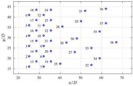
Figure 7.
Locations of the 38 turbines in the wind farm simulated in LES.
The measured and estimated power production for six turbines, which are representative of the farm, are shown in Figure 8. The estimated power production show very good agreement with the measurements. The RMS error has a value of kW, which corresponds to a percent error of . The modeled velocity field at min is compared to a time-averaged LES velocity field averaged between min and min in Figure 9. As demonstrated by this plot, the state-estimated dynamic wake model generates realistic velocity fields at a computational cost that is significantly lower than higher fidelity approaches like LES or RANS. Specifically, for this simulation comprised of an ensemble of 256 perturbed wake models, the ensemble calculations are spread over 32 processors, which means that each processor handles eight of the ensemble members. The average time to advance these models is s for a simulation time step of s, which means that these calculations can be computed in real time based on typical wind farm control loops.
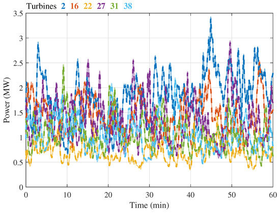
Figure 8.
Measured (——)and estimated power production (– – –) for the 38-turbine wind farm. The turbine locations are shown in Figure 7.
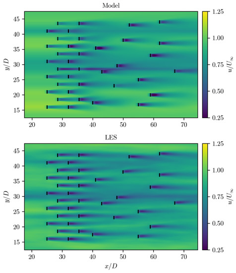
Figure 9.
Comparison of state-estimated dynamic wake model velocity fields at min and LES averaged between min and min.
5. Conclusions
We introduced a continuous-time dynamic wake model and its steady-state counterpart, which provided a unifying framework for studying wind farm design and control problems. Our previously-proposed dynamic model was extended by deriving the linear wake expansion scaling from self-similarity, showing rigorously that and developing a realistic wake profile function that transitioned from a top-hat profile to a Gaussian. For steady-state design problems, the developing top-down model was coupled to the wake model to specify the wake expansion coefficient properly and closely match LES data. The dynamic model was shown to reproduce the behavior of a wind farm at start-up. State and parameter estimation was used to incorporate unmodelled turbulence effects, as well as variations in spanwise inflow velocity and streamwise advection velocities. These extensions lay the groundwork for improving wind farm design and control optimization by providing physics-based estimates of the wake expansion rate, more accurately predicting the wind farm advection time, and generating more realistic wind farm velocity fields through realistic wake profiles and state estimation.
Author Contributions
C.R.S. formulated the problem, analyzed results and wrote the first draft of the paper. G.M.S. formulated the problem, performed the simulations and analyzed results in Section 4.2. C.M. and D.F.G. helped formulate the problem, interpret the results and contributed to writing the paper.
Funding
This material is based on work supported by the National Science Foundation under Grant No. CMMI 1635430 and the National Science Foundation Graduate Research Fellowship under Grant No. DGE 1746891. Computations were made possible by Maryland Advanced Research Computing Center (MARCC).
Acknowledgments
The authors thank R.J.A.M. Stevens and J. Meyers for useful conversations at the initial stages of this research and P. Bauweraerts for the start-up LES data.
Conflicts of Interest
The authors declare no conflicts of interest.
References
- Lackner, M.A.; Elkinton, C.N. An Analytical Framework for Offshore Wind Farm Layout Optimization. Wind Eng. 2007, 31, 17–31. [Google Scholar] [CrossRef]
- Chowdhury, S.; Zhang, J.; Messac, A.; Castillo, L. Unrestricted wind farm layout optimization (UWFLO): Investigating key factors influencing the maximum power generation. Renew. Energy 2012, 38, 16–30. [Google Scholar] [CrossRef]
- Bokharaie, V.S.; Bauweraerts, P.; Meyers, J. Wind-farm layout optimisation using a hybrid Jensen–LES approach. Wind Energy Sci. 2016, 1, 311–325. [Google Scholar] [CrossRef]
- Adcock, C.; King, R.N. Data-driven wind farm optimization incorporating effects of turbulence intensity. In Proceedings of the 2018 Annual American Control Conference (ACC), Milwaukee, WI, USA, 27–29 June 2018; pp. 701–706. [Google Scholar] [CrossRef]
- Fleming, P.A.; Gebraad, P.M.; Lee, S.; van Wingerden, J.W.; Johnson, K.; Churchfield, M.; Michalakes, J.; Spalart, P.; Moriarty, P. Evaluating techniques for redirecting turbine wakes using SOWFA. Renew. Energy 2014, 70, 211–218. [Google Scholar] [CrossRef]
- Annoni, J.; Scholbrock, A.; Churchfield, M.; Fleming, P. Evaluating tilt for wind plants. In Proceedings of the 2017 Annual American Control Conference (ACC), Seattle, WA, USA, 24–26 May 2017; pp. 717–722. [Google Scholar] [CrossRef]
- De Rijcke, S.; Driesen, J.; Meyers, J. Power smoothing in large wind farms using optimal control of rotating kinetic energy reserves. Wind Energy 2015, 18, 1777–1791. [Google Scholar] [CrossRef]
- Shapiro, C.R.; Bauweraerts, P.; Meyers, J.; Meneveau, C.; Gayme, D.F. Model-based receding horizon control of wind farms for secondary frequency regulation. Wind Energy 2017, 20, 1261–1275. [Google Scholar] [CrossRef]
- Bay, C.J.; Annoni, J.; Taylor, T.; Pao, L.; Johnson, K. Active power control for wind farms using distributed model predictive control and nearest neighbor communication. In Proceedings of the 2018 Annual American Control Conference (ACC), Milwaukee, WI, USA, 27–29 June 2018; pp. 701–706. [Google Scholar] [CrossRef]
- Boersma, S.; Doekemeijer, B.; Siniscalchi-Minna, S.; van Wingerden, J. A constrained wind farm controller providing secondary frequency regulation: An LES study. Renew. Energy 2019, 134, 639–652. [Google Scholar] [CrossRef]
- Vali, M.; Petrović, V.; Boersma, S.; van Wingerden, J.W.; Pao, L.Y.; Kühn, M. Adjoint-based model predictive control for optimal energy extraction in waked wind farms. Control Eng. Pract. 2019, 84, 48–62. [Google Scholar] [CrossRef]
- Goit, J.P.; Meyers, J. Optimal control of energy extraction in wind-farm boundary layers. J. Fluid Mech. 2015, 768, 5–50. [Google Scholar] [CrossRef]
- Munters, W.; Meyers, J. Dynamic strategies for yaw and induction control of wind farms based on large-eddy simulation and optimization. Energies 2018, 11, 177. [Google Scholar] [CrossRef]
- Jensen, N.O. A Note on Wind Generator Interaction; Technical Report Risø-M-2411; Risø National Laboratory: Roskilde, Denmark, 1983. [Google Scholar]
- Katic, I.; Højstrup, J.; Jensen, N.O. A simple model for cluster efficiency. In Proceedings of the European Wind Energy Association Conference and Exhibition, Rome, Italy, 7–9 October 1986; pp. 407–410. [Google Scholar]
- Bastankhah, M.; Porté-Agel, F. A new analytical model for wind-turbine wakes. Renew. Energy 2014, 70, 116–123. [Google Scholar] [CrossRef]
- Ge, M.; Wu, Y.; Liu, Y.; Yang, X.I. A two-dimensional Jensen model with a Gaussian-shaped velocity deficit. Renew. Energy 2019, 141, 46–56. [Google Scholar] [CrossRef]
- Gebraad, P.M.O.; van Wingerden, J.W. A Control-Oriented Dynamic Model for Wakes in Wind Plants. J. Phys. Conf. Ser. 2014, 524, 012186. [Google Scholar] [CrossRef]
- Frandsen, S.; Barthelmie, R.; Pryor, S.; Rathmann, O.; Larsen, S.; Højstrup, J.; Thøgersen, M. Analytical modelling of wind speed deficit in large offshore wind farms. Wind Energy 2006, 9, 39–53. [Google Scholar] [CrossRef]
- Niayifar, A.; Porté-Agel, F. A new analytical model for wind farm power prediction. J. Phys. Conf. Ser. 2015, 625, 012039. [Google Scholar] [CrossRef]
- Niayifar, A.; Porté-Agel, F. Analytical Modeling of Wind Farms: A New Approach for Power Prediction. Energies 2016, 9, 741. [Google Scholar] [CrossRef]
- Peña, A.; Rathmann, O. Atmospheric stability-dependent infinite wind-farm models and the wake-decay coefficient. Wind Energy 2013, 17, 1269–1285. [Google Scholar] [CrossRef]
- Stevens, R.J.A.M.; Gayme, D.F.; Meneveau, C. Coupled wake boundary layer model of wind-farms. J. Renew. Sustain. Energy 2015, 7, 023115. [Google Scholar] [CrossRef]
- Stevens, R.J.A.M.; Gayme, D.F.; Meneveau, C. Generalized coupled wake boundary layer model: Applications and comparisons with field and LES data for two wind farms. Wind Energy 2016, 19, 2023–2040. [Google Scholar] [CrossRef]
- Calaf, M.; Meneveau, C.; Meyers, J. Large eddy simulation study of fully developed wind-turbine array boundary layers. Phys. Fluids 2010, 22, 015110. [Google Scholar] [CrossRef]
- Meneveau, C. The top-down model of wind farm boundary layers and its applications. J. Turbul. 2012, 13, N7. [Google Scholar] [CrossRef]
- Martínez-Tossas, L.A.; Annoni, J.; Fleming, P.A.; Churchfield, M.J. The aerodynamics of the curled wake: A simplified model in view of flow control. Wind Energy Sci. 2019, 4, 127–138. [Google Scholar] [CrossRef]
- Bastankhah, M.; Porté-Agel, F. Experimental and theoretical study of wind turbine wakes in yawed conditions. J. Fluid Mech. 2016, 806, 506–541. [Google Scholar] [CrossRef]
- Jiménez, Á.; Crespo, A.; Migoya, E. Application of a LES technique to characterize the wake deflection of a wind turbine in yaw. Wind Energy 2010, 13, 559–572. [Google Scholar] [CrossRef]
- Larsen, G.C.; Madsen, H.A.; Thomsen, K.; Larsen, T.J. Wake meandering: a pragmatic approach. Wind Energy 2008, 11, 377–395. [Google Scholar] [CrossRef]
- Gebraad, P.M.O.; Teeuwisse, F.W.; van Wingerden, J.W.; Fleming, P.A.; Ruben, S.D.; Marden, J.R.; Pao, L.Y. Wind plant power optimization through yaw control using a parametric model for wake effects-a CFD simulation study. Wind Energy 2016, 19, 95–114. [Google Scholar] [CrossRef]
- Shapiro, C.R.; Gayme, D.F.; Meneveau, C. Modelling yawed wind turbine wakes: a lifting line approach. J. Fluid Mech. 2018, 841. [Google Scholar] [CrossRef]
- Boersma, S.; Doekemeijer, B.; Vali, M.; Meyers, J.; van Wingerden, J.W. A control-oriented dynamic wind farm model: WFSim. Wind Energy Sci. 2018, 3, 75–95. [Google Scholar] [CrossRef]
- Bauweraerts, P.; Meyers, J. On the Feasibility of Using Large-Eddy Simulations for Real-Time Turbulent-Flow Forecasting in the Atmospheric Boundary Layer. Bound.-Layer Meteorol. 2019, 171, 213–235. [Google Scholar] [CrossRef]
- Frandsen, S. On the wind speed reduction in the center of large clusters of wind turbines. J. Wind Eng. Ind. Aerodyn. 1992, 39, 251–265. [Google Scholar] [CrossRef]
- Doekemeijer, B.M.; Boersma, S.; Pao, L.Y.; van Wingerden, J.W. Ensemble Kalman filtering for wind field estimation in wind farms. In Proceedings of the 2017 Annual American Control Conference (ACC), Seattle, WA, USA, 24–26 May 2017; pp. 19–24. [Google Scholar] [CrossRef]
- Shapiro, C.R.; Meyers, J.; Meneveau, C.; Gayme, D.F. Dynamic wake modeling and state estimation for improved model-based receding horizon control of wind farms. In Proceedings of the 2017 Annual American Control Conference (ACC), Seattle, WA, USA, 24–26 May 2017; pp. 709–716. [Google Scholar] [CrossRef]
- Burton, T.; Jenkins, N.; Sharpe, D.; Bossanyi, E. Wind Energy Handbook; John Wiley & Sons: Chichester, West Sussex, UK, 2011. [Google Scholar]
- Meyers, J.; Meneveau, C. Large Eddy Simulations of Large Wind-Turbine Arrays in the Atmospheric Boundary Layer. In Proceedings of the 48th AIAA Aerospace Sciences Meeting, Orlando, FL, USA, 4–7 January 2010; p. 827. [Google Scholar] [CrossRef]
- Tennekes, H.; Lumley, J.L. A First Course in Turbulence; MIT: Cambridge, MA, USA, 1972. [Google Scholar]
- Gradshteyn, I.; Ryzhik, I. Table of Integrals, Series, and Products: Corrected and Enlarged Edition; Academic Press: New York, NY, USA, 1980. [Google Scholar]
- Stevens, R.J.A.M.; Gayme, D.; Meneveau, C. Using the coupled wake boundary layer model to evaluate the effect of turbulence intensity on wind farm performance. J. Phys. Conf. Ser. 2015, 625, 012004. [Google Scholar] [CrossRef]
- Crespo, A.; Frandsen, S.; Gómez-Elvira, R.; Larsen, S.E.; Petersen, E.L.; Hjuler Jensen, P.; Rave, K.; Helm, P.; Ehmann, H. Modelization of a large wind farm, considering the modification of the atmospheric boundary layer. In Proceedings of the European Wind Energy Conference, Nice, France, 1–5 March 1999. [Google Scholar]
- Porté-Agel, F.; Wu, Y.T.; Chen, C.H. A Numerical Study of the Effects of Wind Direction on Turbine Wakes and Power Losses in a Large Wind Farm. Energies 2013, 6, 5297–5313. [Google Scholar] [CrossRef]
- Stevens, R.J.A.M.; Meneveau, C. Temporal structure of aggregate power fluctuations in large-eddy simulations of extended wind-farms. J. Renew. Sustain. Energy 2014, 6, 043102. [Google Scholar] [CrossRef]
- Kline, S.J.; Reynolds, W.C.; Schraub, F.A.; Runstadler, P.W. The structure of turbulent boundary layers. J. Fluid Mech. 1967, 30, 741. [Google Scholar] [CrossRef]
- Stevens, R.J.A.M.; Martínez, L.A.; Meneveau, C. Comparison of wind farm large eddy simulations using actuator disk and actuator line models with wind tunnel experiments. Renew. Energy 2018, 116, 470–478. [Google Scholar] [CrossRef]
- Stevens, R.J.; Graham, J.; Meneveau, C. A concurrent precursor inflow method for Large Eddy Simulations and applications to finite length wind farms. Renew. Energy 2014, 68, 46–50. [Google Scholar] [CrossRef]
- Bou-Zeid, E.; Meneveau, C.; Parlange, M. A scale-dependent Lagrangian dynamic model for large eddy simulation of complex turbulent flows. Phys. Fluids 2005, 17, 025105. [Google Scholar] [CrossRef]
© 2019 by the authors. Licensee MDPI, Basel, Switzerland. This article is an open access article distributed under the terms and conditions of the Creative Commons Attribution (CC BY) license (http://creativecommons.org/licenses/by/4.0/).