Abstract
Temperature measuring point is the key to room environment control. Temperature measuring points and climate changes are directly related to the room control effect. It is of great theoretical and practical significance to study the temperature measuring points and control strategy based on climate compensation. In this study, first, the climate compensation concept in a heating system was introduced into a variable air volume (VAV) air-conditioning system. The heating load was modeled as a function of supply air temperature by analyzing the heat exchange. Based on each control link of subsystems, a climate compensation scheme is proposed to determine the optimal set-point of the supply air temperature. At the same time, a layout of multiple temperature measuring points of an air-conditioned room was studied. Furthermore, the optimal indoor temperature measuring point was determined using an adaptive weighted fusion method. Finally, simulation results show that the proposed method has better control effects on indoor temperature adjustment compared with the traditional method. The optimal supply air temperature in summer and winter was determined according to the proposed climate compensation scheme, and the supply air temperature was controlled using an improved single-neuron adaptive control strategy. Experimental results show that the maximum energy saving can reach up to 35.5% in winter and 6.1% in summer.
1. Introduction
The variable air volume (VAV) air-conditioning control system can be individually controlled according to different needs of different air-conditioned areas. Moreover, by changing the volume of air supplied to each room, it is possible to satisfy the indoor load change to achieve energy saving.
The heat consumption of buildings changes with the change of outdoor climate and temperature, and the indoor load will also change as follow. If the supply water temperature remains unchanged, it will often cause the phenomenon of indoor supercooling or overheating, which will result in serious wastes of energy. In an air-conditioning system, the existing climate compensation and energy-saving control strategy refers to the central air conditioning to adjust the chilled water supply or return water temperature of the chiller according to the external climate changes. In a heating system, a climate compensator can be used to solve the problem of imbalance between the heat source and terminal heating load (users’ needs) theoretically based on the outdoor temperature to adjust the heat output to control the supply water temperature of the system. Furthermore, the supply water temperature can be controlled within the allowable range of theoretical calculation. A climate compensator is widely used in engineering processes at present [1,2,3,4]. The relationship between supply and return water temperature and the indoor and outdoor temperature was determined by theoretical calculation and can be changed according to the actual situation. In practical engineering, the climate compensation reform system in a boiler room is added to a building divided period, and divided temperature control can reduce the heating energy consumption by 20% [3]. The existing climate compensation energy-saving control technology of central air-conditioning system controls the water system to achieve the climate compensation of temperature of chilled water supply and also achieve the energy saving of water system without considering the effect on wind system [5,6]. Furthermore, the fresh air volumes also significantly affect the whole energy consumption of air-conditioning system. Engdahl and Johansson established a model to study the energy-saving potential of VAV air-conditioning systems with constant and variable values, respectively [7]. The model results showed that compared to constant supply air temperature, variable supply air temperature has 8–27% energy-saving potential [8]. If a climate compensation in a heating system is applied to the wind system of VAV air-conditioning system, the supply air temperature can be changed in real time according to the outdoor climate. It also has a certain energy-saving effect.
Supply air temperature is one of the main parameters of a VAV air-conditioning system, which is constant in conventional control. However, changing the supply air temperature in real time has a more effective control effect [7]. Currently, air-conditioning systems are more commonly used for indoor temperature control based on a single indoor temperature sensor detection. However, most indoor sensors are unreasonably arranged. This affects the detection of indoor temperature and thus affects the system control effect, thereby causing uneven indoor temperature distribution. If the indoor optimal temperature measuring points can be found and the indoor temperature is controlled according to the optimal measuring points, the system control effect, indoor temperature unevenness, and indoor temperature comfort can be effectively improved.
In [9], the supply air temperature was optimized through the temperature difference between the two air nodes in an air-conditioned room, changing the room temperature and comfort of indoor personnel. In [10], a fan energy consumption model and a pump energy consumption model were established. With the minimum energy consumption of an air-conditioning unit as the target, the optimal supply air temperature of air-conditioning unit under different working conditions was solved using the operation performance of cooling coil, and the air-conditioning operating parameters were optimized. In [11], a temperature and humidity control system based on multi-sensor data fusion was performed on temperature and humidity using an adaptive weighted average algorithm. Based on the combined temperature and humidity data, the control strategy was determined, and the greenhouse environmental parameters were adjusted to improve the accuracy and reliability of the system. Kojima and Kazuyuki [12] predicted human thermal comfort and sensation using a network of 21 temperature sensors placed in an indoor environment in an office air-conditioning system. In [13], a supply air control strategy based on a multi-sensor scheme was proposed for VAV air-conditioning systems. Simulation results show that the indoor air temperature field and velocity field distribution can be optimized based on multi-sensor control. Furthermore, the thermal comfort environment of human body can be better improved, and the system energy consumption can be reduced by optimization. These studies show that the indoor temperature field characteristics affect the thermal comfort of human body, and the indoor temperature sensor position affects the indoor temperature field characteristics. The actual VAV air-conditioning system mainly controls the system by collecting the detection values of each sensor.
Motivated by the aforementioned issues, we firstly study the indoor temperature sensor arrangement to determine the optimal measuring points of indoor temperature in air-conditioned rooms. Then, the value of indoor temperature fusion is used to obtain the optimal indoor temperature measurement point. Finally, the controlled air damper at the terminal of VAV system and the room object are identified and simulated. On this basis, terminal control is evaluated. This study is based on the experimental platform of VAV air-conditioning system of Institute of Intelligent Buildings in Xi’an University of Architecture and Technology. The optimal measuring point and terminal control strategy of indoor temperature in air-conditioned rooms were evaluated.
2. Climate Compensator
At present, central air-conditioning systems have two types of climate compensation energy-saving technology, i.e., (i) by adjusting the operating parameters of a chiller, the temperature of chilled water in an air-conditioning system can be adjusted according to the external climate to achieve energy saving [6]; and (ii) by adjusting the control valve in the water supply line and using a constant temperature controller, the water flow can be adjusted to control the difference in supply and return water temperature [6]. The two methods can achieve the energy saving of an air-conditioning water system by evaluating the effect of external climate change on it.
The energy consumption of an air-conditioning system is directly related to building envelope, outdoor climate parameters, and indoor heat dispersion or humidity dispersion. When the pipe network capacity of an air-conditioning system, building type, construction area, and other factors are determined, under the premise of satisfying the room temperature demand, the main factors influencing the air-conditioning load are outdoor temperature and fresh air load. Air-conditioning load is a dynamic parameter and cannot be measured directly; it is difficult to control the air-conditioning load directly through load monitoring. Therefore, it is necessary to represent the load as a measurable parameter, reflecting the output change in a heat source or cooling source in a timely manner. Heat exchange between the water system and air system is carried out in the heat exchanger of air handling unit (AHU) of VAV air-conditioning system. The heat exchanged by the heat exchanger can directly reflect the output of heat source; the opening of the chilled water valve affects the supply air temperature directly. Therefore, such a parameter can be determined by the heat exchange analysis of heat exchanger.
2.1. Analysis of Cooling Load in Summer Condition
The cooling load of an air-conditioned area in summer is mainly caused by the difference in indoor and outdoor temperatures and the heat of solar radiation entering the room through the building envelope. In the working process of an air-conditioning system, the heat produced by the fan and pump and the heat produced by the wind duct, water pipe, and other mechanical changes are also important parts that cannot be ignored [14]. The outdoor temperature and enthalpy are higher than the indoor circumstance, and the air-conditioning system needs more energy to deal with the fresh air than the return air. Therefore, the main effects of air-conditioning energy consumption of buildings in summer are the heat consumption of building envelope structure, fresh air load, and the cooling load produced by other forms of heat in the air-conditioning system. It is assumed that the heat gain of an air-conditioning system in the summer condition does not include the heat delivered by radiation.
The changes in cooling load in an air-conditioning system are mainly due to the indoor cooling load and fresh air-cooling load. The indoor cooling load is caused by the change in indoor temperature and outdoor temperature . The fresh air-cooling load is mainly caused by the change in outdoor temperature . Therefore, the air-conditioning system cooling load can be modeled by the relationship between indoor temperature and outdoor temperature :
In Equation (1), the relationship between supply air temperature and outdoor temperature can be expressed as:
where is supply air temperature. Therefore, the supply air temperature in a VAV air-conditioning system can satisfy the two requirements of above parameters. When the outlet water temperature of the chiller is constant and the flow of water system is variable, the supply air temperature not only reflects the chiller output size, but also can be identified in the corresponding outdoor temperature according to dissatisfy users’ demands. Furthermore, the supply air temperature can be used as a control parameter to adjust the cold source output.
2.2. Analysis of Heating Load in Winter Condition
The heating load of buildings in winter can be determined according to the heat loss and heat gain of buildings. In civil buildings, an air-conditioned room should maintain a positive pressure, and the cold air consumption occurring through the gap of door and window into a room can be ignored. Therefore, the main factors affecting the energy consumption of air-conditioning in buildings are envelope consumption, the load generated by an indoor heat source, and the handling load of fresh air. The outdoor temperature is lower than the indoor temperature in winter, and indoor humidity is low. The air-conditioning system has more energy consumption when dealing with fresh air [14]. The relationship between the heating load in room, current indoor temperature, and current outdoor temperature can be expressed as follows:
Using Equation (3), the relationship between supply air temperature and outdoor temperature can be expressed as follows:
Therefore, the supply air temperature satisfied two conditions of above parameters in the VAV air-conditioning system, i.e., in the case of constant outlet water temperature of heat source and variable water system flow, the supply air temperature not only reflects the size of heat source, but also can be determined dissatisfy users’ demands in the corresponding outdoor temperature. It can be used as a control parameter to adjust the heat output.
3. Control System
This study is based on the experimental system of the VAV laboratory of Xi’an University of Architecture and Technology. The structure of the system is mainly divided into three layers: Information layer, control layer, and original layer. The information layer includes data storage system of SQL-Sever and LabVIEW-based monitoring system; the control layer is PLC field device control; the original layer is a plurality of electrical quantity transducers, frequency changer, and other sensors and actuators connected by RS485 bus.
The VAV air-conditioning terminal system includes pressure-independent VAV BOX of Royal Service, temperature control panel of Belimo, control actuator, temperature and humidity sensors, and other equipment. The VAVBOX is the VAV terminal device. It can track the change of indoor load by changing the opening of air valve, so that the temperature and humidity of air-conditioned room are within the comfort range of human body.
The terminal device is a single-duct type terminal, and the model is RSV-TU-1-I-06-L-(D-SA). The VAV control actuator is LMV-D2-MFT-RM from Belimo. The controller and the actuator are integrated. The T24-b from Belimo is selected as temperature controller. The valve position feedback device P500A reflects the current position of VAV damper through the resistance value. The local control of VAV system is carried out by combining all parts as shown in Figure 1.
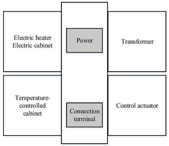
Figure 1.
Terminal diagram of VAV BOX controller.
The specific parameters are as follows: The minimum and maximum air volume are 140 CMH and 500 CMH respectively. The discharge coefficient is 0.8, and the reheating capacity is 2.5 kW. It can be divided into box body and control part. The electric cabinet is the main control part of the total terminal device; it involves the air volume controller and controlled object. The composition structure of the controlled object is shown in Figure 2.
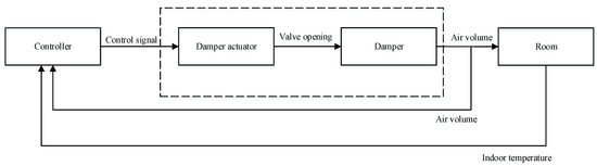
Figure 2.
Composition structure of the controlled object.
The climate compensation strategy for VAV air conditioning studied in this paper involves the optimization of steady-state set-points. In the experiments, sufficient heat (cold) is required, and the subsystems need to operate stably under a closed-loop control. Therefore, it is necessary to control the water temperature of heat (cold) source, water differential pressure of secondary pump water systems, supply air temperature, and terminal room temperature. Among them, taking the smallest quantity of fresh air volume (opening of fresh air valve at 10%), the cooling water system operated in constant flow in summer condition and the set-point are based on previous studies. The water system adopts a constant flow operation mode in winter condition, and the room temperature can be controlled using the controller of experimental system, which can be controlled using the system’s own controller.
A VAV air-conditioning system operating in the summer condition mainly includes a cold source outlet water temperature control, constant differential pressure control of secondary pump, supply air temperature control, and fan constant static pressure control; in the winter condition, the VAV air-conditioning system includes a heat source outlet water temperature control, supply air temperature control, and fan constant static pressure control.
The sensor parameters of the experimental system in this study are as shown in Table 1.

Table 1.
Sensor parameters.
3.1. Cold and Heat Source Control
The nominal cooling capacity of cold source is 18 kW; the compressor cooling capacity is 3.9 kW; the cold inlet/outlet temperature is 12 °C/7 °C; the heat source side inlet/outlet water temperature is 30 °C/35 °C. Because of environmental constraints, the heat pump unit was only used for summer cooling in this study and considered as a chiller.
The stable operation of the chiller in the air-conditioning system guarantees enough cooling capacity. When a variable flow control is used in water system, it must maintain a constant outlet temperature of chilled water. At the same time, the temperature should not be below the safety threshold of the chiller. The laboratory room has no continuous load; after working for a period of time, the temperature of chilled water drops to the safety limit and stops. Therefore, a heater was used in the experiment to simulate the load of terminal.
When the temperature of outlet chilled water is lower than the lower limit A, the heater starts; when the temperature is higher than the upper limit B, the heater closes. To maintain the temperature of outlet chilled water in a small range, it can be approximately regarded as a stable control. The upper and lower limits of control are determined by the expected control of temperature of outlet chilled water. CH1 (chiller) outlet chilled water temperature was used to control the heater in the experiment. The lower control limit was set as 7.5 °C; the upper control limit was set as 8.5 °C. Then, the outlet chilled water temperature of the chiller was maintained at 8 °C through program control. The experimental data show that the outlet water temperature is stable in the set range, and the effect of cold source outlet water temperature control is ideal.
An electric heater equipped with two electric heating rods was used as the heat source, and the power of single rod was 15 kW. The heat source water temperature control had “on-off” control. As shown in Figure 3, the heat source outlet water temperature was set to 35 °C. The heater was started and stopped by the temperature set-point and the upper and lower limits. The outlet water temperature was maintained at 35 °C (±1 °C), satisfying the requirements. The temperature sensor was placed at a distance from the heater and the system had inertia. Therefore, the water temperature showed a certain fluctuation and hysteresis (the heaters are turned on and off; the temperature fluctuation is about 1 °C.).
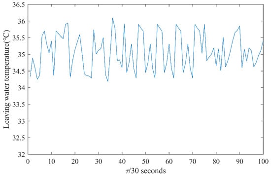
Figure 3.
Effects of heat source outlet water temperature control.
3.2. Incremental Constant Differential Pressure Control of Secondary Pump
Figure 4 shows the structure of secondary pump constant differential pressure. The differential pressure sensor detects the actual supply and return water pipe pressure, and the controller controls the inverter according to the difference between the set-point and test value to change the pump speed, so that the differential pressure between the supply and return water is recovered to the set-point. The detection position of differential pressure transducer is located at the ends of both supply and return water main pipe.
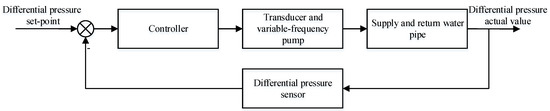
Figure 4.
Structure of secondary pump constant differential pressure control.
The valve opening degree changes during the supply air temperature adjustment, causing a change in the pipe differential pressure. Therefore, the water pump is regulated by frequency conversion, and the differential pressure of pipeline is returned to the desired value using a controller. In this control loop, an actuator is required to control the amount of incremental. The frequency of secondary pump is controlled by incremental PID (proportional-integral-derivative) controller. Its control algorithm can be expressed as follows:
where is the increment, is proportionality coefficient, is integral time constant, and is differentiating time constant. Through the experimental debugging and past experience, the differential pressure set-point was selected as 0.10 MPa. The output amplitude of controller is 20–50 Hz, and the PID parameters are set as = 20.30, = 19.7974, and = 37.1178. Experimental results show that after a period of time, the pressure difference of the secondary pump can be stabilized near the set-point.
3.3. PI Control of Constant Static Pressure
A VAV air-conditioning system can adjust the fan speed according to the change in terminal load, so that the volume of supply air satisfies the actual demand. There are three types of control methods: Constant static pressure control, variable static pressure control, and total air volume control. In this study, the static pressure control method was used to monitor the static pressure of the most unfavorable loop of supply air pipe in real time. A frequency converter was used in the static pressure controller to change the fan speed to maintain the static pressure. Figure 5 shows the control structure. The static pressure set-point is 220 Pa; the frequency range of supply fan in the experiment is 20–45 Hz. The frequency of fan was controlled using a PI controller, so that the static pressure was maintained within the allowable range. The optimal parameters were obtained using the simplex optimization method; specific parameters are = 0.065, = 0.25 min. As shown in Figure 6, it is the actual static pressure of duct, and the control effect satisfies the experimental needs.
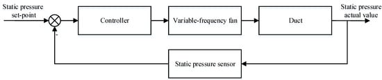
Figure 5.
Structure of fan static pressure control.
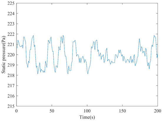
Figure 6.
Static pressure control effect of AHU2.
3.4. Improved Single Neuron PID Control of Supply Air Temperature
Neural networks have obvious advantages in the control of complex systems. Research on neural network control and identification have become the mainstream of intelligent control research. The single-neuron adaptive PID control algorithm is superior to the traditional PID control algorithm in general, which is beneficial to the improvement of control system quality, less affected by the environment, and has strong control robustness. It is a promising controller.
Figure 7 shows the structure of supply air temperature control. The sensor detects the actual supply air temperature and transmits it to the controller. The deviation was obtained by comparing with the set-point of supply air temperature. Then, the controller adjusts the opening value of chilled water valve according to the deviation, changes the flow rate of chilled water, and controls the temperature of supply air. The opening value of chilled water valve has a nonlinear relationship with the water flow. When the opening value is less than 2% or greater than 45%, the flow of chilled water remains unchanged, equivalent to the minimum or maximum values, respectively. In this study, by combining with the valve opening flow characteristics, the opening of chilled water valve was set at 2–35%.
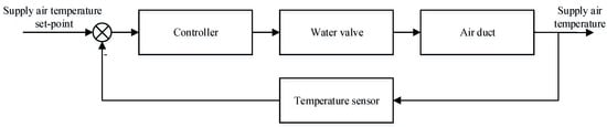
Figure 7.
Structure of supply air temperature control.
3.4.1. Improved Single Neuron PID Control in Summer Condition
Because of a large hysteresis of supply air temperature control system, an improved single neuron control algorithm was used to control the supply air temperature in summer condition. As shown in Figure 8, the input of converter [14] is and output is . The output of converter is the state quantity required for neuron learning , , and .
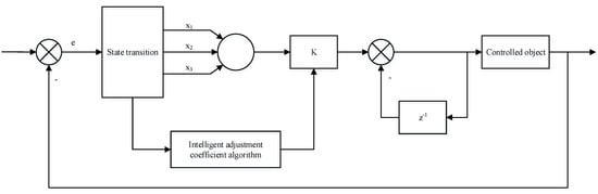
Figure 8.
Single neuron adaptive PID control structure.
Where , , and . Neurons generate control signals through correlation search 15:
where is the weight coefficient corresponding to . The controller achieved self-organization and self-adaptation by adjusting the weighted coefficient of network. The controller adjusts automatically using intelligent adjustment coefficient algorithm as follows [15]:
where is the steady-state initial value of proportional coefficient of neuron and is the adjustment coefficient, 1/10 of . The supervised Hebb learning rule was used. The Hebb learning rule is an unsupervised learning rule. The result of this learning is to enable the network to extract the statistical characteristics of the training set, thereby dividing the input information into several classes according to their degree of similarity. is the proportion coefficient of neuron, and its value is very important. The overshoot of will cause the system response overshoot; when the value is too small, the transition process becomes longer. In this study, the characteristics of valve opening flow are 5–40%, and the simulation and experiment showed that is 0.2. In the experiment, the supply air temperature set-point is 14 °C. The experimental data show that the control effect of the system is ideal, the system response is fast, the lag time is reduced, and the lag is eliminated.
3.4.2. Smith Predictive Control in Winter Condition
The principle of Smith pure lag compensation is as follows: Aiming at the delay characteristics of closed-loop system equations with pure time-delay terms, the controller was connected with one compensation link to make the closed-loop characteristic equation without pure delay to improve the control quality. Figure 9 shows the control principle [16].
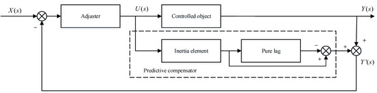
Figure 9.
Smith predictive control principle.
In Figure 9, the regulator transfer function is and the controlled object is . The transfer function of inertia element is and the pure lag is . is the predictor compensator transfer function introduced by Smith. The closed-loop transfer function can be expressed as follows:
The predictor compensator is located in the dashed box. Smith predictive control can eliminate the effect on the stability of closed-loop system caused by the pure lag between set-point and output value . The temperature control of supply air is based on Smith predictive PID control, as shown in Figure 10.
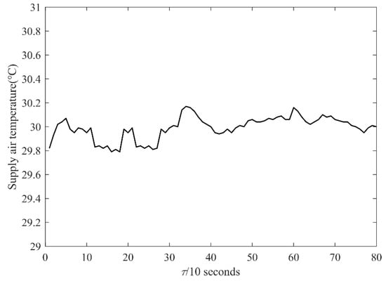
Figure 10.
Supply air temperature control effect.
At this time, the controller parameters are = 0.8, = 9 min, = 0.4 min, and the temperature of supply air is controlled at 30 °C. The system response is fast and the lag time is reduced. When the hysteresis is eliminated, the control effect is better, and the experiment requirement is satisfied.
4. Supply Air Temperature Optimization Control
Common supply air temperature set-point reset method: (1) Using the VAV terminal air valve opening signal as the indication signal for the relative load of each region, the supply air temperature was optimized in real time. (2) When the minimum or maximum air volume still cannot satisfy the requirements of room load, the supply air temperature was reset to adjust the room temperature. These two methods do not provide a specific numerical value for the optimal supply air temperature when the outdoor temperature is changed. In the past, the supply air temperature could be reset by using an advanced algorithm only. This is unfavorable to practical application of engineering. In this study, from an engineering standpoint, a large number of experiments were used to obtain the optimum supply air temperature.
4.1. Determination of Optimum Supply Air Temperature
All control links of the air-conditioning system are operated stably under closed-loop control. Based on the principle of minimum system energy consumption, certain fresh air volume is determined, and the outdoor temperature is obtained. Then, under this condition, the optimal supply air temperature of system is obtained. Furthermore, the relationship between outdoor temperature, indoor temperature, and supply air temperature is determined.
In the air-conditioning system, the experimental process of fresh air volume is shown in Figure 11. The process is applicable to all fresh air volume. In Figure 11, the fresh air volume was set according to GB 50736-2012 [17]. GB 50736-2012 is the Design Code for Heating Ventilation and Air Conditioning of Civil Buildings. Under different conditions, the fresh air volume is no less than 10% of the total supply air. First, by determining whether the outdoor temperature changes, the set-point of indoor and air temperature was kept constant. If the indoor temperature set-point is changed, the supply air temperature set-point is kept unchanged; otherwise, the air temperature set-point will change. According to this experimental method, the data under different fresh air conditions can be collected to determine the optimal supply air temperature set-point.
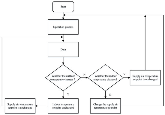
Figure 11.
Climate compensation experimental process under the minimum fresh air volume.
4.2. Analysis of Experiment
4.2.1. Analysis in Summer Condition
Analysis of Optimal Supply Air Temperature Set-Point
According to GB 50736-2012, the corresponding indoor temperature range is 24–26 °C in the heat comfort class II in summer. The maximum supply air temperature difference should not be greater than 10 °C in a comfortable air-conditioned room, and the temperature range of supply air temperature is 12–15 °C.
In the summer condition, the main energy consumption equipment for climate compensation test is a water chiller, secondary pump, and blower. In the case of fresh air volume, the outdoor temperature and indoor temperature set-points are constant. The supply air temperature set-point and the total energy consumption of system are a two-dimensional (2D) function, and extreme points must be present.
As shown in Table 2, the fresh air volume is constant; the outdoor temperature is 30.5 °C; the indoor temperature is 24 °C; the specific energy consumption of each frequency conversion device varies under different supply air temperatures. Table 2 shows that the lower the frequency of fan and secondary pump, the less the energy consumption. The total energy consumption of system first decreases and then increases with the change in the set-point of supply air temperature. When the supply air temperature is 13 °C, a minimum total energy consumption was observed. The energy consumption is 5.022 kW, including the chiller, secondary pump, and blower. The supply air temperature corresponding to this condition is the optimal supply air temperature set-point.
Table 2.
System energy consumption changes under different supply air temperatures.
The nonoptimal state of the table was selected for comparison. When the supply air temperature set-point is 12 °C, the total energy consumption of system is 5.350 kW. Compared with this point, the energy-saving rate of the optimal system can reach 6.1%. This shows that the climate compensation method proposed in this paper is feasible. A large number of experiments and data analysis verified that an optimal air temperature control point exists for the minimum total energy consumption of system.
Effect of Different Outdoor Temperatures on the System
According to the above experimental method, the relationship between outdoor temperature and optimal supply air temperature can be obtained under the fresh air volume and indoor temperature set-point. As shown in Figure 12, each outdoor temperature (30–33.5 °C) and the optimal supply air temperature present a 2D function relationship when the fresh air volume is minimum, and the indoor temperature set-point is 24 °C. During the operation of an air-conditioning system, when the indoor temperature is constant, the set-point of supply air temperature can be changed according to the outdoor temperature, so that the energy consumption of system is always in the minimum state, thereby saving energy.
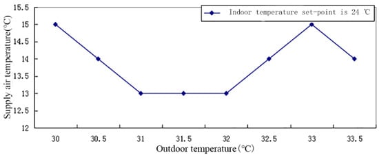
Figure 12.
Optimal supply air temperature when indoor temperature set-point is 24 °C.
Effect of Different Indoor Temperatures on the System
When the fresh air volume is constant and the indoor temperature set-point is changed, the relationship between outdoor temperature and optimal supply air temperature can be obtained using the same method as mentioned above. When the fresh air volume and indoor temperature set-point are constant, the outdoor temperature and air temperature set-point are variable. The outdoor temperature, supply air temperature, and total energy consumption of system is a three-dimensional (3D) function. If the outdoor temperature, indoor temperature set-point, and optimal air temperature set-point are represented by a picture, it is a 3D figure, as shown in Figure 13. Because the indoor temperature set-point is different, the optimal supply air temperature set-point varies with the outdoor temperature. According to the outdoor temperature, the indoor temperature set-point can determine the optimal supply air temperature set-point in the current condition.
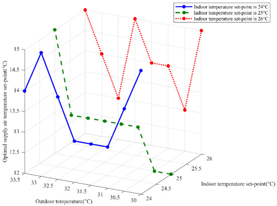
Figure 13.
Relationship between outdoor temperature and supply air temperature under different indoor temperature set-points.
4.2.2. Analysis in Winter Condition
According to GB 50736-2012, the heat comfort class II is used in winter, in which the indoor temperature range is 18–21 °C. When the outdoor temperature is 0 °C, the indoor temperature set-point is 19 °C. Figure 14 shows the relationship between system’s total energy consumption and supply air temperature. With the increase in supply air temperature, the total energy consumption of system reaches a minimum point, which is the optimal value of supply air temperature. Compared with the highest point, the optimal point has 35.5% energy saving in this experimental system. An optimal temperature point also exists for supply air under other operating conditions. By collecting each optimal supply air temperature under different conditions, Figure 15 shows the relationship curves between outdoor temperature and supply air temperature when the indoor temperature set-points are 19 °C, 20 °C, and 21 °C.
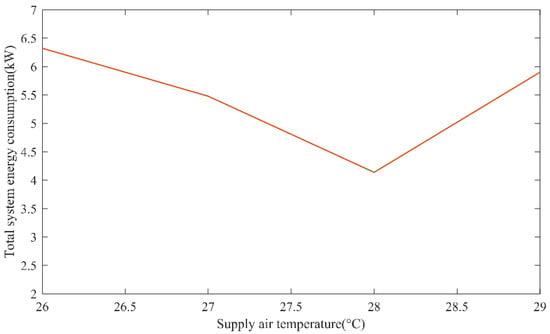
Figure 14.
Relationship between total system energy consumption and supply air temperature in winter condition.
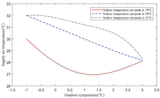
Figure 15.
Relationship between outdoor temperature and supply air temperature in winter condition.
In Figure 14, with the increase of supply air temperature, there is a minimum point in the total energy consumption of the system, and the supply air temperature corresponding to this point is the optimal supply air temperature under this condition. Under other working conditions, there is also the corresponding optimal supply air temperature. In this experimental system, the system can save 35.5% more energy in the operation of the optimal supply air temperature than in other operating conditions. In Figure 15, indoor temperature set-points are 19 °C, 20 °C, and 21 °C. Under the same indoor temperature set-point, the higher the outdoor temperature is, the lower the corresponding air supply temperature is, and the power consumption of the system is reduced. When the indoor temperature set-point increases by 1 °C, the corresponding supply air temperature increases under the determined outdoor temperature, and the system power consumption increases. Therefore, properly reducing the indoor temperature set-point can reduce the air supply temperature, and the power consumption of the system will be reduced to achieve the goal of energy saving.
5. Indoor Temperature Measurement Point Layout
5.1. Arrangement of Indoor Temperature Measuring Point
The physical model of this study is ROOM 5 of VAV laboratory of Xi’an University of Architecture and Technology. It is built from a heat-insulating steel plate in a large room and less affected by the external environment than a normal room. Its dimension is length (Y) × width (X) × height (Z) = 2.68 m × 2.36 m × 2.40 m.
According to ASHRAE 55-2010 [18], a reasonable space thermal environment is acceptable to occupants, considering the thermal environmental factors affecting the human body’s thermal sensation, indoor air temperature, humidity, airflow velocity, and average radiant temperature, but not considering personal factors affecting the comfort of human body [19]. The temperature difference optimizes the supply air temperature, changing the room temperature and comfort of indoor staff.
External windows are present on the wall, and the measurement should be 1.0 m inward from the largest central window. In any case, the environment should be predicted in the most extreme thermal condition such as around windows, mixed windows, corners, and entrances. At the same time, the measuring point should be far enough away from the boundary, and a sufficient space is available on any measuring sensor surface allowing full circulation. ASHRAE still recommends that when measuring the air temperature and air flow rate, one should consider sitting on the human ankle 0.1 m, wrist 0.6 m, and head 1.1 m; one should also consider standing human ankle 0.1 m, wrist 1.1 m, and head 1.7 m. According to the survey, the most sensitive part of indoor office staffs’ blowing feeling and comfort is at the plane of desk level. Therefore, the indoor air blowing feeling and comfort are fully considered, and a measurement plane of 1.9 m was set.
The temperature sensor layout planes are 0.1 m, 0.6 m, 0.75 m, 1.1 m, 1.7 m, and 1.9 m.
The room has an area of 6.32 m2, and the walls on both sides are glass walls. This is an extreme environment. For temperature measurement, the following areas were selected: Near the window area, corner, supply air outlet, air outlet, and return air outlet. Figure 16 shows the arrangement of temperature measurement points in the room. The same horizontal sensor numbers were used: 3-2, 3-3, 3-4; 2-2, 2-3, 2-4; 1-3, 1-4.
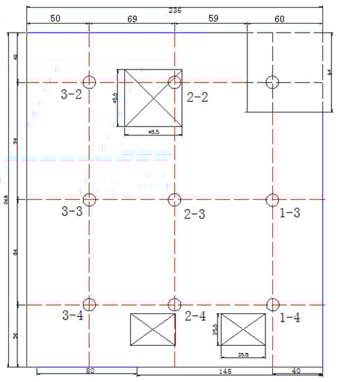
Figure 16.
Sensor installation.
The room physics model established by Gambit software was meshed to generate 113,944 grids, and the temperature sensitive parts were encrypted, as shown in Figure 17.
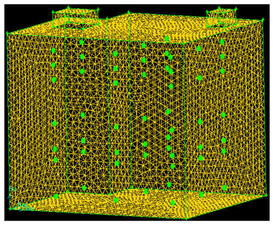
Figure 17.
Mapped meshing of physical model.
5.2. Setting of Operating Boundary Conditions
The entrance is the air supply outlet at the terminal of the air conditioning system, and the boundary is defined as the speed entrance (VELOCITYINL). The speed and temperature of supply air were assigned according to the experimental results measured using a temperature sensor and wind speed sensor at the terminal of the air conditioning system, 0.188 m/s, 0.388 m/s, and 0.588 m/s.
The exit is the return air inlet of air conditioning, and its boundary is defined as the exit (OUTFLOW). The wall surface is the solid wall of room, and it is a smooth wall. Its boundary is defined as the WALL. The setting of boundary conditions is as shown in Table 3.
Table 3.
Setting of boundary conditions.
5.3. Simulation of Indoor Temperature Distribution
In FLUENT, the temperature distribution of several different layers of 0.10 m, 0.60 m, 0.75 m, 1.10 m, 1.70 m, and 1.90 m in the room was simulated. Figure 18 shows the simulation results when the indoor temperature setting value is 26 °C and the supply air speed is 0.188 m/s.
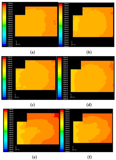
Figure 18.
Indoor temperature distribution nephogram while the wind velocity v = 0.188 m/s (a) z = 0.10 m temperature nephogram; (b) z = 0.60 m temperature nephogram; (c) z = 0.75 m temperature nephogram; (d) z = 1.10 m temperature nephogram; (e) z = 1.70 m temperature nephogram; (f) z = 1.90 m temperature nephogram.
Figure 18 shows that when the temperature and speed of indoor supply air temperature are constant, some plane temperatures are different. The air outlet temperature is slightly lower than the return air temperature; z = 0.10 m plane temperature > z = 0.60 m plane temperature > z = 0.75 m and 1.10 m plane temperature; z = 1.70 m and 1.90 m plane temperature value distribution layer is relatively large. Around the air supply port, the room center temperature has the second place. The return air outlet ambient temperature around the room is high; the wall temperature is the highest in the plane of z = 1.90 m. Simulation analysis shows that the temperature plane can reflect the indoor temperature distribution.
5.4. Analysis of Experimental Data of Indoor Temperature Measurement Points
The indoor temperature of the air-conditioned room under different working conditions was tested. The results are shown in Table 4.
Table 4.
Indoor supply air conditions.
By dealing with the indoor temperature detection value of the air-conditioning system under different supply air wind velocities while maintaining the indoor temperature constant, the room temperature of different layers is shown in Table 5, Table 6, Table 7 and Table 8 under different working conditions.
Table 5.
Indoor temperature at different levels under condition A.
Table 6.
Indoor temperature at different levels under condition B.
Table 7.
Indoor temperature at different levels under condition C.
Table 8.
Indoor temperature at different levels under condition D.
Table 5, Table 6, Table 7 and Table 8 show that in the measured temperature plane, the temperature sensor with an indoor height of 0.1 m has the lowest detection value. The temperature sensor detection values of indoor heights of 0.6 m and 0.75 m are centered. The temperature detection values of different sensors on each plane are also different. While maintaining the steady state of indoor temperature, it was observed that the temperature values of different horizontal levels in the room are different under the same working conditions in the room.
Table 9 and Table 10 show that the indoor temperature varies under different working conditions at the same level in the room. From the temperature data of different levels, it can be observed that the temperature sensor detection value of any plane with a higher supply frequency is smaller than the sensor detection value of the corresponding lower air supply frequency. In the temperature plane of 1.9 m only, when the air supply frequency is 50 Hz, the 3-2 sensor detection value is smaller than the air supply frequency of 45 Hz.
Table 9.
Different supply air velocities and indoor temperatures at 0.75 m.
Table 10.
Different supply air velocities and indoor temperatures at 1.1 m.
6. Determination of Indoor Temperature Optimal Measuring Point
Multisensor information fusion is the integration of data information provided by various sensors in the system to form a more reliable determination of the surrounding environment. Even if environment changes and some parts of the system have technical failure or damage, a more reliable determination can also be obtained for the surrounding environment. The difference between the obtained temperature fusion value and the actual value of indoor temperature sensor was obtained, and the absolute value was obtained. The sensor position corresponding to the absolute value is the optimal measurement point of room.
6.1. Determination of Indoor Optimal Measuring Point
The essence of multi-sensor information fusion is to imitate the way the human brain works, and comprehensively process the method from the combination of external information. Multiple sensor detection values are analyzed and processed in a certain way to make decisions. This kind of decision information is not independently obtained by any single sensor, thus forming a more reliable judgment of external information. The fusion temperature is obtained by fusing the temperatures measured by multiple sensors.
For multi-sensor systems, the core issue is to select the right fusion algorithm. The adaptive weighted average data fusion algorithm does not require prior knowledge and only requires the current measurement data obtained from the sensor [19]. The implementation of the fusion temperature by using adaptive weighted data fusion algorithm. Adaptive weighted fusion is to find the optimal weighting factor in an adaptive form according to the measured value of each sensor of the system under the condition that the total mean square error of the system is kept to a minimum, so as to achieve the optimal fusion result. Therefore, an adaptive weighted data fusion algorithm was used in this study. All the sensors are numbered as shown in Table 11.
Table 11.
Correspondence table between each sensor and actual position.
The measured values of different temperature sensors under different working conditions can be used to obtain the temperature fusion value under each working condition using adaptive weighted fusion algorithm. Furthermore, the location of sensor with the smallest absolute value can be obtained. The measured value of sensor with the smallest deviation is between the fusion value and true value, and the corresponding sensor position is the optimal measuring point of indoor temperature, i.e., , where is the number of sensor and is the data of th measurement of sensor. The results are shown in Table 12.
Table 12.
Data fusion results.
6.2. Indoor Temperature Simulation Control
By combining the abovementioned temperature measuring point fusion process with the control process, a multi-sensor control block diagram of the indoor air temperature of VAV air conditioning system is proposed for a pressure-independent end control device, as shown in Figure 19.
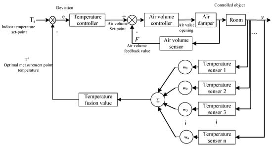
Figure 19.
Multisensor indoor temperature control block diagram.
A proportional-differential controller can correct the large-lag system in advance, so that the system adjustment is more stable. In this study, a PD (proportional-derivative) gain adjustable model reference adaptive system was used to evaluate the optimal temperature control. The PD gain adjustable model reference adaptive control system is mainly composed of a reference model, a controlled object, an adaptive control loop, and a conventional feedback controller [19], as shown in Figure 20.
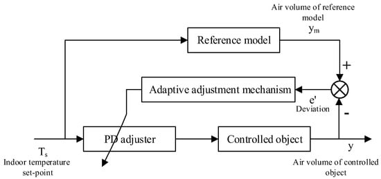
Figure 20.
PD gain adaptive regulation model block diagram.
As shown in Figure 20, the set-point is deviated from the output of controlled object by using the output of reference model, and the deviation is passed through the output signal of adaptive adjustment mechanism and then applied to the controlled object using the PD regulator until the deviation is equal to zero.
According to the terminal system equipment process, the input and output data of the air volume model and room temperature model are not observable, and the model of air volume controller is known by the manufacturer.
The indirect identification method was used to identify the closed loop model of outer loop and inner loop. The obtained object model and inner loop model were used as reference models for this control study, as Equations (10) and (11).
According to the block diagram analogy, the inner loop end model and room model are controlled object models, as Equations (12) and (13).
According to the reference model and controlled object model, Simulink was used to simulate the model-adaptive indoor temperature double closed-loop control system based on the PD gain adjustable model. Figure 21 shows the simulation results.
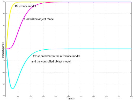
Figure 21.
Output curve comparison in terminal control system.
Figure 21 shows that the reference model reaches a steady state after the system runs for 50 s, and the controlled object model reaches a steady state after the system runs for 200 s. The deviation in the output of reference model obtained from the output of controlled object model is equal to zero at 200 s, at which point the end control system is progressively stable.
Table 13 shows the performance indicators of reference model and controlled object model.
Table 13.
Comparison of parameters of models.
Table 13 shows that the reference model and controlled object model are well selected, and the control system works well. This algorithm can be used for studying the optimal temperature control.
The VAV air-conditioning system adaptively adjusts the system according to the output deviation of reference model and controlled object model. Table 14 shows the performance of adaptive adjustment parameters.
Table 14.
Comparison of parameters of regulator adjustment.
Using MATLAB, the indoor temperature control was simulated by using the measured temperature of indoor temperature optimal measuring point and the nonoptimal measuring point as the feedback value under certain working conditions. The optimal indoor measuring point (26.193 °C) and two nonoptimal measuring points (25.943 °C and 27.543 °C) control output curves were compared. The indoor temperature was controlled using PD gain adjustable model and reference adaptive method. Table 15 shows a comparison of simulation control operation results.
Table 15.
Comparison of temperature simulation operation of optimal temperature and ambient temperature.
Table 15 shows that the adjustment time of indoor temperature controlled by the optimal measuring point is less than two nonoptimal measuring points. While effectively reducing the adjustment time, the system running time can also be reduced, thereby reducing the system energy consumption.
7. Conclusions
In this study, the climate compensation concept in the HVAC system was introduced into the air-conditioning system, and the principle of minimum total energy consumption was used to find the best advantage of supply air temperature. Experiments show that the proposed method can be used to achieve the optimal supply air temperature. According to the best advantage of the measured supply air temperature, appropriate control strategies and methods can be used to compensate the climate change and reduce the impact of climate change on the system.
Furthermore, the temperature measurement points of an VAV terminal system were simulated, focusing on the scientific arrangement of multi-sensor measuring points in the air-conditioned room and the accuracy of indoor temperature measuring points and the actual temperature of each plane temperature sensor under different working conditions. The detection value, the absolute value of same data fusion, was applied to obtain the optimal measurement point of indoor temperature. The optimal measurement point of indoor temperature was found at the height of 0.65 m and 0.7 m. Simulation shows that the optimal point of indoor temperature is better than the control of nonoptimal measuring point. This provides a reference for the control of optimal measuring point of indoor temperature in a VAV air conditioning system. The arrangement of temperature sensor is subjective. If the temperature sensor can be arranged by an intelligent algorithm, the control effect on the optimal measuring point of indoor temperature will be more obvious.
- (1)
- The optimal supply air temperature was obtained through experiments in this study and belongs to the engineering optimization method with engineering practicability.
- (2)
- Under the premise of satisfying indoor requirements, when the outdoor temperature increases, the indoor temperature set-point can be appropriately reduced to save energy consumption.
- (3)
- With the change in outdoor temperature, by adjusting the optimal supply air temperature in real time, the minimum energy consumption of system can be maintained.
- (4)
- For the initial study on the optimal indoor temperature measuring point, this study limits the indoor temperature optimal measuring point position to two levels. Further studies can be conducted to optimize this optimal point to only one point. Follow-up studies can consider the indoor effective air blowing temperature, i.e., combine the optimal indoor temperature measurement point with the optimal wind speed measurement point to improve the comfort of indoor personnel. The selection and placement criteria of the optimal measuring points can be summarized, so that the sensors can be arranged according to this standard in any air-conditioned room.
Author Contributions
Conceptualization and methodology, X.Y.; numerical simulation and data analysis, M.L. and A.H.; paper writing, M.L., A.H., and C.L. Review and revision of papers, X.Y. and C.L.; resources and supervision, K.F. and Q.M. All the authors provided comments and suggestions for the writing and descriptions in the manuscript.
Funding
This study was supported by the National Natural Science Foundation of China (Grant No. 51508446) and the Key Research and Development Plan Project of Shaanxi Province (Grant No. 2017ZDXM-GY-025).
Conflicts of Interest
The authors declare no conflict of interest.
References
- Xiao, C.; Fu, L. Discussion on weather compensators applied to heating systems. Heat. Vent. Air Cond. 2007, 37, 136–140. [Google Scholar]
- Chen, L. Application of climate compensator in heating system. Build. Sci. 2010, 26, 42–46. [Google Scholar]
- Li, X.; Zhou, H. Analysis on energy-saving retrofit of the climate compensation in a university. Energy Conserv. 2015, 4, 58–61. [Google Scholar]
- Cui, J.; Qin, Y.; Wang, R.; Li, W.; Zhang, W.; Li, X. Post evaluation on building energy-saving reconstruction for a hospital in Beijing. Build. Sci. 2017, 33, 79–84. [Google Scholar]
- Ke, X.; Ke, Y. Central Air-Conditioning Climate Compensation Controller and the Central Air-Conditioning Climate Compensation Method. China Patent 101650063, 17 February 2010. [Google Scholar]
- Zhang, W.; Shen, X.; Yu, H.; Han, L.; Hu, P.; Ma, J.; Zhao, D.; Chen, Z.; Wang, X.; Wang, M. Energy-Saving Method for Heating and Returning Water Temperature Control with Integrated Climate Compensation. China Patent 101737847A, 16 June 2010. [Google Scholar]
- Engdahl, F.; Johansson, D. Optimal supply air temperature with respect to energy use in a variable air volume system. Energy Build. 2004, 36, 205–218. [Google Scholar] [CrossRef]
- Jin, X.; Xia, Q.; Zhou, X.; Wang, S. Online control strategies of supply air temperature for multi-zone VAV air-conditioning system. J. Shanghai Jiaotong Univ. 2000, 34, 507–512. [Google Scholar]
- Liu, Q.; Du, Z.; Jin, X. A study on the effect of location of indoor temperature sensor’s of VAV air conditioning system. Build. Energy Environ. 2013, 32, 11–14. [Google Scholar]
- Cai, P.; Li, L.; Zeng, L. Study and simulation to the optimal supply air temperature in AHU systems. Energy Conserv. Technol. 2017, 35, 349–354. [Google Scholar]
- Song, Q.; Liu, Y.; Ma, Y.; Tan, Y. Design of temperature and room temperature and humidity control system based on multi-sensor data fusion. Jiangsu Agric. Sci. 2015, 43, 394–396. [Google Scholar]
- Kojima, K. Study on sensor fusion for detecting human’s thermal comfort considering of individuals. In Proceedings of the 2010 10th International Conference on Intelligent Systems Design and Applications, Atlanta, GA, USA, 23–25 August 2010; pp. 1355–1360. [Google Scholar]
- Ge, X.; Du, Z.; Jin, X. Investigation of variable air volume optimal control for air conditioning system based on multi-sensor data fusion. Chin. J. Refrig. Technol. 2016, 36, 28–33. [Google Scholar]
- Lu, J.; Ma, Z.; Zou, P. HVAC; China Building Industry Press: Beijing, China, 2008. [Google Scholar]
- HOU, Y.; Guo, W. Research on design of single neural element self-adaptive PID controller. Microcomput. Inf. 2005, 21, 8–9. [Google Scholar]
- Wang, Z.; Liu, H.; Chen, Y. Process Control System and Instrument; China Machine Press: Beijing, China, 2006. [Google Scholar]
- GB 50736-2012. Design Code for Heating Ventilation and Air Conditioning of Civil Buildings; The Standardization Administration of China (SAC): Beijing, China, 2012. [Google Scholar]
- ANSI/ASHRAE Standard 55-2010. Thermal Environmental Conditions for Human Occupancy Includes ANSI/ASHRAE Addenda Listed in Appendix I; ANSI: New York, NY, USA, 2010. [Google Scholar]
- Xu, X.; Li, B. Influence of indoor thermal environment on thermal comfort of human body. J. Chongqing Univ. Nat. Sci. Ed. 2005, 28, 102–105. [Google Scholar]
© 2019 by the authors. Licensee MDPI, Basel, Switzerland. This article is an open access article distributed under the terms and conditions of the Creative Commons Attribution (CC BY) license (http://creativecommons.org/licenses/by/4.0/).