Article

New Fast MPPT Method Based on a Power Slope Detector for Single Phase PV Inverters

Department of Electrical Engineering, University of Valencia, Avd. Universitat S/N, 46100 Burjassot-Valencia, Spain
*
Author to whom correspondence should be addressed.
Energies 2019, 12(22), 4379; https://doi.org/10.3390/en12224379
Submission received: 21 October 2019 / Revised: 7 November 2019 / Accepted: 15 November 2019 / Published: 18 November 2019
(This article belongs to the Section A2: Solar Energy and Photovoltaic Systems)

Abstract

:
This article presents a novel MPPT method for two stage PV inverters with a single phase connection to the power grid. The method takes advantage of the 100 Hz/120 Hz harmonic present on the DC-bus voltage to guide the MPP search. It consists of detecting the slope of the P-V curve and integrating it to obtain the duty-cycle. The power slope detector (PSD) is able to calculate the P-V slope to command the MPPT even at very low powers, where the amplitude of the oscillations is barely perceptible. Design equations are provided, both of the gain of the PSD and of the gain of the MPPT integrator. It also shows how this PSD-MPPT strategy can be combined with the power control, allowing regulation of powers lower than those of the MPP. The power control loop is analyzed, and its stability is related to a single gain to be designed. The PSD-MPPT is tested in a two stage PV inverter, where the step-up DC-DC converter consists of three parallel boost converters. The results show that the PSD-MPPT method can work without the measurement of the current in the boost converters, which implies a cost reduction. A PV efficiency of about 99.8% is obtained with a usual ripple in the DC-bus of 4% peak-peak. In addition, the PSD-MPPT method is characterized as being extremely fast, both in the MPP search and in the power control, with response times around 50 ms. The PSD-MPPT is a simple algorithm of constant parameters that can be solved in a low cost microcontroller at a sampling frequency of about 2 kHz, requiring only the voltage and current of the PV array.

Graphical Abstract

1. Introduction

Photovoltaic (PV) inverters are DC-AC converters that allow the extraction of photovoltaic energy from solar panels and its injection to the power grid or any 50/60 Hz AC-bus. They are used in commercial solar plants for high power production, where the PV inverters feed the energy directly to the grid or in solar home systems where the PV inverter feeds the household AC loads connected at its output. In the first case, the AC output of the PV inverter acts as a controlled current source, whereas in the solar home application, the AC output can also operate as a voltage source to create the AC-bus voltage when islanding operation is detected.
The topological structure of the PV inverter depends on the power and voltage levels generated by the array of solar panels. When the power of the array is greater than 6 kW, as happens in commercial solar plants, three phase grid connected inverters [1,2] are used. For lower powers, as in the case of solar home systems, single phase inverters [3,4,5,6] are used. On the other hand, the input voltage of the PV inverter depends on the number of solar panels connected in series. In this sense, we can distinguish the concepts of the micro-inverter, string-inverter, and central-inverter. The micro-inverter is designed to be connected to only one solar panel and therefore is rated for low input voltage and low power. The string-inverter is designed for higher input voltage levels, which are achieved by connecting an array of panels in series. The central-inverter is intended to connect a large number of panels in a parallel arrangement of strings, in order to generate higher power levels using a single piece of hardware and therefore at a lower price per kilowatt installed.
When PV voltage is low (less than about 400 V in single phase connection and 800 V in three phase), as occurs in micro-inverters and string-inverters, a DC-DC converter is included inside the PV inverter to raise the voltage on the DC-bus so that the inverter can operate. This step-up DC-DC converter is also responsible for adjusting the PV voltage to extract maximum power from the array using maximum power point tracking (MPPT) algorithms. On the contrary, if the PV voltage is high enough, the array of panels can be connected directly to the DC-bus without a DC-DC converter [1,4], and it is the inverter responsible for adjusting the bus voltage to search for the maximum power point (MPP).
In micro-inverters, string-inverters, and some central-inverters, the required step-up DC-DC converter is usually a boost converter [2,3,5] or a flyback [6], which also provides isolation between the photovoltaic panel and the grid. However, the inclusion of the step-up converter penalizes efficiency and reduces reliability, since a fault interrupts the harvest of PV energy until the module is replaced.
One solution to this problem is to build the step-up DC-DC converter using a parallel arrangement of N converters, as shown in Figure 1. When one of the converters fails, it is automatically disconnected by means of a relay, and the inverter continues to operate without the production of energy being stopped. In addition, the parallel interleaved solution improves the overall efficiency of the DC-DC converter and reduces the size of the input capacitors and magnetic components to be integrated into printed circuit boards (PCB) [7,8].
Regarding the MPPT method to be used in the parallel arrangement, it must allow a balanced sharing of the currents between the step-up converters, and of course, it must guarantee a high photovoltaic efficiency.
All MPPT algorithms need voltage variations in the PV array to guide the MPP search. These variations can be generated by the MPPT itself in the form of voltage steps, as in the perturb and observe (P&O) method [9,10,11] and incremental conductance (IC) method [12], or in sinusoidal form as in [13]. They can also use present oscillations not generated by the MPPT, such as in [14], where the transient oscillations of the input filter were used, or in [15], where the ripple of the PV voltage at the switching frequency was used.
In the case of PV inverters with a single phase grid connection, the inherent oscillating feature of the instantaneous power generated in the grid produces a 100/120 Hz oscillation in the DC-bus voltage. This oscillation makes it difficult to search for the MPP when the MPPT generates its own disturbance, as both overlap, producing search errors that decrease PV efficiency. To solve it, in [6], a current loop was implemented that prevents the propagation of the 100 Hz harmonic to the PV voltage. Although the method offers excellent performance, in the parallel layout, the inclusion of a current sensor and the current control itself in each step-up converter makes the solution more expensive.
As an alternative, this article proposes precisely to use the 100 Hz harmonic present in the DC-bus and in the PV voltage to guide the MPP search. The method is based on a recent publication [13], where a 40 Hz sinusoidal disturbance was introduced in the duty-cycle to resolve the MPPT in a PV step-down battery charger. To adapt this method to the PV inverter, the generation of the 40 Hz disturbance is dispensed with and only the 100 Hz harmonic is transmitted to the PV voltage. The challenge now is that the amplitude of this disturbance is not constant, as it decreases as the power delivered decreases. Essentially, the method is to detect the slope of the P-V curve and integrate it to determine the duty-cycle. The power slope detector (PSD) uses band-pass filters tuned to 100 Hz to detect the oscillations in power and voltage in the solar array and calculates the P-V slope even at low powers where the amplitudes of these oscillations are very small. In addition, an extension of the method is proposed that allows controlling powers lower than that of the MPP.
The PSD-MPPT method was tested on the prototype shown in Figure 2, formed by a parallel arrangement of three boost converters and a single phase inverter connected to the mains through a transformer. As will be seen later, the experimental results showed that the PSD-MPPT method presented settling times to the MPP or to the power reference of around 50 ms and gave a PV efficiency of 99.77% at maximum irradiance with a voltage ripple in the DC-bus of 4% peak-peak. Smooth variation of the duty-cycle prevented current peaks, and balanced currents could be achieved without using a current control, resulting in a reduction of the manufacturing cost. Moreover, it was possible to activate and deactivate converters as a solution for reliability and to improve efficiency, without producing current peaks or modifying operation at the MPP.

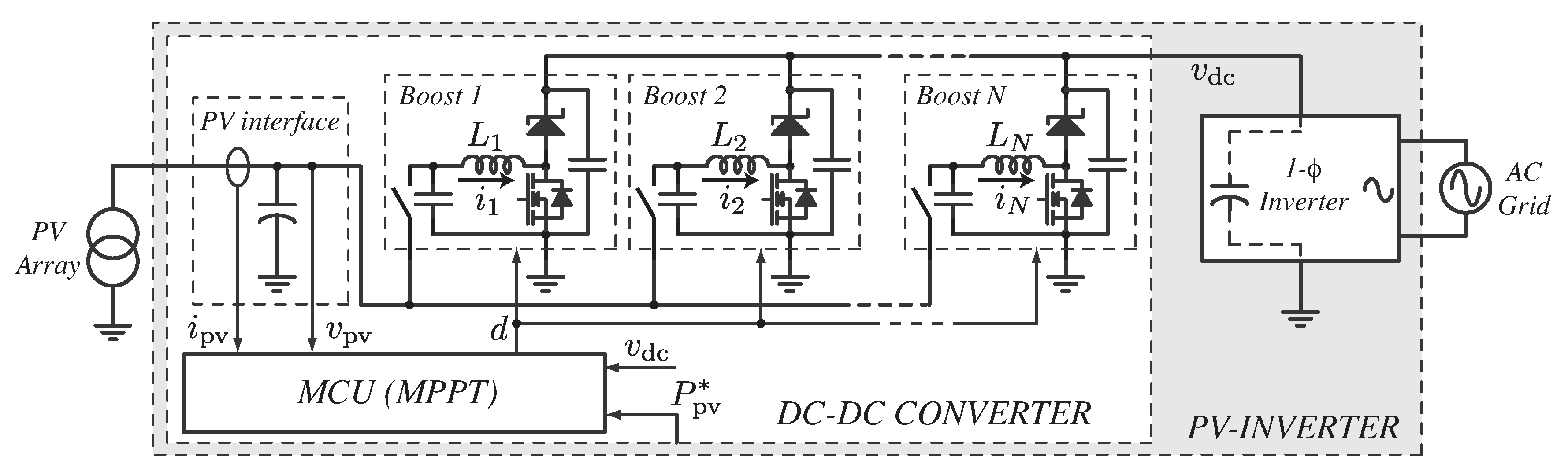
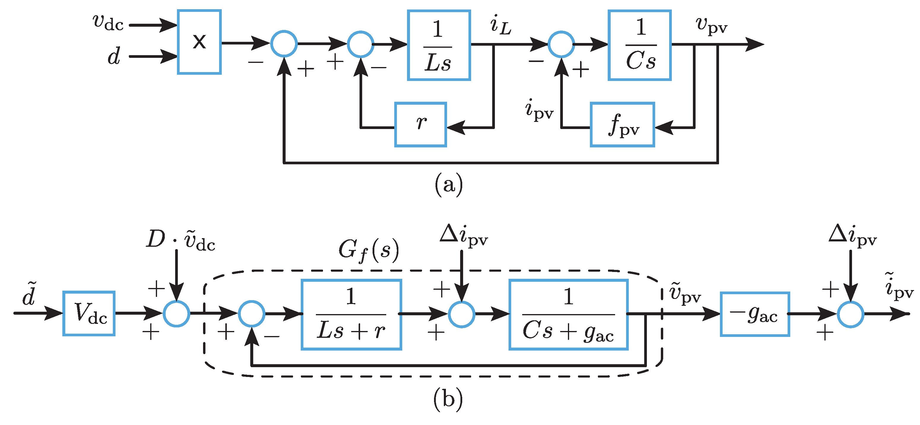
2. Converter Modeling

It was assumed that all parallelized boost converters in Figure 2 were identical, i.e., they contained the same inductors ( L 1 = L 2 = L 3 L j ) and power devices, and received the same gate drive signals. In this case, the voltages applied to all inductors were approximately equal, and hence, inductors could be assumed to be in parallel. As a consequence, the parallel arrangement of converters in Figure 2 could be modeled as a single boost converter with an inductance L L j / n and the inductor’s equivalent series resistance (ESR) r r j / n , where n 3 is the number of active converters and r j is the ESR of each individual inductor, the equivalent inductor current being i L j n i j .
Figure 3a shows the large-signal averaged model of the equivalent boost converter in continuous-conduction mode (CCM), where for convenience, d denotes the diode’s duty-cycle. The function f pv contains the characteristic I-V curves of the PV panel and gives the current i pv for a given irradiance and voltage v pv . Figure 3b presents the converter small-signal model or AC model, where DC values are expressed in capital letters. Δ i pv stands for a variation in the PV current due to a change in irradiance, and thus, the full variation is given by i ˜ pv = Δ i pv g ac · v ˜ pv , where g ac d i pv d v pv is the incremental conductance of the PV module. The transfer function G f can be approximated as:
G f ( s ) 1 ( s ω n ) 2 + 2 ζ ( s ω n ) + 1
where the natural frequency is ω n = 1 / L C and the damping factor is ζ = ( r / Z b + g ac Z b ) / 2 with Z b L / C .

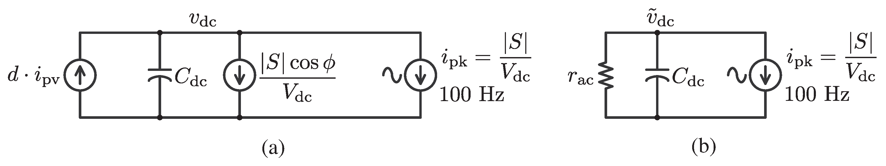
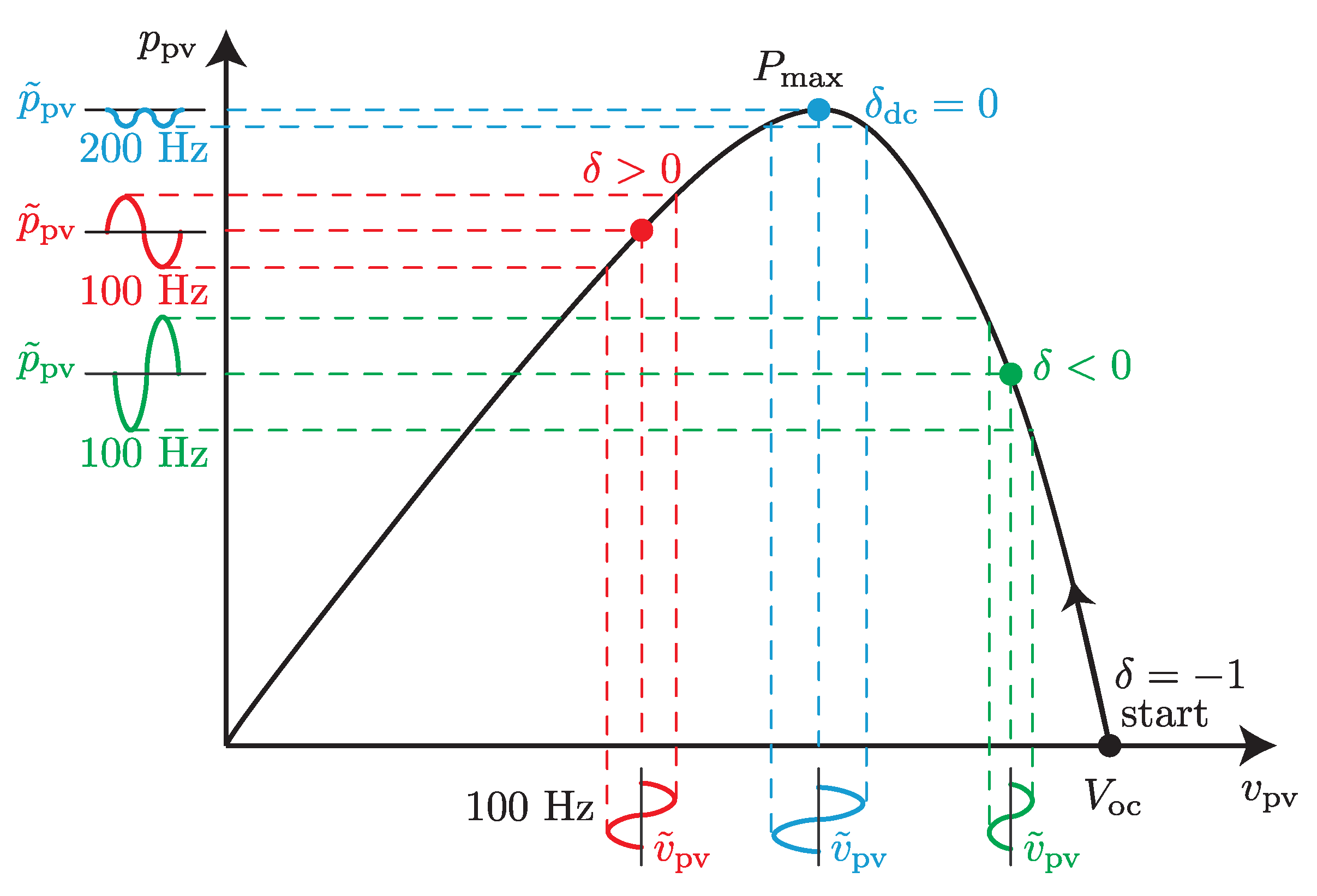
3. DC-Bus Voltage Modulation and PV Efficiency

The instantaneous power p g injected to the grid by a single phase inverter is:
p g ( t ) = v g p k · cos ( ω g t ) · i g p k · cos ( ω g t + ϕ ) = | S | · cos ϕ + | S | · cos ( 2 ω g t + ϕ )
where v g p k and i g p k are the peak amplitudes of the grid voltage and current, respectively, ω g is the grid frequency, S is the apparent power handled by the inverter, and ϕ is the voltage-current angle. This fluctuation of the instantaneous power generates a modulation v ˜ dc in the DC-bus voltage at frequency 2 ω g (100 Hz in this case), as illustrated in Figure 4. Neglecting the duty-cycle oscillations at 100 Hz, which will be attenuated by a proper control design, and taking into account Figure 3b, the DC-bus voltage modulation v ˜ dc generates the PV voltage oscillation v ˜ pv = D · v ˜ dc , as G f | 100 Hz 1 . The DC-bus charging current d · i L d · i pv is also modulated, which is accounted for by means of r ac in the AC model given in Figure 4b, where:
r ac = v ˜ dc D · i ˜ pv = 1 D 2 g ac
Since 2 ω g r ac C dc 1 , the amplitude of the DC-bus oscillation can be calculated as:
v ˜ dc p k = | S | V dc C dc 2 ω g
Considering the small-signal decompositions v pv = V pv + v ˜ pv and i pv = I pv + i ˜ pv , the generated PV power can be expressed as:
p pv = v pv · i pv = V pv · I pv + d p pv d v pv · v ˜ pv g ac · v ˜ pv 2
where d p pv d v pv = V pv ( g dc g ac ) is the P-V slope and g dc I pv / V pv is the static conductance of the PV array.
Assuming a sinusoidal PV voltage variation:
v ˜ pv = v ˜ pv p k · cos ( 2 ω g t )
the PV power results:
p pv = P pv + p ˜ pv
being P pv = V pv · I pv ( v ˜ pv p k ) 2 · g ac / 2 , and:
p ˜ pv = d p pv d v pv · v ˜ pv p k · cos ( 2 ω g t ) ( v ˜ pv p k ) 2 · g ac / 2 · cos ( 4 ω g t )
Equation (8) indicates that power oscillates with the harmonics at frequencies 2 ω g (100 Hz) and 4 ω g (200 Hz). This can also be observed in Figure 5. When operating far from the MPP, the P-V slope is large and the 100 Hz term predominates in Equation (8). Conversely, at the MPP, the P-V slope is null and power oscillates at 200 Hz. These oscillations directly determine the PV static efficiency η P avg / P max .
Unfortunately, the small-signal approximation Equations (7) and (8) cannot accurately predict the amplitude of the power oscillation, nor the efficiency, as they do not consider the distortion in i pv produced by the I-V characteristic (Figure 6a). Instead, the efficiency can be approximated by:
η ( % ) 100 · ( P max + P ¯ min ) / 2 P max
where P ¯ min ( P min 1 + P min 2 ) / 2 , and the two minimum power values P min 1 and P min 2 can easily be obtained from the P-V curve at maximum irradiance as depicted in Figure 6b. Table 1 indicates the expected efficiencies for different oscillation amplitudes in the DC-bus voltage. In the present work, the bus capacitance C dc was designed using Equation (4) to get a 4% peak-peak ripple at nominal power, and therefore, the expected efficiency was around 99.8%. Since v ˜ pv / V pv = v ˜ dc / V dc , this led to v ˜ dc p k = 0.02 · V dc in the DC-bus and v ˜ pv p k = 0.02 · V MPP in the PV array at nominal power.

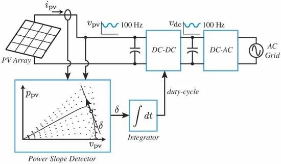
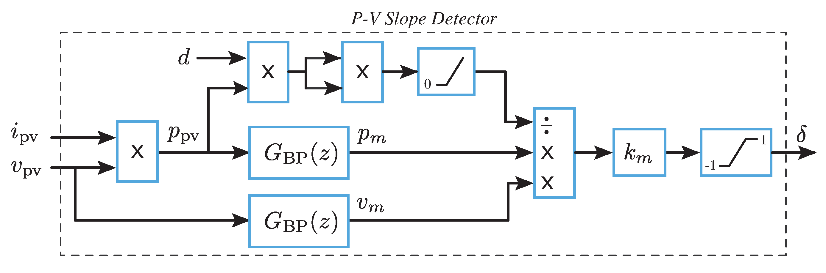
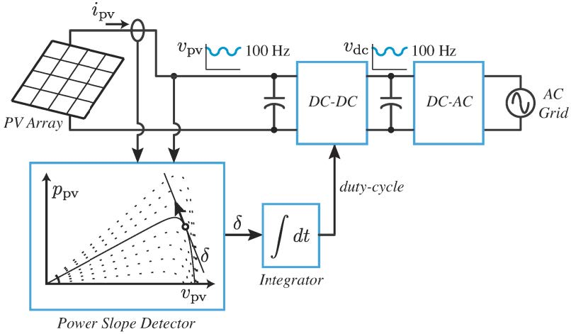
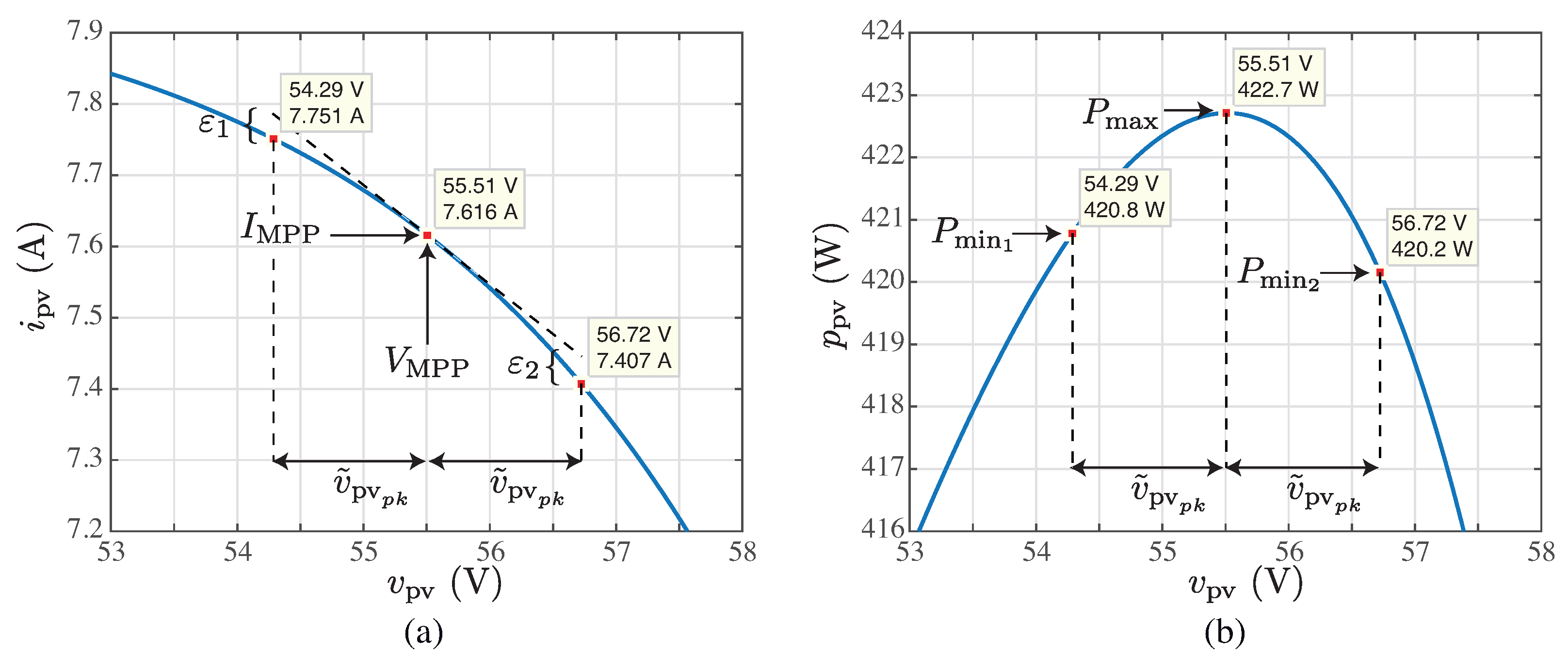
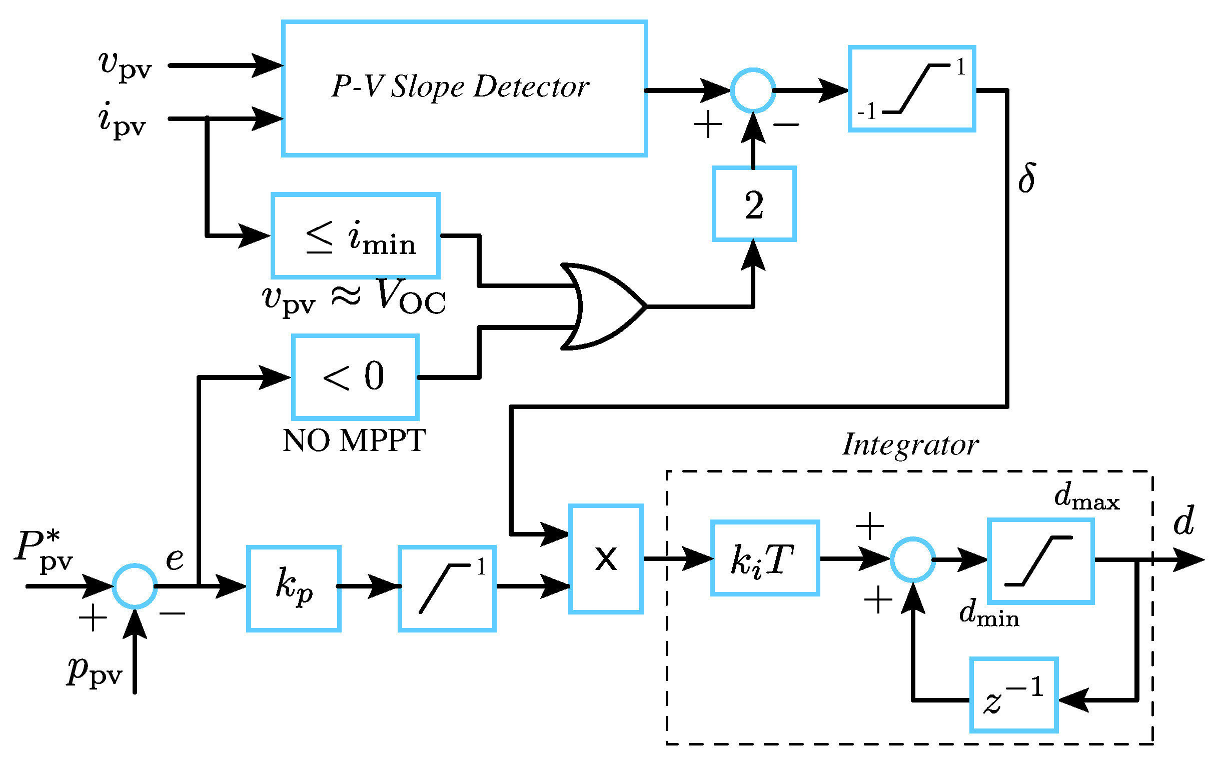
4. Proposed P-V Slope Detector

The MPPT method that will be presented in next section is based on the P-V slope detection to determine the direction and rate of change of the duty-cycle. The proposed strategy to obtain the P-V slope is similar to the product detector used for amplitude modulation (AM) demodulation. Indeed, by multiplying Equations (6) and (8), we get:
p ˜ pv · v ˜ pv = A · d p pv d v pv B · cos ( 2 ω g t ) A · d p pv d v pv · cos ( 4 ω g t ) B · cos ( 6 ω g t )
where A = ( v ˜ pv p k ) 2 / 2 and B = g ac ( v ˜ pv p k ) 3 / 4 , and taking the average value of Equation (10):
< p ˜ pv · v ˜ pv > = A · d p pv d v pv
we get a quantity proportional to the P-V slope. However, according to Equation (4), A presents a dependence on the power through:
A = 1 8 d · p pv V dc C dc ω g 2
To remove this dependency, it is proposed to solve the calculation p ˜ pv · v ˜ pv / ( d · p pv ) 2 . Figure 7 details the implementation of the power slope detector (PSD), where the AC components of PV power and voltage are obtained by means of the band-pass filters G BP , resulting in signals p m and v m , respectively. The PSD calculates:
δ = k m · p m · v m ( d · p pv ) 2
the averaged value of which is strictly proportional to the power slope:
δ dc < δ > = k m 8 V dc C dc ω g 2 · d p pv d v pv
It should be noted however that the slope detector output δ is not averaged and contains the frequency harmonics manifested in Equation (10). Out of the MPP, δ exhibits a mean value proportional to the slope and the dominant 200 Hz harmonic, while at the MPP, the mean value is zero and the 100 Hz and 300 Hz harmonics are visible (see Figure 9).
Constant k m is intended to fit calculated δ to the interval [ 1 , 1 ] . A good design criterion is to set k m so that δ dc is around 0.5 at the short-circuit region at maximum irradiance, which results however in a saturation to 1 when operating far to the right of the MPP. This gives the design equation:
k m = 4 V dc C dc ω g 2 I sc
where I sc is the short-circuit current at maximum irradiance.
The band-pass digital filters G BP ( z ) needed to extract the AC components of v pv and p pv were implemented using second-order all-pass filters G AP ( z ) as:
G BP ( z ) = 1 2 1 G AP ( z )
where:
G AP ( z ) = k 2 z 2 + k 1 ( 1 + k 2 ) z + 1 z 2 + k 1 ( 1 + k 2 ) z + k 2
with coefficients calculated as:
k 1 = cos ( ω 0 T ) k 2 = 1 tan ( ω BW T / 2 ) 1 + tan ( ω BW T / 2 )
for a given center-frequency ω 0 , bandwidth ω BW , and sampling period T = 1 / f s . Using ω 0 = ω BW = 2 ω g = 2 π 100 rad/s and f s = 20/11 kHz, the programmed all-pass filter results as:
G AP ( z ) = 0.7028 z 2 1.602 z + 1 z 2 1.602 z + 0.7028
and the band-pass filter is:
G BP ( z ) = 0.2972 ( z 1 ) ( z + 1 ) 2 z 2 3.204 z + 1.406
Figure 8a plots the Bode diagram of the band-pass filters. The center frequency is 100 Hz or 200 π = 628 rad/s. Notice that if grid frequency varies slightly, both signals v m and p m are shifted the same phase angle, and therefore, Equation (10) still holds. That is why the method can be implemented using constant parameters filters even if grid frequency varies.
Figure 8b presents the step transient response of the filters, showing their derivative behavior. This is especially important when filtering p pv , as the proposed MPPT allows a very fast change in power. The transient produced in p m takes a number of settling samples n s = 4 / log | P z | , where P z are the complex poles of G BP ( z ) . The transient settling time is t s = n s T = 12.5 ms. As shown in Figure 9, during these transients, the slope detector does not measure properly and presents saturations in δ .

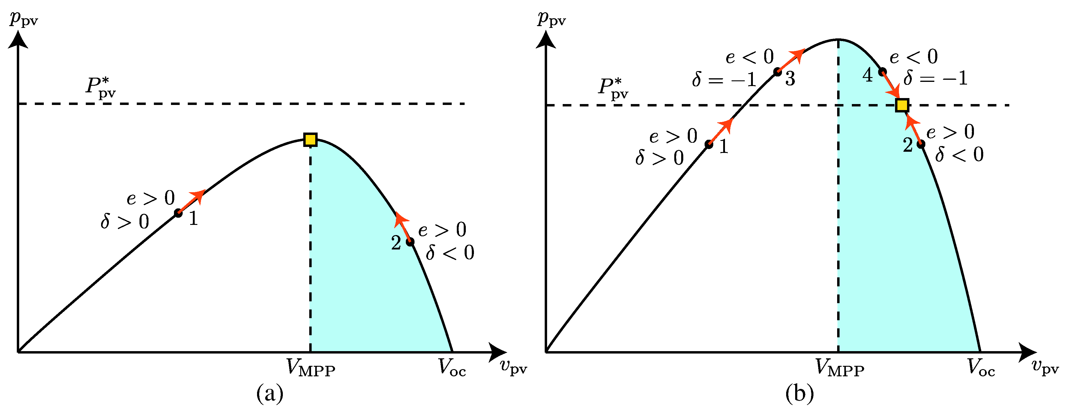
5. Maximum Power Point Tracking Based on the P-V Slope Detector

The proposed PSD-MPPT strategy is shown in Figure 10. The duty-cycle was obtained by a simple integration of δ . To the left of the MPP, δ dc is positive, and the duty-cycle increases. To the right of the MPP, δ dc is negative, and the duty-cycle decreases. As the converter approaches the MPP, δ dc tends to zero, and the duty-cycle slows down to finally get a still MPP operation.
The integrator’s gain k i has to be limited to prevent fast changes in PV voltage that excite the transients of the band-pass filters at their natural frequencies. The following equation limits the effect of a saturated oscillation in δ during a transient, of frequency 2 ω g , to a PV voltage oscillation of amplitude less than 1% of V MPP :
k i max = 2 π V MPP V dc
At the converter start-up, when the duty-cycle is high and the PV panel operates in open-circuit, the slope detector does not function since i pv = 0 . To solve this problem, the slope detector output is modified by setting δ to 1 only when i pv i min , that is when operation is close or at the open-circuit voltage. Notice that this is not a discontinuity in the value of δ , since the slope detector saturates to −1 when operating in the neighborhood of the open-circuit voltage.
An averaged switch model of the PV inverter shown in Figure 2 was simulated using PSIM©, with the proposed PSD-MPPT and parameters given in Table 2 and Table 3. Figure 11 shows the simulation results against irradiance step changes between 250 W/m 2 and 1 kW/m 2 every 125 ms. The figure shows, from top to bottom: i pv , v pv , p pv , currents i j through the inductors ( i 1 , i 2 , and i 3 ), p m and v m extracted by the band-pass filters, parameter δ , duty-cycle d, DC-bus voltage v dc , and the inverter’s output current and voltage. The converter starts up and takes only 50 ms to find the MPP at maximum irradiance. Every new MPP is found in approximately 50 ms. The calculated PV efficiency at maximum irradiance is η = 100 · 402.9 / 403.6 = 99.83 %. It should be noted that inductors currents i j show safe values and are equalized despite not using a current control on each converter module.

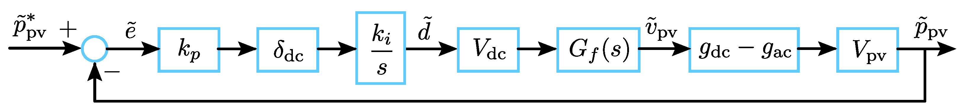
6. Modification for Power Reference Tracking

Though PV inverters usually operate in the MPP all the time, it may be necessary to generate power below the MPP [16], for instance when the inverter is in island mode without any chance of injecting the generated power to the main grid, the load demand is moderate, and batteries are in a high state of charge. Figure 12 presents the modified PSD-MPPT algorithm to achieve PV power control, where P pv is the power reference. Now, if the error signal e is negative, which indicates that the generated power is excessive compared to the reference, δ is set to −1, and since δ · e > 0 , the duty-cycle increases until a steady-state of regulated power is found to the right of the MPP.
Figure 13 illustrates the operating process in all possible scenarios. If the reference is higher than the actual power (Points 1 and 2), δ is not modified, and the converter climbs in power, as explained in the previous section. The speed of climbing is limited by the upper-limit saturator to meet the criteria given in Equation (21) and slows down when approaching the power reference. If the actual power exceeds the reference (Points 3 and 4), δ is set to 1 and the duty-cycle increases until the power lowers below the reference. In this case, the only possible stable point is to the right of the MPP (yellow point in Figure 13b).
The stability of the proposed power control was achieved through a single gain k p . Figure 14 shows the small-signal model of this control. It can be shown that the worst-case dynamics occurs when regulating a small power, thus near open-circuit operation ( δ = 1 ), at maximum irradiance and with only one active converter. Gain k p in Table 3 has been designed under these conditions to achieve the phase margin (PM) and gain margin (GM) shown in Figure 15a. When operating in any other condition, the stability margins are higher. For instance, Figure 15b shows the open-loop Bode diagram when operation is at the MPP with maximum irradiance and with all three converters active.
The proposed power control with PSD-MPPT was again simulated using PSIM©, and the results are presented in Figure 16 and Figure 17, both at maximum irradiance. Specifically, Figure 16 shows the control performance against reference steps between 200 W and 500 W. The converter takes approximately 50 ms to shift from medium power to MPP and vice versa. On the other hand, Figure 17 shows the simulation results against reference changes between 0 W and 500 W. This is a more challenging case, because the null power regulation at the open-circuit voltage presents the lowest stability margins and because duty-cycle transitions here are the widest possible. Transients take 70 ms from zero power to MPP and 25 ms from MPP to null power. It should be noted again that the currents i j of all three boost modules are equalized and do not present peaks during transients.

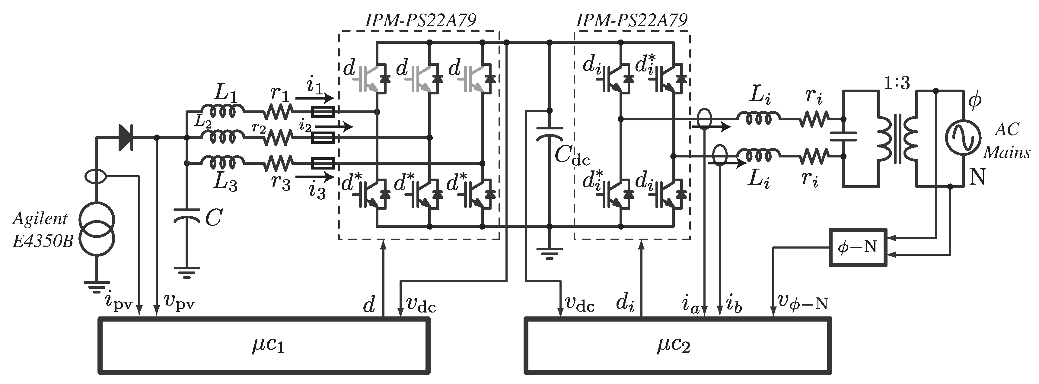
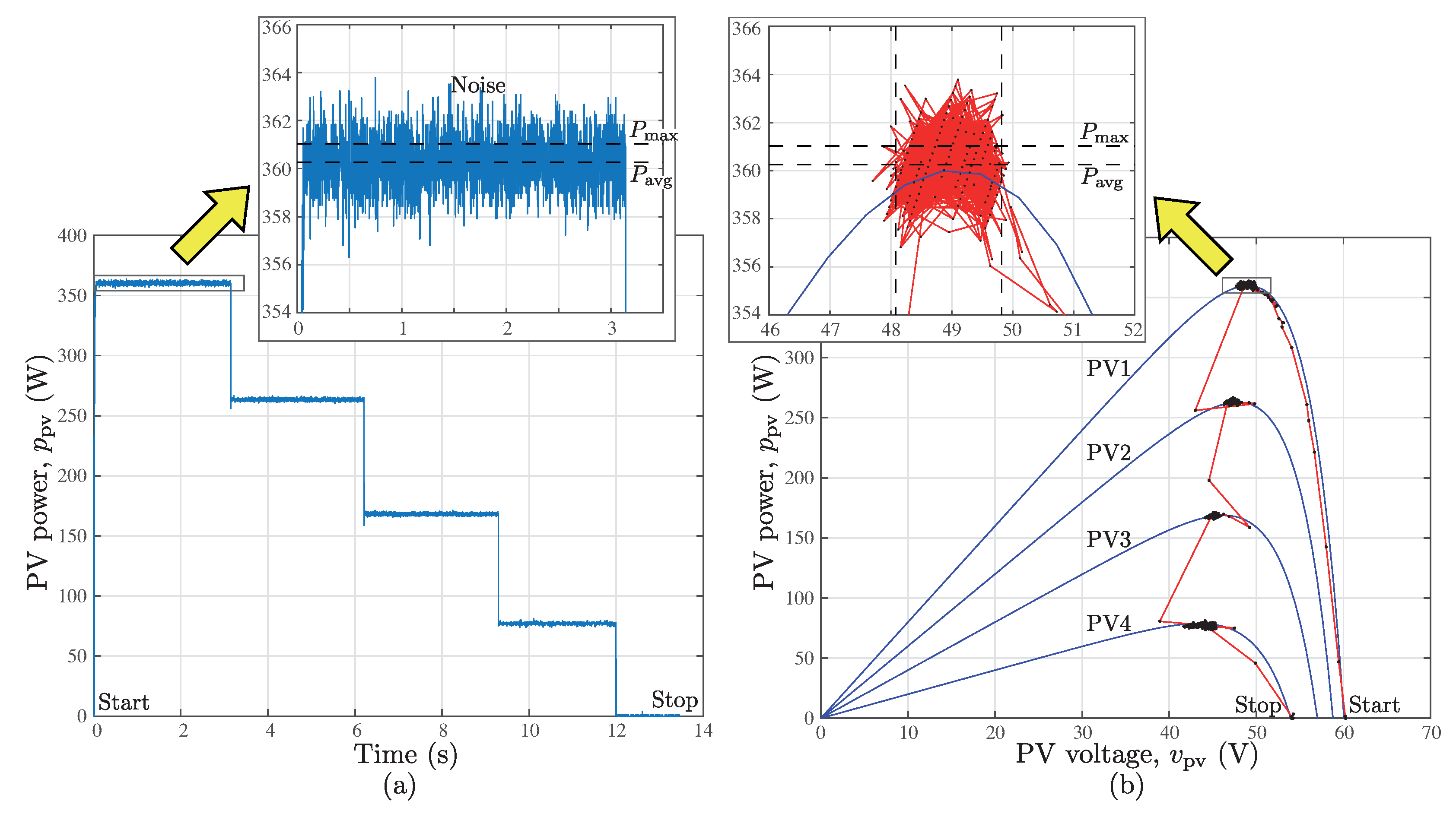
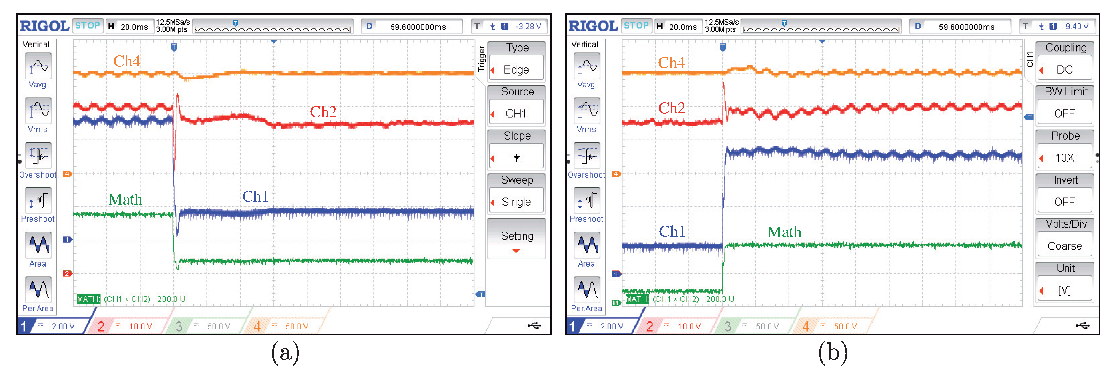
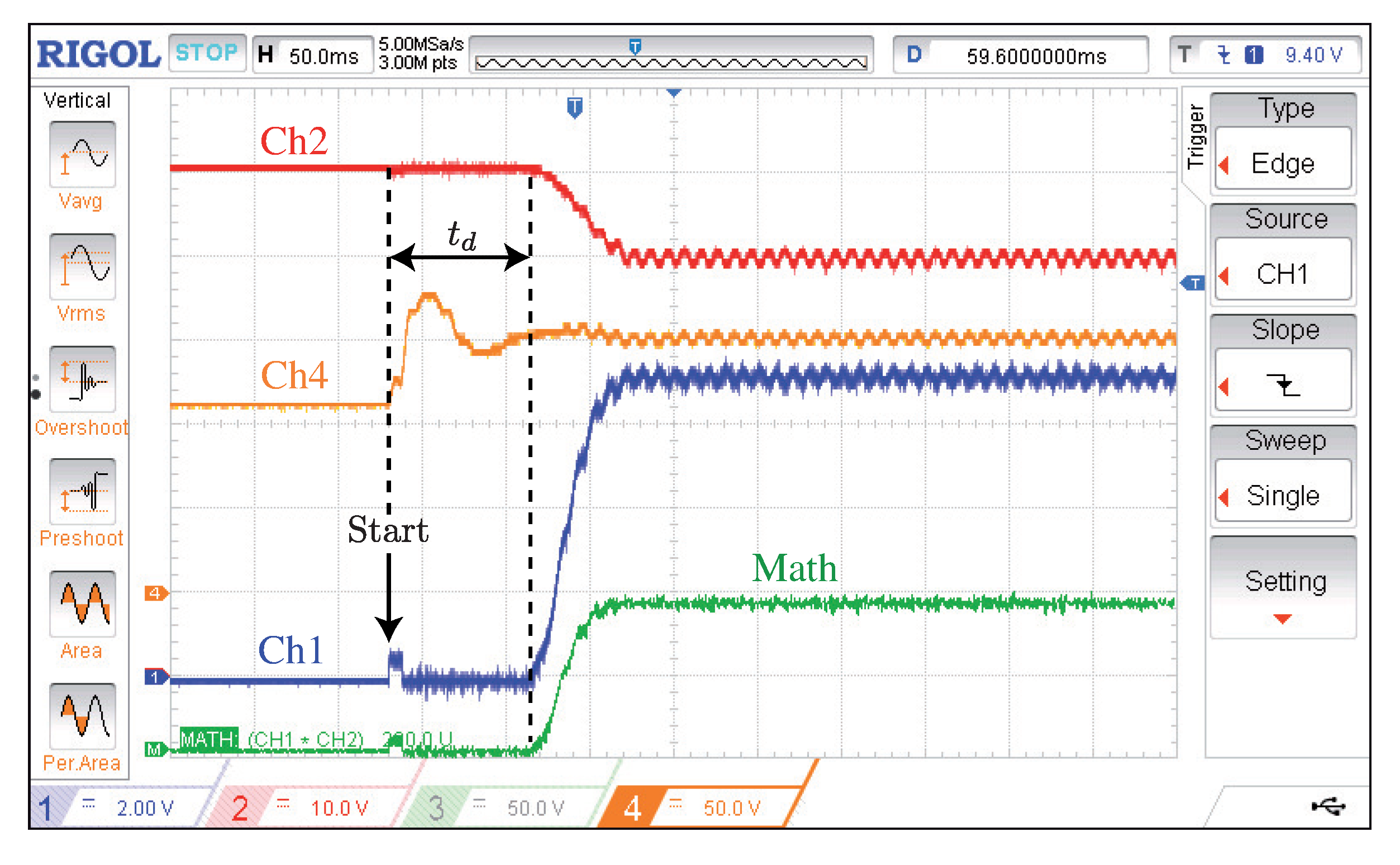
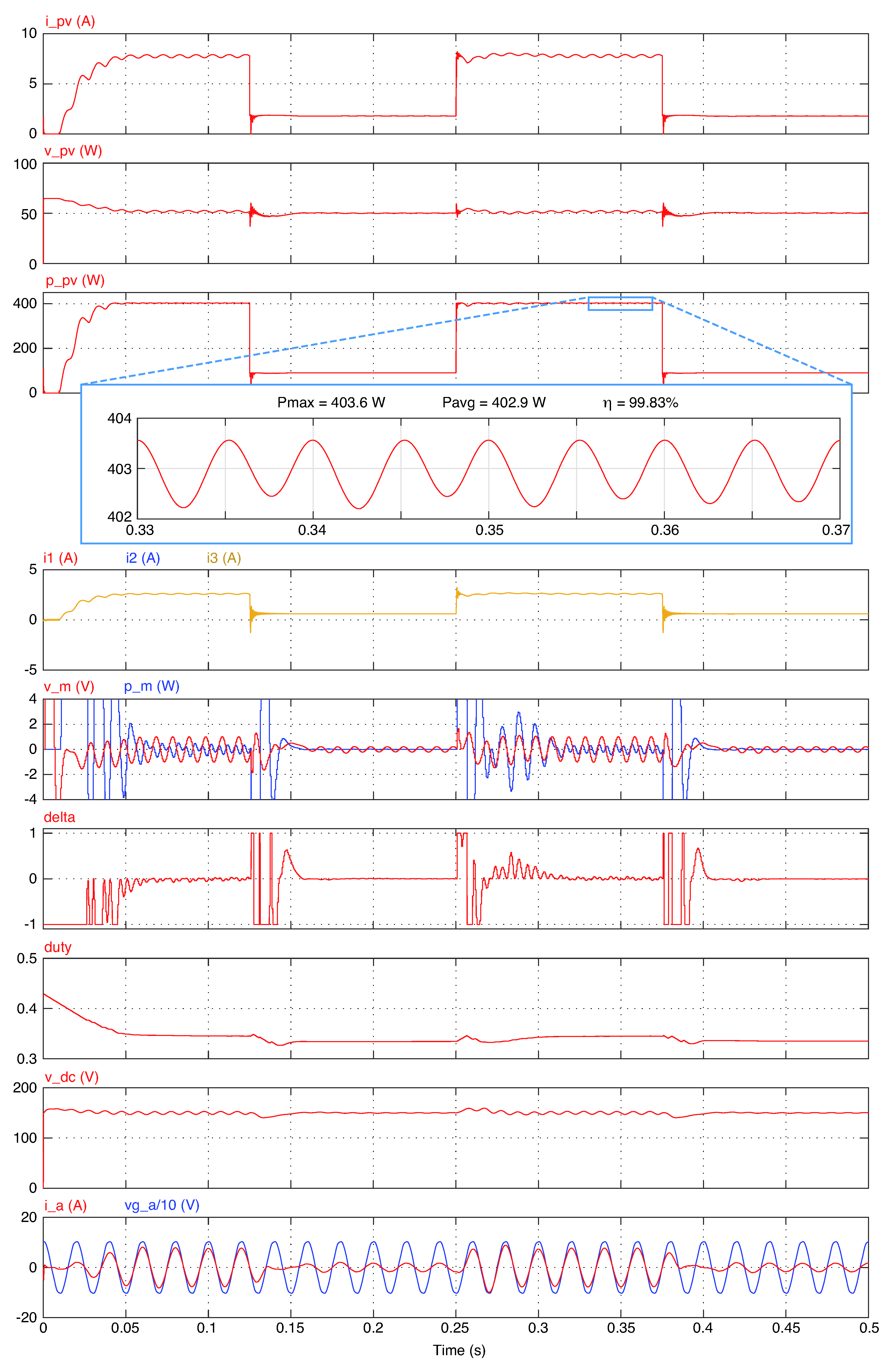
7. Experimental Results

In order to validate the proposed PSD-MPPT, the PV inverter shown in Figure 2 was built with values specified in Table 2. All three boost converters in parallel were implemented using a single IPM-PS22A79 IGBT module from Mitsubishi, where the upper transistors were kept off, and the lower transistors were switched at 10 kHz. Though a commercial inverter for grid connection could have been used, it was also built using another IPM module. The parameters of the inverter were not relevant for the MPPT study and, therefore, are omitted. Fast fuses were added at the input of each boost converter that disconnected them in case of over-current. PV voltage and current were measured using the LV25-P and LTS15-NP sensors, respectively.
The control of the PV converter was resolved in a Renesas RX630 micro-controller at a sampling rate of only 1.82 kHz, using a single PWM output to drive all transistors. The required measurements were only the DC-bus voltage to implement over-voltage and under-voltage protections and the PV voltage and current to implement the MPPT.
All tests shown below were performed using the 480 W E4350B solar array simulator from Agilent. Since the maximum programmable open-circuit voltage was 70 V, a reduced DC-bus voltage of 150 V was set, instead of the standard 400 V, and the grid voltage was also reduced using a transformer with a turn-ratio 1:3.
In order to register the experimental results, the PV converter was communicated with a PC via USB at a transfer speed of 2 kB/s. Data were structured into two channels and two bytes/channel, which resulted in a sampling rate of 500 samples/s for both channels. The USB communication was also used to send power reference values from the PC.
The first test shown in Figure 18 was to produce irradiance level changes in the following sequence: Level 1 (1000 W/m 2 ), Level 2 (750 W/m 2 ), Level 3 (500 W/m 2 ), and Level 4 (250 W/m 2 ). Each irradiance level was maintained for approximately three seconds. The converter turned on at Level 1 and turned off at Level 4. The time-plot of generated power is shown in Figure 18a. Every new MPP was achieved immediately without fluctuations, i.e., without energy loss. A magnified view of the power at maximum irradiance is also shown, obtaining an average power reading P avg = 360.3 W. It is convenient to point out that the measurements shown were not filtered at all, to avoid altering the fast dynamics of this MPPT. As a consequence, the presented measurements contained noise, making it difficult to identify the maximum power P max . This value was obtained in a different experiment, filtering the measurements of the voltage v pv and the current i pv and operating without MPPT, moving the duty-cycle in open-loop. A value of P max = 361.1 W was found. This represents a photovoltaic efficiency η = 100 · 360.3 / 361.1 = 99.77 %.
Figure 18b shows the evolution of the operating point in the P-V curves. Note that the time elapsed between two consecutive points was only 2 ms. The theoretical P-V curves are orientative and differ approximately 1 W from the measurements taken. In the magnified view provided, it can be observed that the movement of v pv was less than 2 V peak-peak around the MPP, which confirms the design of 4% of V MPP = 49 V. According to the theoretical PV curve, these fluctuations would produce power variations that coincide with those calculated above.
In Figure 19, the transient produced by a large step in irradiance is shown in more detail. In Figure 19a, the irradiance is suddenly reduced from 1 kW/m 2 (curve PV1) to 250 W/m 2 (curve PV4), and in Figure 19b, is increased from the PV4 to PV1 curve. The presence of the 100 Hz harmonic can be observed in v pv and i pv measurements, but not in power (Math channel). The MPPT took approximately 60 ms to find the new V MPP .
Figure 20 and Figure 21 are intended to show the ability of the MPPT to track power references. They were obtained under the same conditions as the simulated results presented in Figure 16 and Figure 17, respectively. Specifically, in Figure 20, power reference steps were applied between 200 and 500 W, and in Figure 21, the steps were between 0 and 500 W. The results fully agreed with those of the simulation, showing settling times of less than 70 ms, which corresponded to the worst case of a complete transition from the open-circuit condition to the MPP.
Figure 22 shows the start-up process of the PV inverter. Before the start-up, the DC-bus remained charged to the rectified mains voltage. When the inverter was switched on, it took power from the grid to charge the DC-bus up to 150 V. This turned the array blocking diode off, and the array kept in open-circuit state. During time t d , the MPPT progressively increased the duty-cycle of transistors, decreasing the voltage of the input capacitor until the blocking diode turned on. From here, the MPPT took about 70 ms to reach the MPP.
Finally, Figure 23 shows the effect of a converter activation/deactivation. Figure 23a starts from a situation in which all the power is delivered by one converter. When a second converter is activated, the power is distributed between them after about 60 ms. From this situation, in Figure 23b, the converter is switched off again, and the power is again managed by a single converter in less than 5 ms. It is observed that currents are balanced when both converters are active and that the activation/deactivation does not produce current peaks or alter the operation in the MPP.

8. Conclusions

This article presented a new MPPT method for two stage PV inverters with single phase connection to the power grid. The method takes advantage of the second harmonic of the grid voltage, present in the DC-bus voltage, to guide the MPP search. It consists of detecting the slope of the P-V curve and integrating it to obtain the duty-cycle. The power slope detector (PSD) was able to calculate the slope to command the MPPT even at very low powers, where the amplitude of the oscillations was almost imperceptible. Design equations were provided, both for the gain of the PSD and for the gain of the MPPT integrator.
It was shown how this PSD-MPPT strategy could be combined with the power control, allowing the regulation of powers lower than those of the MPP. The power regulation loop was analyzed and its stability related to a single gain to be designed.
The experimental and simulated results, which fully agreed, demonstrated that the PSD-MPPT method could work without measuring the current in the step-up converter, which implies a cost reduction, especially in the case of parallel arrangement of converters. A PV efficiency of around 99.8% was obtained with a usual ripple in the DC-bus of 4% peak-peak. This result matched the forecasts in Table 1. In addition, the PSD-MPPT method was characterized as being extremely fast, both in the MPP search and in the power regulation, showing response times around 50 ms in the presented results.
Finally, it is worth mentioning that the PSD-MPPT is a simple algorithm of constant parameters that can be solved in a low cost microcontroller at a sampling frequency of only 2 kHz, requiring only the PV voltage and current.

Author Contributions

J.M.E. proposed the main idea, performed the theoretical analysis and wrote the paper, and J.C. contributed to the development and discussion of the results. All authors have contributed to the practical implementation and have performed the experiments. All authors have read and approved the final manuscript.

Funding

This research received no external funding.

Conflicts of Interest

The authors declare no conflict of interest.

References

  1. Sajadian, S.; Ahmadi, R.; Zargarzadeh, H. Extremum Seeking-Based Model Predictive MPPT for Grid-Tied Z-Source Inverter for Photovoltaic Systems. IEEE J. Emerg. Sel. Top. Power Electron. 2019, 7, 1904–1914. [Google Scholar] [CrossRef]
  2. Pahari, O.P.; Subudhi, B. Integral sliding mode-improved adaptive MPPT control scheme for suppressing grid current harmonics for PV system. IET Renew. Power Gener. 2018, 12, 216–227. [Google Scholar] [CrossRef]
  3. Kumar, N.; Hussain, I.; Singh, B.; Panigrahi, B.K. Normal Harmonic Search Algorithm-Based MPPT for Solar PV System and Integrated With Grid Using Reduced Sensor Approach and PNKLMS Algorithm. IEEE Trans. Ind. App. 2018, 54, 6343–6352. [Google Scholar] [CrossRef]
  4. Sangwongwanich, A.; Blaabjerg, F. Mitigation of Interharmonics in PV Systems With Maximum Power Point Tracking Modification. IEEE Trans. Power Electron. 2019, 34, 8279–8282. [Google Scholar] [CrossRef]
  5. Rezk, H.; Aly, M.; Al-Dhaifallah, M.; Shoyama, M. Design and Hardware Implementation of New Adaptive Fuzzy Logic-Based MPPT Control Method for Photovoltaic Applications. IEEE Access 2019, 7, 106427–106438. [Google Scholar] [CrossRef]
  6. Gonzalez-Medina, R.; Liberos, M.; Marzal, S.; Figueres, E.; Garcera, G. A Control Scheme without Sensors at the PV Source for Cost and Size Reduction in Two-Stage Grid Connected Inverters. Energies 2019, 12, 2955. [Google Scholar] [CrossRef]
  7. Chandra Mouli, G.R.; Schijffelen, J.H.; Bauer, P.; Zeman, M. Design and Comparison of a 10-kW Interleaved boost Converter for PV Application Using Si and SiC Devices. IEEE J. Emerg. Sel. Top. Power Electron. 2017, 5, 610–623. [Google Scholar] [CrossRef]
  8. Ho, C.N.; Breuninger, H.; Pettersson, S.; Escobar, G.; Serpa, L.A.; Coccia, A. Practical Design and Implementation Procedure of an Interleaved boost Converter Using SiC Diodes for PV Applications. IEEE Trans. Power Electron. 2012, 27, 2835–2845. [Google Scholar] [CrossRef]
  9. Ahmed, J.; Salam, Z. An Enhanced Adaptive P&O MPPT for Fast and Efficient Tracking Under Varying Environmental Conditions. IEEE Trans. Sustain. Energy 2018, 9, 1487–1496. [Google Scholar]
  10. Ahmed, J.; Salam, Z. A Modified P&O Maximum Power Point Tracking Method With Reduced Steady-State Oscillation and Improved Tracking Efficiency. IEEE Trans. Sustain. Energy 2016, 4, 1506–1515. [Google Scholar]
  11. Macaulay, J.; Zhou, Z. A Fuzzy Logical-Based Variable Step Size P&O MPPT Algorithm for Photovoltaic System. Energies 2018, 11, 1340. [Google Scholar]
  12. Li, C.; Chen, Y.; Zhou, D.; Liu, J.; Zeng, J. A High-Performance Adaptive Incremental Conductance MPPT Algorithm for Photovoltaic Systems. Energies 2016, 9, 288. [Google Scholar] [CrossRef]
  13. Espi, J.M.; Castello, J. A Novel Fast MPPT Strategy for High Efficiency PV Battery Chargers. Energies 2019, 12, 1152. [Google Scholar] [CrossRef]
  14. Galiano, I.; Ordonez, M. PV Energy Harvesting Under Extremely Fast Changing Irradiance: State-Plane Direct MPPT. IEEE Trans. Ind. Electron. 2019, 66, 1852–1861. [Google Scholar]
  15. Paz, F.; Ordonez, M. High-Performance Solar MPPT Using Switching Ripple Identification Based on a Lock-In Amplifier. IEEE Trans. Ind. Electron. 2016, 63, 3595–3604. [Google Scholar] [CrossRef]
  16. Sangwongwanich, A.; Yang, Y.; Blaabjerg, F.; Wang, H. Benchmarking of Constant Power Generation Strategies for Single-Phase Grid-Connected Photovoltaic Systems. IEEE Trans. Ind. App. 2018, 54, 447–457. [Google Scholar] [CrossRef]
Figure 1. PV inverter, where the DC-DC converter is implemented using N interleaved boost converters.
Energies 12 04379 g001
Figure 2. The grid connected PV-inverter prototype built to test the proposed PSD-MPPT method.
Energies 12 04379 g002
Figure 3. Converter model: (a) large-signal averaged model; (b) small-signal model.
Energies 12 04379 g003
Figure 4. Approximated equivalent circuit of the DC-bus: (a) large-signal model; and (b) AC model.
Energies 12 04379 g004
Figure 5. Resulting PV power modulation at different operating points: at the left of the MPP (red, with p ˜ pv and v ˜ pv in phase), at the right of the MPP (green, with p ˜ pv and v ˜ pv in anti-phase), and at the MPP (blue, where p ˜ pv doubles the frequency of v ˜ pv ).
Energies 12 04379 g005
Figure 6. (a) Distortion effect on i pv and (b) its effect on PV efficiency.
Energies 12 04379 g006
Figure 7. Realization of the power slope detector (PSD).
Energies 12 04379 g007
Figure 8. Performance of the band-pass filter G BP ( z ) : (a) frequency response; and (b) step response.
Energies 12 04379 g008
Figure 9. Transients produced by a fast change in power: (a) calculated AC power p m ; (b) slope detector output δ .
Energies 12 04379 g009aEnergies 12 04379 g009b
Figure 10. Proposed MPPT method based on the P-V slope detection.
Energies 12 04379 g010
Figure 11. Simulated results of the proposed MPPT method against irradiance steps between 250 W/m 2 and 1 kW/m 2 . The static efficiency at 1 kW/m 2 is 99.83%.
Energies 12 04379 g011
Figure 12. Proposed modification to achieve PV power control.
Energies 12 04379 g012
Figure 13. Performance of the proposed power control: (a) when the requested power is higher than available PV power; (b) when requested power is lower than available PV power.
Energies 12 04379 g013
Figure 14. Small-signal block diagram of the proposed power control.
Energies 12 04379 g014
Figure 15. Resulting open-loop Bode diagrams when operating at: (a) V pv = V oc with a single active module (worst-case dynamics); and (b) V pv = V MPP with the three modules activated. PM, phase margin; GM, gain margin.
Energies 12 04379 g015
Figure 16. Simulated results at a constant irradiance of 1 kW/m 2 with power reference step changes between 200 W and 500 W.
Energies 12 04379 g016
Figure 17. Simulated results at a constant irradiance of 1 kW/m 2 with power reference step changes between 0 W and 500 W.
Energies 12 04379 g017
Figure 18. Operating point shift during irradiance step changes: (a) time plot of power; and (b) P-V plot. The converter is switched on at PV1, and then, irradiance is changed to PV2, PV3, and PV4. The converter is finally switched off at PV4 (sample time = 2 ms).
Energies 12 04379 g018
Figure 19. Detailed transient responses against irradiance steps: (a) from PV1 to PV4; and (b) from PV4 to PV1. Ch1: PV current (2 A/div). Ch2: PV voltage (10 V/div). Ch4: DC-bus voltage (50 V/div). Math: PV power (200 W/div).
Energies 12 04379 g019
Figure 20. Response against power reference steps between 200 W and 500 W: (a) at the PV module, where Ch1 is the PV current (5 A/div), Ch2 is the PV voltage (10 V/div), CH4 is a power reference synchronism, and Math is the PV power (200 W/div); (b) at the inverter side, where Ch1 is the transformer’s current (5 A/div), Ch2 is the reduced grid voltage (200 V/div), Ch3 is the DC-bus voltage (50 V/div), and CH4 is the power reference synchronism.
Energies 12 04379 g020aEnergies 12 04379 g020b
Figure 21. Response against power reference steps between 0 W and 500 W: (a) at the PV module, where Ch1 is the PV current (5 A/div), Ch2 is the PV voltage (10 V/div), CH4 is a power reference synchronism, and Math is the PV power (200 W/div); (b) at the inverter side, where Ch1 is the transformer’s current (5 A/div), Ch2 is the reduced grid voltage (200 V/div), Ch3 is the DC-bus voltage (50 V/div), and CH4 is the power reference synchronism.
Energies 12 04379 g021
Figure 22. Start-up process of the PV inverter. Ch1: PV current (2 A/div). Ch2: PV voltage (10 V/div). Ch4: DC-bus voltage (50 V/div). Math: PV power (200 W/div).
Energies 12 04379 g022
Figure 23. Activation/deactivation of parallelized converters: (a) turn-on of Converter 2 and current sharing with Converter 1; (b) turn-off of Converter 2 and all power is handled by Converter 1. Ch1: Converter 1 input current (2 A/div). Ch2: Converter 2 input current (2 A/div). Ch3: PV current (2 A/div). Ch4: on/off synchronism.
Energies 12 04379 g023
Table 1. PV Module parameters and attainable efficiencies.
DescriptionVariableValue
Number of PV modules in series n s 3
Number cells/module n c 36
Open-circuit voltage @ 1kW/m 2 V OC 65 V
Short-circuit current @ 1kW/m 2 I SC 8.5 A
Maximum power point voltage @ 1kW/m 2 V MPP 55.5 V
Maximum power point current @ 1kW/m 2 I MPP 7.6 V
Efficiency @ v ˜ dc = 2% peak-peak η | 2 % 99.94%
Efficiency @ v ˜ dc = 4% peak-peak η | 4 % 99.78%
Efficiency @ v ˜ dc = 6% peak-peak η | 6 % 99.44%
Efficiency @ v ˜ dc = 8% peak-peak η | 8 % 99.09%
Efficiency @ v ˜ dc = 10% peak-peak η | 10 % 98.50%
Table 2. PV converter parameters.
DescriptionVariableValue
Number of boost convertersN3
Nominal powerP450 W
Switching frequency f s w 10 kHz
DC-bus voltage V dc 150 V
DC-bus capacitance C dc 1470 μ F
Input filter inductances L j 1200 μ H
Inductor series resistances r j 25 m Ω
Input capacitanceC470 μ F
Table 3. PSD-MPPT control parameters.
DescriptionVariableValue
Sampling frequency f s = 1 T 20/11 kHz
Slope detector’s gain k m 2500
Bandpass filters, center-frequency f 0 100 Hz
Bandpass filters, bandwidth f BW 100 Hz
Integrator’s gain k i 2 rad/s
Power gain (power control) k p 0.01
Minimum PV current for start-up i min 50 mA

