Robust Design Optimization of Electromagnetic Actuators for Renewable Energy Systems Considering the Manufacturing Cost

Abstract

Power transmission and protection of power electronics–electromagnetic actuators are crucial parts in renewable energy systems (energy management of photovoltaic, wind power, hybrid and electric vehicles). Consistency optimization of electromagnetic actuators has attracted extensive attention from corporations in competitive markets. Robust design has been widely applied for reducing the influence of uncertainties in the manufacturing process to improve the consistency of product quality. However, the cost factors of the actual manufacturing process are not fully considered in state-of-art methods. Although the consistency has been improved, the optimization scheme may not be optimal from the perspective of engineering applications, because unnecessary cost increments may be produced. In this paper, an application-oriented robust design method for consistency optimization is proposed. The impact of tolerance values on quality loss and manufacturing cost can be considered simultaneously to guide the tolerance optimization process. Thus, the optimal solution of total loss is obtained by optimizing the quality fluctuation to the design objective with the minimum increment of manufacturing cost. An example of the consistency optimization of an electromagnetic actuator used in the photovoltaic system is presented to illustrate the procedure and verify the effectiveness of the proposed method.

1. Introduction

Fossil energies such as oil, natural gas and coal are among the world’s main energy sources, which account for most of the global primary energy consumption. Due to the non-renewability of fossil energy and a series of environmental pollution problems caused by its use, it is imperative to find reliable alternative energy sources and green energy consumption methods [1]. Energy sources such as wind, hydro and solar energy can be recycled rapidly and used as a viable alternative to fossil energy [2]. With the continuous deepening of renewable energy generation and power consumption in recent years, the reliability requirements for related products are also increasing. Among them, the quality fluctuation of electronic components and energy storage devices has become the main cause of renewable energy system failures [3]. Most of the current research has focused on the conversion and storage of renewable energy sources [4,5,6]. However, the optimization of robust and consistency of electronic components is rarely mentioned.

Electromagnetic actuators play a crucial role of circuit conversion, automatic adjustment, safety protection and are used extensively in renewable energy systems such as photovoltaic power generation, wind power generation and charging piles for electric vehicles, as shown in Figure 1. However, the complex structure and manufacturing process of the electromagnetic actuators are important reasons for their poor consistency and reliability [7]. The uncertainties in the production process will inevitably deviate the output response from the design values to affect the consistency and reliability of the batch product [8,9], especially for the electromagnetic actuators containing a great many technique processes during the manufacture.

At present, actuator manufacturers mainly rely on screening to control the consistency of external performances, such as operating voltage, operating time, etc., while ignoring the internal characteristics such as holding force, contact pressure for the product consistency. As Figure 2 shows, although the same number of qualified products can be obtained through screening and quality consistency design, the reliability is quite different. Both methods have 1000 qualified samples within the L_L~U_L threshold, but the inherent reliability is 0.9972 for quality consistency design, while the inherent reliability of screening is only 0.8664.

In the manufacturing process of batch products, the quality loss occurs when the quality characteristic value is out the customer’s tolerance limits [10]. Meanwhile, the manufacturing cost is necessary to ensure that the manufacturing capacity is in the producer’s tolerance limits [11]. It is obvious that the smaller of the quality loss, the higher of the manufacturing costs. Therefore, Taguchi [12] defined the total loss as the sum of quality loss and manufacturing cost and indicated that the reduction of quality loss should be more than the increase of manufacturing cost for the optimization scheme [13]. The robust tolerance design method was proposed based on orthogonal experimental design to describe the significance of each tolerance to the consistency for tolerance allocation [14].

The robust design method has been proven to be suitable for non-linear and explicit/implicit functions in many fields [15]. For instance, Lee et al. [16] used the Taguchi method to optimize the electromotive force of interior permanent magnet synchronous motor to enhance the product quality. Gao et al. [17] adopted the Taguchi robust design to improve the absorption efficiency of an electromagnetic wave absorber by tightening the performance variation level. In the field of robust design for electromagnetic actuators, Liang et al. [18] combined the reliability design with robust design in the electromagnetic system of actuators to obtain an effective solution. Zhai et al. [19] optimized the cooperation between electromagnetic force and spring force of electromagnetic actuator by robust design method to improve the consistency of product output.

The fundamental theories of Taguchi’s method are widely recognized [20,21]. Although it can improve the robustness, its optimization results may not be the optimal solution [22]. Sometimes, its optimization accuracy cannot be guaranteed in practical applications [23]. In previous research of robust design for electromagnetic actuators, there has been a drawback in state-of-art methods that the impact of manufacturing costs is not considered in the robust optimization process [24], and the changes of manufacturing cost and total loss are calculated only after the optimization [25]. Although consistency has been improved, it may result in a huge increase in manufacturing cost in practical applications.

The manufacturing costs can commonly be defined as the sum of fixed costs and variable costs [26]. The massive production usually has high fixed costs and low variable costs by establishing precision automation production line, but for the small batch production like electromagnetic actuators, the variable costs are much higher than the fixed costs with a lot of manual work. The reduction of tolerances will inevitably lead to the increase of manufacturing costs. Therefore, the contribution rate should not be the only factor for optimization and the increase of manufacturing costs must be considered at the same time. Only in this way can the optimal solution of total loss be obtained by optimizing the quality fluctuation to the design objective with the minimum increment of manufacturing cost.

Considering both quality loss and manufacturing cost, there is some research focusing on the improvement of experimental techniques [27]. Jeang [28] proposed a tolerance chart balancing method to minimize the total cost of manufacturing and designing activities in the early stages of a machining process. Terán et al. [29] established a present worth model to express the quality loss during service, so the quality loss during a certain service life can be transformed to the present worth on the time node before the product leaves the factory. Then, Zhao et al. [30] proposed the service quality loss model based on the present worth model to reduce the total loss by prolonging the product service life. Khodaygan [31] optimized the tolerances of mechanical assemblies with degrading components to find the best asymmetric tolerances from Pareto solutions by combining Shannon’s entropy-based TOPSIS algorithm with robust design.

However, the above references are methods to reduce the total loss at the current quality loss level. The objective of optimizing consistency to specified requirements has not been explicitly proposed, which is essential for the actuator to improve the product quality and avoid the waste of cost.

Aiming at improving consistency and reducing total loss, an application-oriented robust design method is proposed in this paper. The cost contribution rate is established referring to the form of fluctuation contribution rate in Taguchi’s method. Then, the optimal solution of total loss satisfying the consistency optimization objective can be obtained by using the two contribution rates together in the robust optimization process.

The paper is organized as follows: In Section 2, the models of robust design optimization are presented in details. Section 3 gives the procedure of optimization. Section 4 illustrates the effectiveness of the proposed method via the robust optimization of an electromagnetic actuator. Finally, conclusions are given in Section 5.

2. Models of Robust Design Optimization

2.1. Average Total Loss Model

In Taguchi’s robust method, total loss T_L is the sum of quality loss L_Q and manufacturing cost C_M. Taguchi indicates that the quality loss will occur if the output response does not reach the optimal design value, even if the product is within the qualified threshold [32].

Assume y is the output response, m is the optimal design value, X = {x₁, …, x_n} are input variables, Τ = {t₁, …, t_n} are tolerance values of input variables, so the quality loss L(y) is defined as [33]

$$L(y)=k{(y-m)}^2$$

(1)

where k is the coefficient calculated by the qualified threshold ±Δ_q and the economic loss of unqualified product A, expressed as

$$A=k{\mathsf{\Delta }}_q^2$$

(2)

Then, the average quality loss L_Q of batch product containing N samples can be expressed as

$$L_Q=\frac{1}{N}{\displaystyle \sum _{p=1}^{N}L(y_p)}=k\frac{1}{N}{\displaystyle \sum _{p=1}^N{(y_p-m)}^2}=\frac{A}{{\mathsf{\Delta }}_q^2}{\sigma }^2$$

(3)

where σ is the standard deviation of output response distribution, which is determined by the input tolerances T. Setting Δ_q = 3σ_q based on the 6σ management, σ_q is the standard deviation of consistency optimization objective. Then, the average quality loss L_Q is a function of input tolerances Τ, which may be written as

$$L_Q=\frac{A}{9}{\left(\frac{\sigma (T)}{{\sigma }_q}\right)}^2$$

(4)

The manufacturing costs are related to both production volume and input tolerances. However, to be comparable with the average quality loss L_Q, the average manufacturing cost C_M, which is independent of production volume and only related to input tolerances Τ, is proposed in this paper.

To establish the mathematical expression of the relationship between cost and tolerance, it is necessary to establish a uniform model based on the actual process data. Wu et al. [34] presented five functions; namely, reciprocal, reciprocal squared, Sutherland–Roth, exponential and Michael–Siddall. In this paper, the reciprocal function is employed to build the establish the functional relationship between manufacturing cost C_i and tolerance t_i, expressed as

$$C_i(t_i)={\alpha }_{i1}+\frac{{\alpha }_{i2}}{t_i+{\alpha }_{i3}}$$

(5)

where α_i1~α_i3 are constant coefficients, which are determined by converting the actual manufacturing cost corresponding to tolerance t_i to a single product.

So, the average manufacturing cost C_M can be written as

$$C_M={\displaystyle \sum _{i=1}^n{C}_i\left(t_i\right)}$$

(6)

It should be noted that the manufacturing cost model chosen in this paper can be modified or replaced arbitrarily in practical applications, without affecting the process and precision of robust optimization.

Based on the above models, the average total loss T_L can be established as

$$T_L=\frac{A}{9}{\left(\frac{\sigma (T)}{{\sigma }_q}\right)}^2+{\displaystyle \sum _{i=1}^n{C}_i\left(t_i\right)}$$

(7)

which is related to the input tolerances Τ = {t₁, …, t_n}.

2.2. Fluctuation Contribution Rate Model

Defining the total quality loss of output response is L_Q when each input variable x_i fluctuates within its tolerance range t_i, then, the fluctuation contribution rate ρ_i is defined to quantify the effect of tolerance t_i on the total quality loss L_Q, which is the percentage of the quality loss L_i caused by input tolerance t_i in the total quality loss L_Q and may be expressed as [35]

$${\rho }_i(t_i)=\frac{L_i(t_i)}{L_Q}$$

(8)

Because of that

$$L_Q={\displaystyle \sum _{i=1}^n{L}_i(t_i)}+e$$

(9)

where e represents the noise or error observed in the response y, the sum of fluctuation contribution rates of all input variables is 100%, written as

$${\displaystyle \sum _{i=1}^n{\rho }_i(t_i)}+{\rho }_e=100\%$$

(10)

where ρ_e is fluctuation contribution rate of error.

In Taguchi’s robust tolerance design method, the orthogonal experimental design and variance analysis are adopted to analyze the fluctuation contribution rates for all the input variables. By using the most commonly used three-levels orthogonal design, where level 2 is the central value x_i of input variable, level 1 and level 3 are the lower limit value x_i − t_i and the upper limit value x_i + t_i, the contribution rate ρ_i of tolerance t_i is calculated by

$${\rho }_i(t_i)={\rho }_{il}(t_i)+{\rho }_{iq}(t_i)$$

(11)

where ρ_il and ρ_iq are the monomial contribution rate and quadratic contribution rate of the tolerance t_i because the degree of freedom of three-levels is 2. They can be estimated by

$${\rho }_{il}(t_i)=\frac{{(T_{1i}-T_{3i})}^2-2r{V}_e}{2r{S}_T}$$

(12)

$${\rho }_{iq}(t_i)=\frac{{(T_{1i}-2T_{2i}+T_{3i})}^2-6r{V}_e}{6r{S}_T}$$

(13)

where S_T is the sum of the total deviation square of the results of output response y in the orthogonal table. V_e is the error variance. T_1i, T_2i and T_3i are the sub-sum of the experiment results y corresponding to 3 levels of x_i. r is repetition number of the same level in the orthogonal table.

According to the above equations, if tolerances of arbitrary inputs change, the fluctuation contribution rates of all inputs will be affected. Therefore, the results of fluctuation contribution rate need to be updated with the change of tolerance values in the robust optimization process, to reflect correctly the influence of tolerances on fluctuation and ensure the optimization accuracy. Meanwhile, the reduction of tolerance should be determined according to the fluctuation contribution rate in the robust optimization process. Tolerances with a high fluctuation contribution rate have great influence on quality fluctuation, so a large reduction should be set up.

2.3. Cost Contribution Rate Model

With the decrease of tolerance values, the increase of cost must be considered at the same time. Therefore, the amount of tolerance reduction should be appropriately decreased if the tolerance is sensitive to cost.

In this paper, the cost contribution rate ξ_i is proposed referring to the form of fluctuation contribution rate ρ_i; to quantify the effect of tolerance t_i on the total manufacturing cost C_M. So, it can be defined as the percentage of the cost increment ΔC_i caused by tolerance reduction Δt_i in the total cost increment ΔC_M caused by all the tolerance reductions, which may be expressed as

$${\xi }_i(t_i)=\frac{\mathsf{\Delta }{C}_i}{\mathsf{\Delta }{C}_M}=\frac{C_i(t_i+\mathsf{\Delta }{t}_i)-C_i(t_i)}{{\displaystyle \sum _{i=1}^n\left[C_i(t_i+\mathsf{\Delta }{t}_i)-C_i(t_i)\right]}}$$

(14)

In each iteration, the reduction amount of all the tolerances is very small and can be considered as Δt₁ = … = Δt_n. So, the above equation can be converted to

$${\xi }_i(t_i)=\frac{{\kappa }_i\cdot \mathsf{\Delta }{t}_i}{{\displaystyle \sum _{i=1}^n{\kappa }_i\cdot \mathsf{\Delta }{t}_i}}=\frac{{\kappa }_i(t_i)}{{\displaystyle \sum _{i=1}^n{\kappa }_i(t_i)}}$$

(15)

where κ_i is the slope of the manufacturing cost function C_i at the tolerance value t_i written as

$${\kappa }_i(t_i)={\frac{\mathrm{d}{C}_i}{\mathrm{d}{t}_i}|}_{t_i}$$

(16)

Like fluctuation contribution rate model, the cost contribution rate model has

$${\displaystyle \sum _{i=1}^n{\xi }_i(t_i)}=100\%$$

(17)

The cost contribution rates of all inputs will also be affected if tolerances of arbitrary inputs change. Therefore, the results need to be updated with the change of tolerance values in the robust optimization process. Meanwhile, tolerances with a high cost contribution rate have great influence on manufacturing cost, so the reduction amount should be decreased.

2.4. Robust Optimization Model

In our previous studies, the tolerances with large contribution rates to output fluctuation are preferred to reduce in the tolerance optimization, so that the consistency can be improved with the minimum tolerance changes. However, ignoring the impact of cost in this process does not necessarily lead to the best optimization scheme with minimum total loss if the costs of significant tolerances are very high. Therefore, the purpose of cost calculation in this paper is to avoid using tolerances with high impact but high cost, and to encourage the use of tolerances with low cost and certain impact. In this way, the same consistency optimization result can be achieved with less cost. To determine the tolerance reductions in consideration of impact and cost, the robust optimization model is established combining the two contribution rates defined above, which may be expressed as

$$\mathsf{\Delta }{t}_i=\frac{{\rho }_i}{{\xi }_i}\delta$$

(18)

where δ is coefficient, which can be determined according to the size of input tolerance values and the requirements of iteration times.

Because there is a limit to the improvement of manufacturing capability, the amount of tolerance reduction Δt_i should be set to 0 when the tolerance value t_i has reached the lower limit γ_i. So, the robust optimization model for the iterative optimization process can be established as

$$\mathsf{\Delta }{t}_{i(j+1)}=\{\begin{array}{l}\frac{{\rho }_i}{{\xi }_i}\delta \left(t_{i(j)}>{\gamma }_i\right)\\ 0\left(t_{i(j)}\le {\gamma }_i\right)\end{array}$$

(19)

where j is the iteration number.

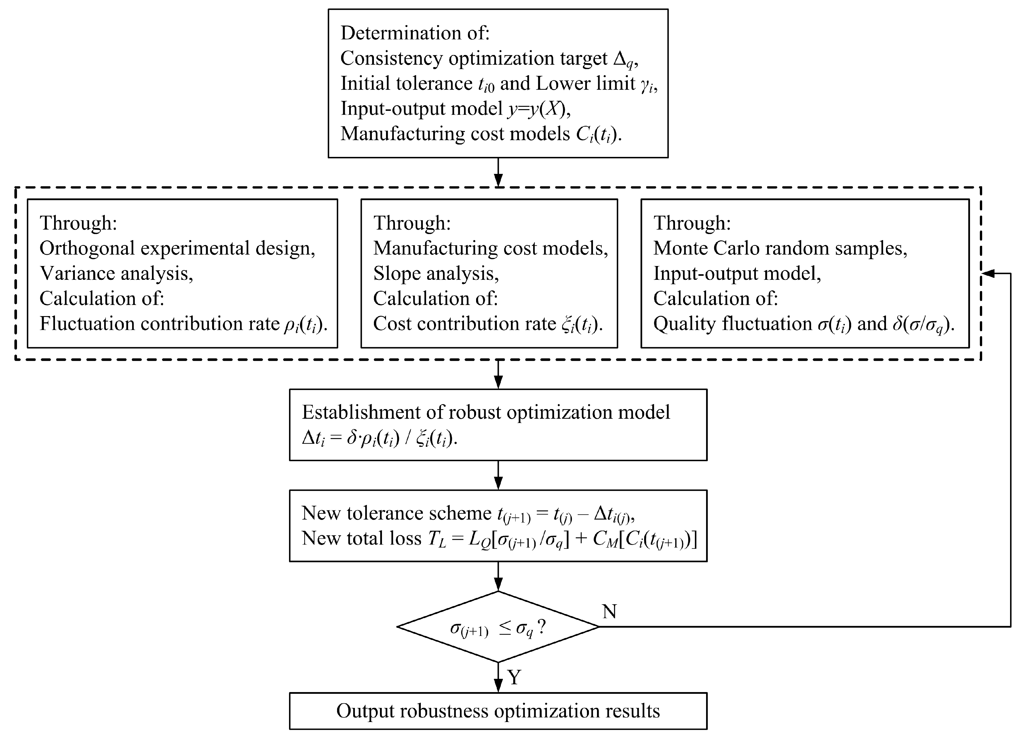
3. Procedure of Robust Design Optimization

The procedure of robust design optimization proposed in the paper is shown in Figure 3.

First, the qualified threshold Δ_q is chosen as the consistency optimization target. Also, the initial tolerance value t_i0 and the lower limit γ_i of each input variable x_i are needed. The calculation model between input variables and output response could be established by a simulation method or approximate modeling method. Then, the output distribution of the initial tolerance scheme can be obtained by the Monte Carlo simulation technique to calculate the initial standard deviation σ₀ and quality loss L_Q0. Meanwhile, the initial manufacturing cost C_M0 can be calculated according to the manufacturing cost models. So, the initial total loss T_L0 can be obtained.

Second, the fluctuation contribution rates ρ_i are calculated through the orthogonal experimental design and variance analysis, and the cost contribution rate ξ_i are calculated according to the slope analysis results. Then, the robust optimization model Δt_i can be established combining the coefficient δ.

Third, the new tolerance scheme T_{(j + 1)} in the (j + 1)^th iteration is determined based on the amount of tolerance reduction Δt_i(j). Then, the new total loss T_{L(j + 1)} and quality fluctuation σ_{(j + 1)} can be obtained.

In each iteration, the impact of tolerance values on both quality loss and manufacturing cost can be simultaneously considered by the tolerance optimization model to guide the tolerance optimization process. Meanwhile, the three coefficients in the tolerance optimization model can be updated with the variation of tolerance values. In this way, the tolerances with the highest cost performance can be selected to reduce in each iteration, to determine the new tolerance scheme. Consequently, the consistency can gradually approximate the optimization objective with the minimum manufacturing cost.

4. Case Study

The high-power DC contactor is a typically electromagnetic actuator widely used in photovoltaic systems. Its structure is described in Figure 4 and includes electromagnetic system, armature moving system and reaction system. The armature system is the movable mechanism to implement the working process of pickup and release. The electromagnetic system is basically made of magnetic material, which consists of shell, iron core, yoke, armature and coil. When the coil is carrying the rated current, magnetic flux will be generated in the magnetic circuit. Then, the electromagnetic attraction force will be formed on the armature, to drive it from the release position to the pickup position. During this process, the reaction system, which is composed of touch bridge, link, reaction spring, rebound spring and static contacts, produces reaction forces. For example, the contact between touch bridge and static contacts will generate contact pressures, meanwhile the springs are compressed to form spring forces. When the armature system is at the pickup position, the retention force is the difference between electromagnetic attraction force and reaction forces. In addition, the operating voltage and time of the pickup process are called the operating characteristics.

The vibration resistance and electrical life are two main performance indexes of electromagnetic actuator. First of all, the retention force directly determines the vibration resistance of the electromagnetic actuator and affects the reliability of the energy system under extreme application environment.

Secondly, the retention force affects the contact depth of the contact, and then, it affects the reliability and consistency of the contact resistance, which has great influence on one of the heat sources of the electromagnetic actuator. The excessive heating will seriously affect the efficient and reliable operation of the energy system.

Finally, the retention force will influence the operating characteristics of the electromagnetic actuator, which will affect its working efficiency in the protection of new energy system. The slow operating speed will even endanger the safety of the whole system and operators.

Therefore, in this paper, the retention force is critical to product reliability and is selected as the objective function of robust design optimization. The eleven input variables are chosen for the robust design optimization. Their tolerance values and lower limits are determined according to the actual manufacturing process, as

Table 1. Tolerances and lower limits of input variables.

Input Variables	Initial Tolerances	Lower Limits
A—Yoke assembly position (mm)	±0.5	±0.05
B—Armature assembly position (mm)	±0.5	±0.05
C—Yoke polar diameter (mm)	±0.4	±0.05
D—Armature polar diameter (mm)	±0.2	±0.05
E—Armature outer diameter (mm)	±0.2	±0.05
F—Core diameter (mm)	±0.2	±0.05
G—Iron core outer diameter (mm)	±0.25	±0.05
H—Coil resistance/10* (Ω)	±0.4	±0.05
I—Reaction spring preload/2* (N)	±0.5	±0.05
J—Rebound spring preload/2* (N)	±0.5	±0.05
K—Contact pressure/2* (N)	±0.5	±0.05

*Note: The values are divided to make the tolerances in the same order of magnitude to other variables.

shows.

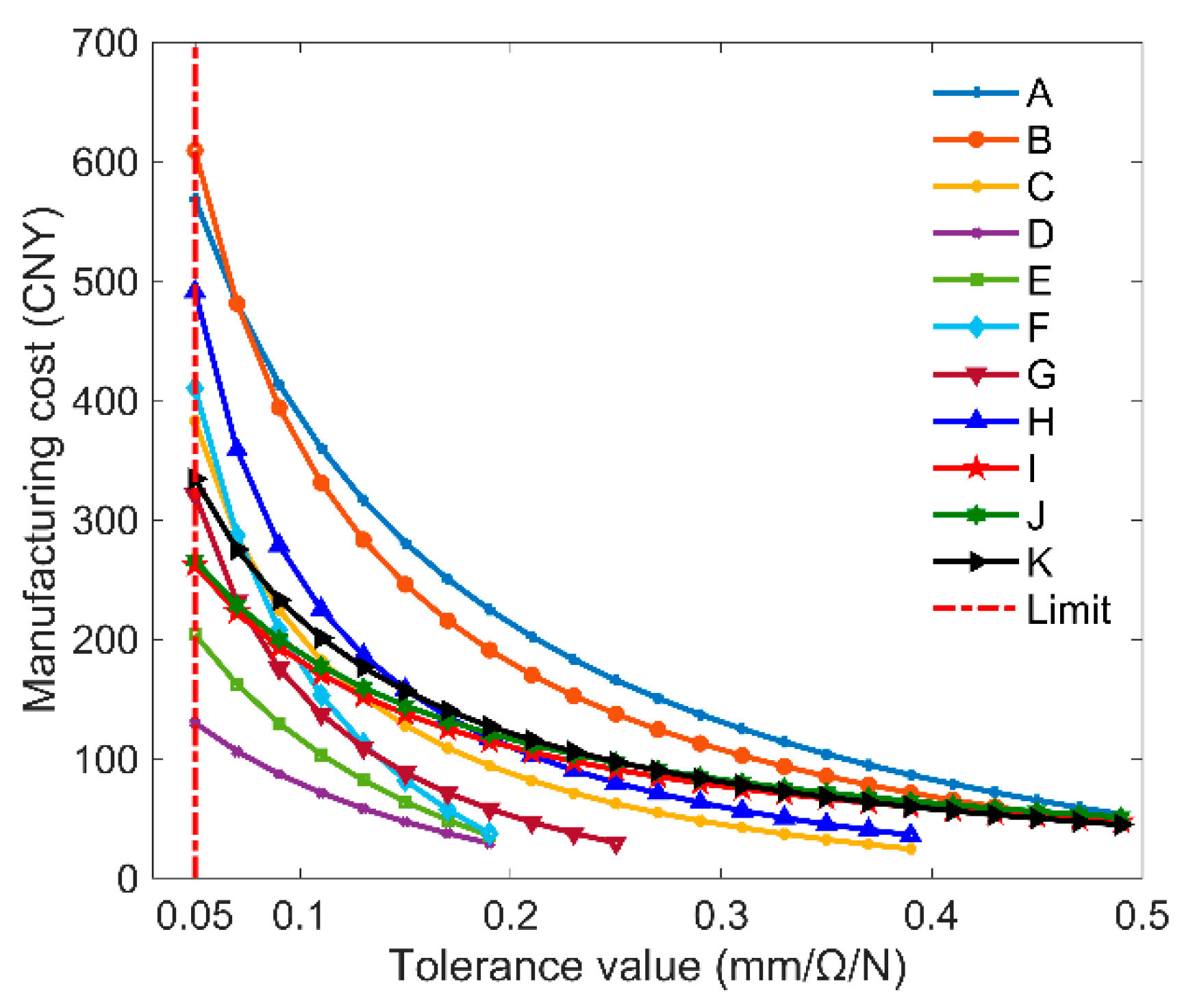
4.1. Manufacturing Cost Models

The manufacturing cost models of input variables are established based on the process data collected in the actual production. There are two situations. If the variable is realized by machining, such as factors C, D, E, F and G, the cost of unqualified products will increase when the tolerance is reduced. If the variable is achieved by manual work, for example, the factors A, B, H, I, J and K, the working hours will increase when the tolerance is reduced. In brief, the manufacturing cost will increase nonlinearly with the decrease of tolerance, as shown in Figure 5. By using the uniform model of Equation (5), the manufacturing cost models can be obtained, where the coefficients are shown in

Table 2. Coefficients of manufacturing cost models.

Coefficients	αi1	αi2	αi3	Ci0 (CNY)
A	–102.13	89.20	0.083	50.87
B	–63.00	57.13	0.035	43.79
C	–48.20	29.73	0.019	22.76
D	–88.73	35.87	0.114	25.49
E	–137.73	49.20	0.094	29.61
F	–151.40	39.87	0.021	28.99
G	–68.00	26.07	0.017	29.63
H	–45.53	32.73	0.011	34.11
I	–10.87	32.47	0.069	46.19
J	–11.47	35.53	0.078	50.01
K	–21.00	35.53	0.050	43.61

.

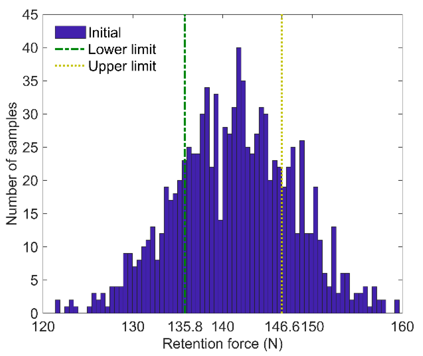
4.2. Initial Total Lost

The calculation model between input variables and retention force of contactor is established by the Kriging method. Setting the number of samples to 1000, the virtual samples of batch product are generated by the Monte Carlo method. So, the output distribution of the initial tolerance scheme can be obtained and is shown in Figure 6. Its mean value is 141.2 N and standard deviation σ₀ is 6.57 N.

Setting the qualified threshold of consistency optimization to be 135.8–146.6 N, the optimization objective σ_q is calculated to be 1.8 N. The economic loss of unqualified product A is 1200 determined by the actual production of contactor. So, the initial quality loss L_Q0 is calculated to be 1777.2 according to Equation (4). The initial manufacturing cost C_M0 is calculated to be 405.1 by using Equations (5) and (6). Then, the initial total lost T_L0 can be calculated to be 2182.3 by using Equation (7).

4.3. Robust Optimization Model

Taking the first iterative process as an example, the tolerance of each variable is the initial value T₀. According to the fluctuation contribution rate model and the cost contribution rate model, the contribution rates of each variable are calculated separately. The results are shown in

Table 3. Results of contribution rates in the first iteration.

Input Variables	ρi (%)	ξi (%)	Δti
A	13.52	8.04	0.0818
B	32.16	6.12	0.2557
C	2.21	5.18	0.0208
D	3.94	11.14	0.0172
E	2.48	17.44	0.0069
F	0.93	25.01	0.0018
G	0.87	11.20	0.0038
H	14.48	5.94	0.1186
I	11.65	3.07	0.1847
J	11.10	3.26	0.1657
K	6.44	3.60	0.0871

.

By using Equation (18), the robust optimization model can be established, where δ is determined according to the size of input tolerance values and the requirements of iteration times. To automatically adjust the tolerance reduction according to the extent of the output fluctuation range approaching the qualified threshold so that both the convergence speed and optimization accuracy are guaranteed, the coefficient δ is defined as

$$\delta =0.001\times {\left(\frac{\sigma (T)}{{\sigma }_q}\right)}^h$$

(20)

Setting the value of h to 3, the tolerance reduction of each variable in the first iteration can be calculated and is shown in Table 3. Then, the quality loss L_Q1, manufacturing cost C_M1 and total loss T_L1 can be obtained according to the new tolerance scheme T₁. By repeating the above steps, the tolerance optimization process can be obtained and the results are shown in Figure 7.

Meanwhile, the conventional method, which refers to the robust design method proposed by Taguchi, is utilized to do the same robust design optimization. In this method, the tolerance reductions are only determined by the fluctuation contribution rates. Then, the increase of manufacturing cost and change of total loss are calculated after tolerance optimization. The results of the conventional method are also shown in Figure 7.

It can be seen from the comparison results that the quality loss L_Q with the two methods are both reduced accurately to the consistency optimization objective. However, the increment of manufacturing cost ΔC_M of conventional method is 33% higher than that of proposed method. Finally, the change of total loss ΔT_L is −166 obtained by the proposed method, which indicates that the reduction of quality loss is greater than the increase in manufacturing cost. It is a good solution according to Taguchi’s theory. Meanwhile, the change of total loss ΔT_L is 323 obtained by the conventional method, which does not meet the ideal requirements in robust design.

In the initial stage of tolerance optimization, the speed of quality loss reduction is faster than that of manufacturing cost increase. So, the total loss T_L shows a rapid downward trend. However, with the decrease of tolerance values, the non-linear cost-increase relationships in Figure 7 make the manufacturing cost increase rapidly, leading to a change in the trend of total loss. Therefore, it is easy to find an effective solution for singly reducing the total loss according to the above rules, but to add a specific requirement for consistency on this basis, the optimization scheme may not be ideal if simply using the influence of tolerance on quality fluctuations and ignoring the impact of manufacturing cost.

Furthermore, the influence of the constant h in Equation (19) of δ on the optimization process is studied. As Figure 8a,b shows, when h increases from 1 to 3, the number of iterations is shortened from 113 to 42 times, but the optimization result of total loss T_L only changes 0.4%. The dotted gray lines in Figure 8a,b are the datum lines with h = 1. When h is increased to 3.5, the optimization results are obviously wrong. Therefore, the best value of h is determined as 3.

4.4. Consistency Optimization Results

Figure 9 shows the variation of fluctuation contribution rates during the robust optimization process. Figure 10 shows the change in the cost contribution rates. Under the joint influence of these two factors, the tolerance values of variables are determined and shown in Figure 11 and

Table 4. Tolerance values of variables before and after robust design optimization.

Input Variables	Initial Values	Optimal Values	Normalized Values
A—Yoke assembly position (mm)	±0.5	±0.150	±0.15
B—Armature assembly position (mm)	±0.5	±0.094	±0.09
C—Yoke polar diameter (mm)	±0.4	±0.166	±0.17
D—Armature polar diameter (mm)	±0.2	±0.058	±0.06
E—Armature outer diameter (mm)	±0.2	±0.091	±0.09
F—Core diameter (mm)	±0.2	±0.145	±0.15
G—Iron core outer diameter (mm)	±0.25	±0.160	±0.16
H—Coil resistance/10* (Ω)	±0.4	±0.098	±0.10
I—Reaction spring preload/2* (N)	±0.5	±0.103	±0.10
J—Rebound spring preload/2* (N)	±0.5	±0.105	±0.11
K—Contact pressure/2* (N)	±0.5	±0.137	±0.14

*Note: The values are divided to make the tolerances in the same order of magnitude to other variables.

. The optimal tolerance values are standardized to meet the labelling requirements in the manufacturing process.

Figure 12 is the change process of the contribution rates and cost increment of factor B with the proposed method. Due to the rapid increase of cost contribution rate, the downward trend of fluctuation contribution rate is limited effectively, thereby reducing the decrease of tolerance value. Its cost increment ΔC_B is 317.1 after optimization. Figure 12b shows the change process of factor B with the conventional method. Since the impact of cost is not considered, its fluctuation contribution rate continues to decrease. The tolerance value is reduced to the lower limit of 0.05 mm at the 40th iteration. Therefore, its cost increment reached a maximum of 571.1, which is 254 (80%) more than the former.

Figure 13a is the change process of factor I with the proposed method. Its tolerance reduction amount is increased because the cost contribution rate is low, to reduce the quality loss with less increment of cost ΔC_I. Compared with the results of conventional method in Figure 13b, the cost is only increased by 13.8 (11%).

The distribution of retention force after robust optimization is shown in Figure 14. Its standard deviation is 1.7949, with an error of 0.3% to the optimization target. Taking the qualified threshold of 135.8–146.6 N, the inherent reliability of the contactor after the optimization can be increased from 0.5889 to 0.9973, thereby greatly improving the application reliability of the product in the renewable energy system.

Finally,

Table 5. Comparison of results before and after robust optimization.

Method	Initial	Conventional	Proposed
Standard deviation	6.57	1.79	1.79
Quality loss	1777.2	132.0	132.6
Manufacturing cost	405.1	2373.1	1883.5
Total loss	2182.3	2505.1	2016.1
Inherent reliability	0.5889	0.9973	0.9973

lists the changes in consistency and total loss before and after the robust design. By comparing the optimization results of the conventional Taguchi method and proposed method, it can be concluded that the proposed method can obtain the better solution with lower cost.

5. Conclusions

As crucial devices with high transmission energy and high isolation depth, electromagnetic actuators are used extensively in renewable energy systems. The consistency of batch products directly affects the inherent reliability and application reliability of electromagnetic actuators, thereby affecting the reliability and safety of renewable energy systems. To overcome the limitation in state-of-the-art methods that the optimization scheme may not be optimal from the perspective of engineering applications, an application-oriented robust design method is proposed to obtain the optimal solution of total loss by optimizing the quality fluctuation to the design objective with the minimum increment of manufacturing cost. The results are as follows:

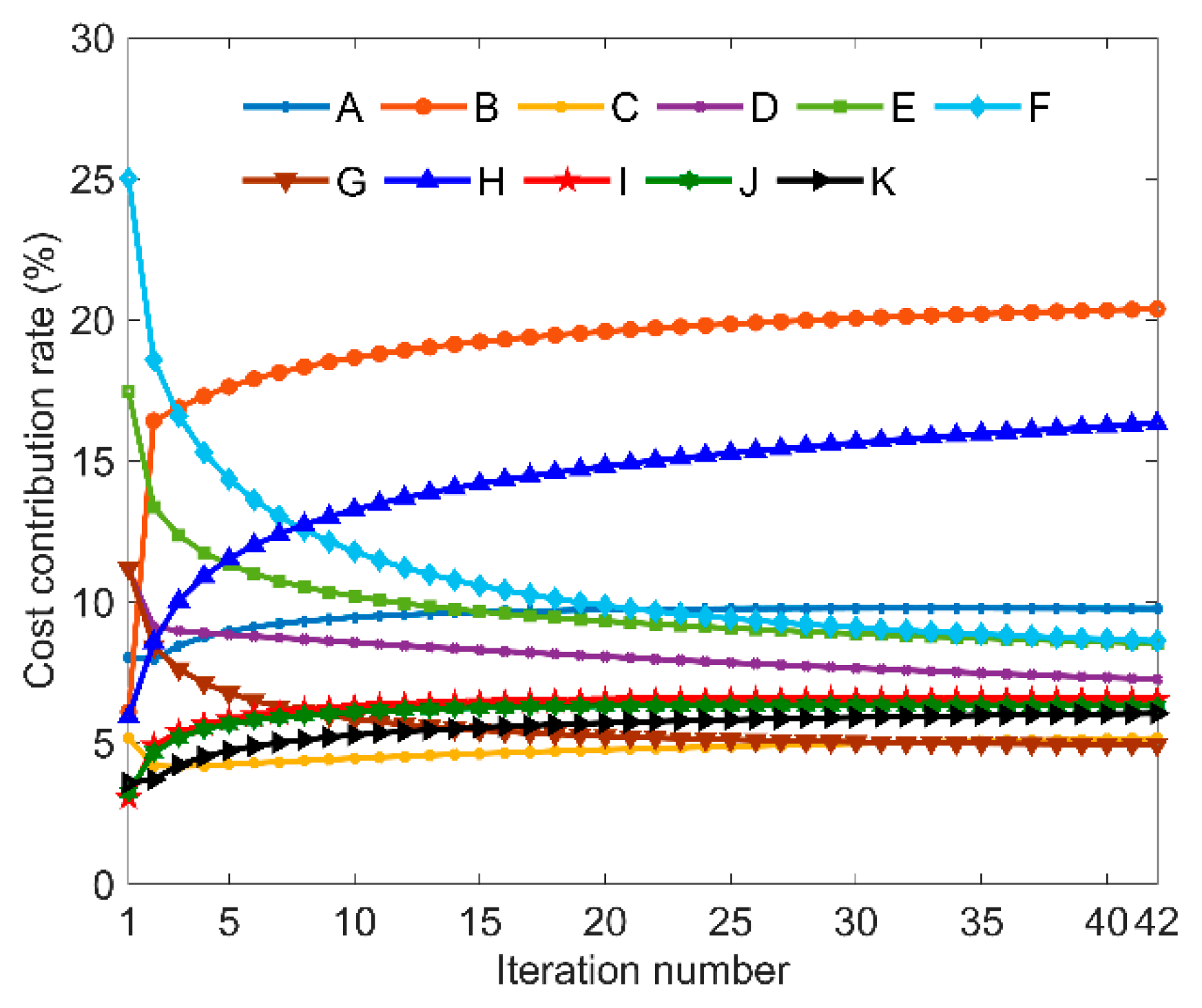
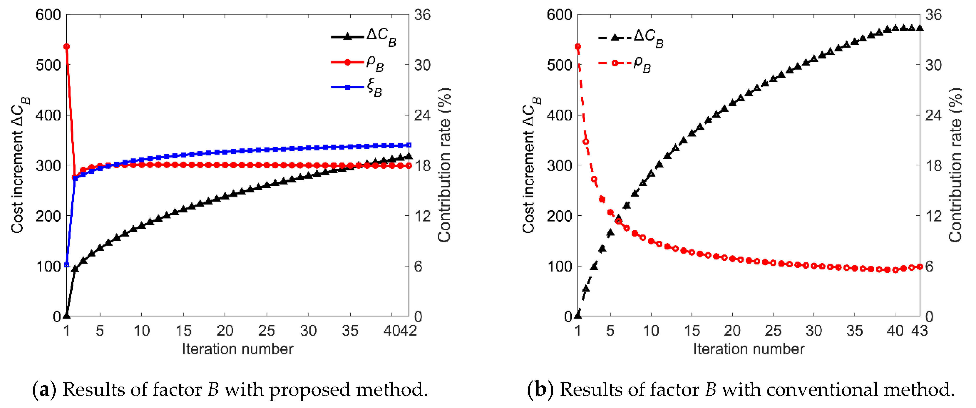
• By using the established robust optimization model combining fluctuation contribution rate and cost contribution rate, the impact of tolerance values on quality loss and manufacturing cost can be considered simultaneously to guide the tolerance optimization process. The downward trend of fluctuation contribution rate of factor B is limited effectively by its rapid increase of cost contribution rate, so the cost increment of this factor has been reduced by 254 (80%). Meanwhile, the cost of factor C is only increased by 13.8 (11%) to reduce the quality loss.
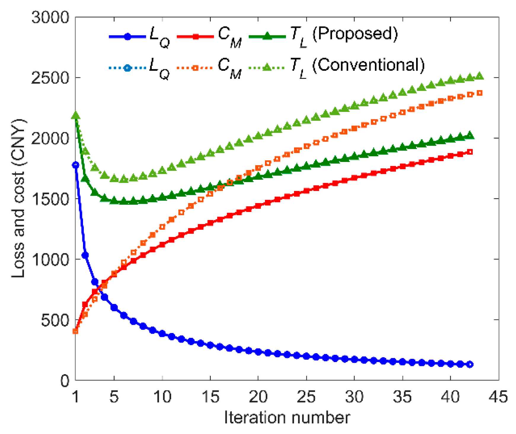
• It is easy to find an effective solution for singly reducing the total loss, but it is a complicated optimization problem to reduce the total loss while improving the consistency to achieve the optimization objective. Through the novel optimization procedure for robust design, the quality loss L_Q is reduced accurately to the optimization target, while the increment of manufacturing cost ΔC_M is 33% less than that of conventional method.
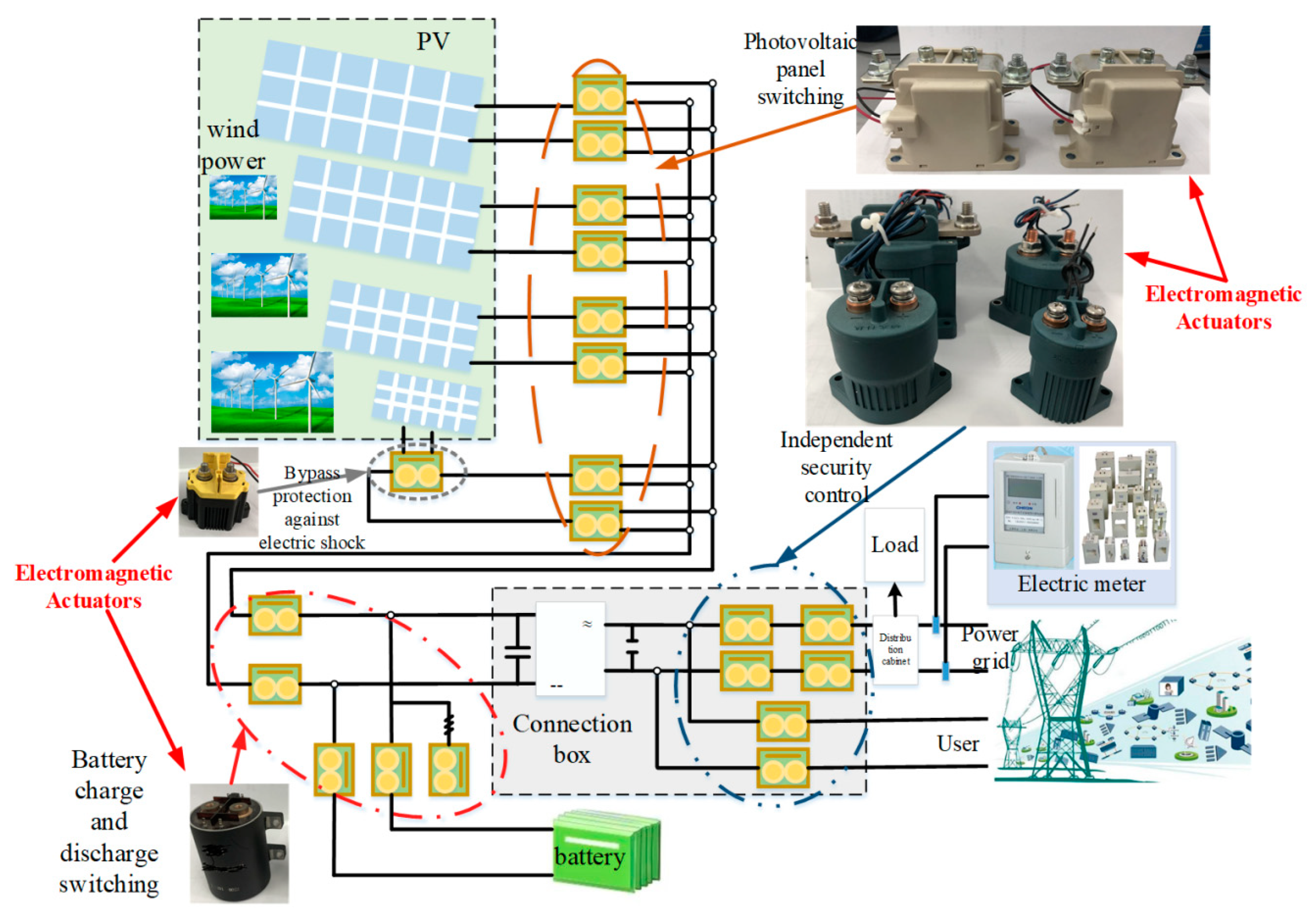
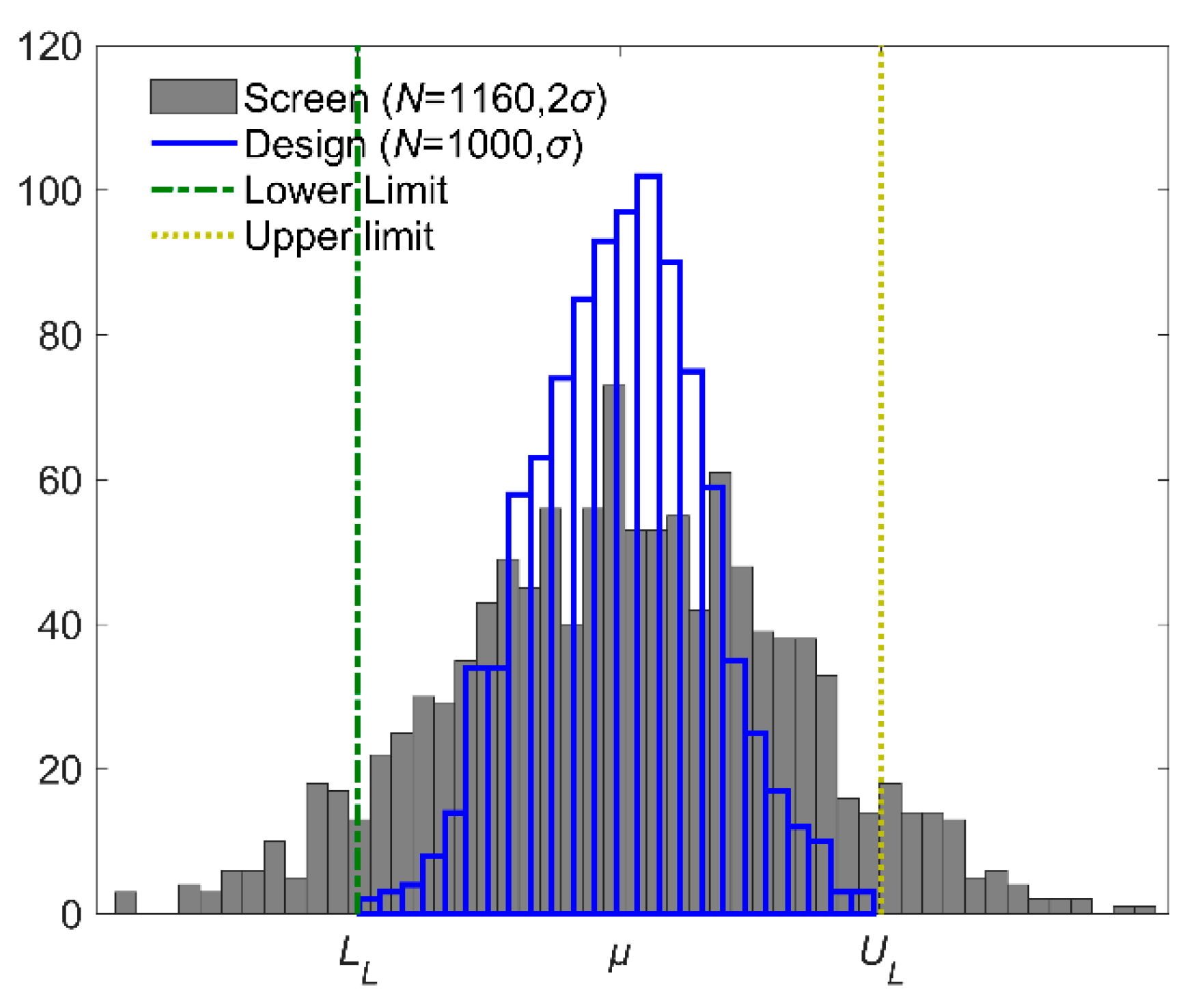
• After the robust design with proposed method, the error of consistency optimization is 0.3%, and the inherent reliability of contactor is increased from 0.5889 to 0.9973(increased by 69.35%), thereby greatly improving the application reliability of the product in the renewable energy system.
• The method proposed in this paper is based on experimental design, and the input–output relationship model is not necessary, so it is universal for non-linear and high-order explicit/implicit functions in many fields. It should be noted that the form of robust optimization model and its coefficient are all based on experience. Meanwhile, when establishing the manufacturing cost models, a unified model is adopted for all the factors to simplify the optimization process. The above assumption and simplification may affect the efficiency and accuracy when applying this method to other optimization problems, but the error can be reduced through further research and improved according to practical applications.

References

1. Astaneh, M.; Roshandel, R.; Dufo-Lopez, R.; Bernal-Agustin, J.L. A novel framework for optimization of size and control strategy of lithium-ion battery based off-grid renewable energy systems. Energy Convers. Manag. 2018, 175, 99–111. [Google Scholar] [CrossRef]
2. Liu, K.; Li, K.; Ma, H.; Zhang, J.; Peng, Q. Multi-objective optimization of charging patterns for lithium-ion battery management. Energy Convers. Manag. 2018, 159, 151–162. [Google Scholar] [CrossRef]
3. Chen, K.D.; Zhao, F.Q.; Hao, H.; Liu, Z.W. Synergistic impacts of China’s subsidy policy and new energy vehicle credit regulation on the technological development of battery electric vehicles. Energies 2018, 11, 3193. [Google Scholar] [CrossRef]
4. Yao, J.W.; Zhang, Y.M.; Yan, Z.; Li, L. A group approach of smart hybrid poles with renewable energy, street lighting and EV charging based on DC micro-grid. Energies 2018, 11, 3445. [Google Scholar] [CrossRef]
5. Da Luz, C.M.A.; Tofoli, F.L.; Vicente, P.D.S.; Vicente, E.M. Assessment of the ideality factor on the performance of photovoltaic modules. Energy Convers. Manag. 2018, 167, 63–69. [Google Scholar] [CrossRef]
6. Merchaoui, M.; Sakly, A.; Mimouni, M.F. Particle swarm optimisation with adaptive mutation strategy for photovoltaic solar cell/module parameter extraction. Energy Convers. Manag. 2018, 175, 151–163. [Google Scholar] [CrossRef]
7. Schuëller, G.I.; Jensen, H.A. Computational methods in optimization considering uncertainties—An overview. Comput. Methods Appl. Mech. Energy 2008, 198, 2–13. [Google Scholar] [CrossRef]
8. Tang, L.C.; Goh, T.N.; Lam, S.W.; Zhang, C.W. Fortification of six sigma: Expanding the DMAIC toolset. Qual. Reliab. Eng. Int. 2007, 23, 3–18. [Google Scholar] [CrossRef]
9. Nilsen, T.; Aven, T. Models and model uncertainty in the context of risk analysis. Reliab. Eng. Syst. Saf. 2003, 79, 309–317. [Google Scholar] [CrossRef]
10. Pedersen, S.N.; Christensen, M.E.; Howard, T.J. Robust design requirements specification: A quantitative method for requirements development using quality loss functions. J. Eng. Des. 2016, 27, 544–567. [Google Scholar] [CrossRef]
11. Liu, M.Z.; Liu, C.H.; Xing, L.L.; Mei, F.D.; Zhang, X. Study on a tolerance grading allocation method under uncertainty and quality oriented for remanufactured parts. Int. J. Adv. Manuf. Technol. 2016, 87, 1265–1272. [Google Scholar] [CrossRef]
12. Taguchi, G. Quality engineering in Japan. Bull. Jpn. Soc. Precis. Eng. 1985, 19, 237–242. [Google Scholar] [CrossRef]
13. Sfantsikopoulos, M.M. A cost-tolerance analytical approach for design and manufacturing. Int. J. Adv. Manuf. Technol. 1990, 5, 126–134. [Google Scholar] [CrossRef]
14. Liang, H.M.; Ren, W.B.; Ye, X.R.; Zhai, G.F. Research on the reliability tolerance analysis method of electromagnetic relay in aerospace. Chin. J. Aeronaut. 2005, 18, 65–71. [Google Scholar] [CrossRef]
15. Cao, Y.; Liu, T.; Yang, J. A comprehensive review of tolerance analysis models. Int. J. Adv. Manuf. Technol. 2018, 97, 3055–3085. [Google Scholar] [CrossRef]
16. Lee, S.; Kim, K.; Cho, S.; Jang, J.; Lee, T.; Hong, J. Optimal design of interior permanent magnet synchronous motor considering the manufacturing tolerances using Taguchi robust design. IET Electr. Power Appl. 2014, 8, 23–28. [Google Scholar] [CrossRef]
17. Gao, R.X.K.; Hoefer, W.J.R.; Li, E.P. Quality synthesis based robust optimization for electromagnetic wave absorbers using Taguchi’s tolerance design method. IEEE Trans. Antenn. Propag. 2014, 62, 2102–2108. [Google Scholar] [CrossRef]
18. Liang, H.M.; Ye, X.R.; Zhai, G.F. Research on the tolerance distribution of sealed electromagnetic relay with reliability index. IEICE Trans. Electron. 2006, E89-C, 1164–1172. [Google Scholar] [CrossRef]
19. Zhai, G.F.; Liang, H.M.; Xu, F.; Liu, M.K. New method of tolerance design of electromagnetic relay reliability. J. Eng. Des. 2004, 15, 425–431. [Google Scholar]
20. Shi, J.; Zhong, Z.; Zhu, X. Robust design and optimization for autonomous PV-wind hybrid power systems. J. Zhejiang Univ. Sci. A 2008, 9, 401–409. [Google Scholar] [CrossRef]
21. Wang, Y.; Li, L.; Hartman, N.W.; Sutherland, J.W. Allocation of assembly tolerances to minimize costs. Cirp. Ann. Manuf. Technol. 2019, 68, 13–16. [Google Scholar] [CrossRef]
22. Tsai, J.T. Robust optimal-parameter design approach for tolerance design problems. Eng. Optim. 2010, 42, 1079–1093. [Google Scholar] [CrossRef]
23. Douglas, C.M. Stu Hunter’s contributions to experimental design and quality engineering. Qual. Eng. 2014, 26, 5–15. [Google Scholar]
24. Deng, J.; Yu, H.D.; Ye, X.R.; Zhai, G.F. Consistency optimization for batch product of electromagnetic relay with improved robust tolerance design method. In Proceedings of the 1st International Conference on Reliability Systems Engineering, Beijing, China, 21–23 October 2015. [Google Scholar]
25. Tang, L.C.; Xu, K. A unified approach for dual response surface optimization. J. Qual. Technol. 2002, 34, 437–447. [Google Scholar] [CrossRef]
26. Ma, B.; Lei, G.; Zhu, J.G.; Guo, Y.G.; Liu, C.C. Application-oriented robust design optimization method for batch production of permanent-magnet motors. IEEE Trans. Ind. Electron. 2018, 65, 1728–1739. [Google Scholar] [CrossRef]
27. Ma, B.; Lei, G.; Liu, C.C.; Zhu, J.G.; Guo, Y.G. Robust tolerance design optimization of a PM claw pole motor with soft magnetic composite cores. IEEE Trans. Magn. 2018, 54, 8102404. [Google Scholar] [CrossRef]
28. Jeang, A. Tolerance chart balancing with a complete inspection plan taking account of manufacturing and quality costs. Int. J. Adv. Manuf. Technol. 2011, 55, 675–687. [Google Scholar] [CrossRef]
29. Terán, A.; Pratt, D.B.; Case, K.E. Present worth of external quality losses for symmetric nominal-is-better quality characteristics. Eng. Econ. 1996, 42, 39–52. [Google Scholar] [CrossRef]
30. Zhao, Y.M.; Liu, D.S.; Wen, Z.J.; Liu, T. Modeling present worth of product quality loss of SIB characteristic based on service life distribution. Appl. Mech. Mater. 2013, 397, 846–851. [Google Scholar] [CrossRef]
31. Khodaygan, S. A multiple objective framework for optimal asymmetric tolerance synthesis of mechanical assemblies with degrading components. Int. J. Adv. Manuf. Technol. 2019, 100, 2177–2205. [Google Scholar] [CrossRef]
32. Robles, N.; Roy, U. Optimal tolerance allocation and process-sequence selection incorporating manufacturing capacities and quality issues. J. Manuf. Syst. 2004, 23, 127–133. [Google Scholar] [CrossRef]
33. Cheng, B.W.; Maghsoodloo, S. Optimization of mechanical assembly tolerances by incorporating Taguchi’s quality loss function. J. Manuf. Syst. 1995, 14, 264–276. [Google Scholar] [CrossRef]
34. Wu, Z.; Elmaraghy, W.H.; Elmaraghy, H.A. Evaluation of cost tolerance algorithms for design tolerance analysis and synthesis. Manuf. Rev. 1988, 1, 168–179. [Google Scholar]
35. Deng, J.; Ye, X.R.; Lin, Y.G.; Li, Q.Y.; Zhai, G.F. A new robust tolerance design method for electromechanical device based on variable contribution rate coefficients. J. Eng. Des. 2017, 28, 532–548. [Google Scholar] [CrossRef]
Figure 1. Application of electromagnetic actuators in renewable energy system.
Energies 12 04353 g001
Figure 2. Quality distributions by screening and consistency design.
Energies 12 04353 g002
Figure 3. Procedure of robust design optimization.
Energies 12 04353 g003
Figure 4. Structure of high-power DC contactor.
Energies 12 04353 g004
Figure 5. Manufacturing cost models of input variables.
Energies 12 04353 g005
Figure 6. Initial output distribution.
Energies 12 04353 g006
Figure 7. Results of tolerance optimization process.
Energies 12 04353 g007
Figure 8. Influences of h on the optimization process.
Energies 12 04353 g008
Figure 9. Variation of fluctuation contribution rates.
Energies 12 04353 g009
Figure 10. Variation of cost contribution rates.
Energies 12 04353 g010
Figure 11. Variation of tolerance values.
Energies 12 04353 g011
Figure 12. Results of factor B with proposed and conventional method.
Energies 12 04353 g012
Figure 13. Results of factor I with proposed and conventional method.
Energies 12 04353 g013
Figure 14. The distribution of retention force after robust optimization.
Energies 12 04353 g014