The Application of Water Cycle Optimization Algorithm for Optimal Placement of Wind Turbines in Wind Farms


Abstract
:
1. Introduction
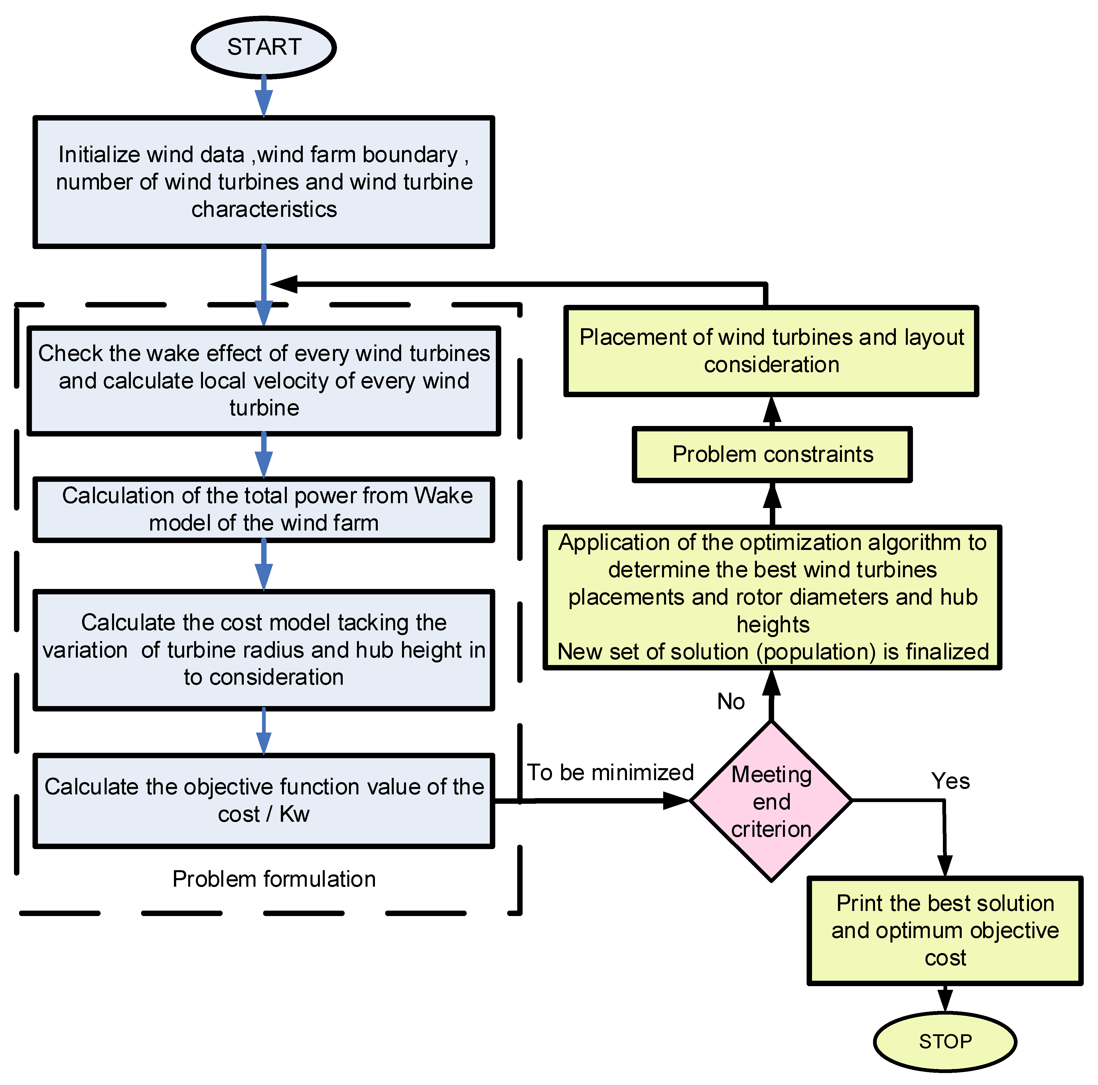
2. Problem Formulation
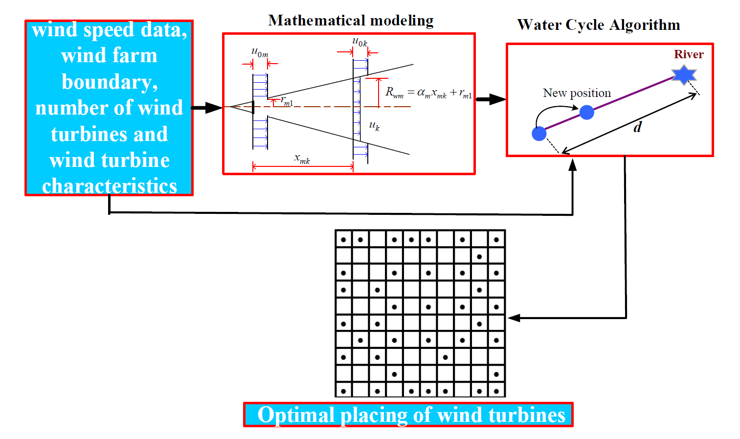
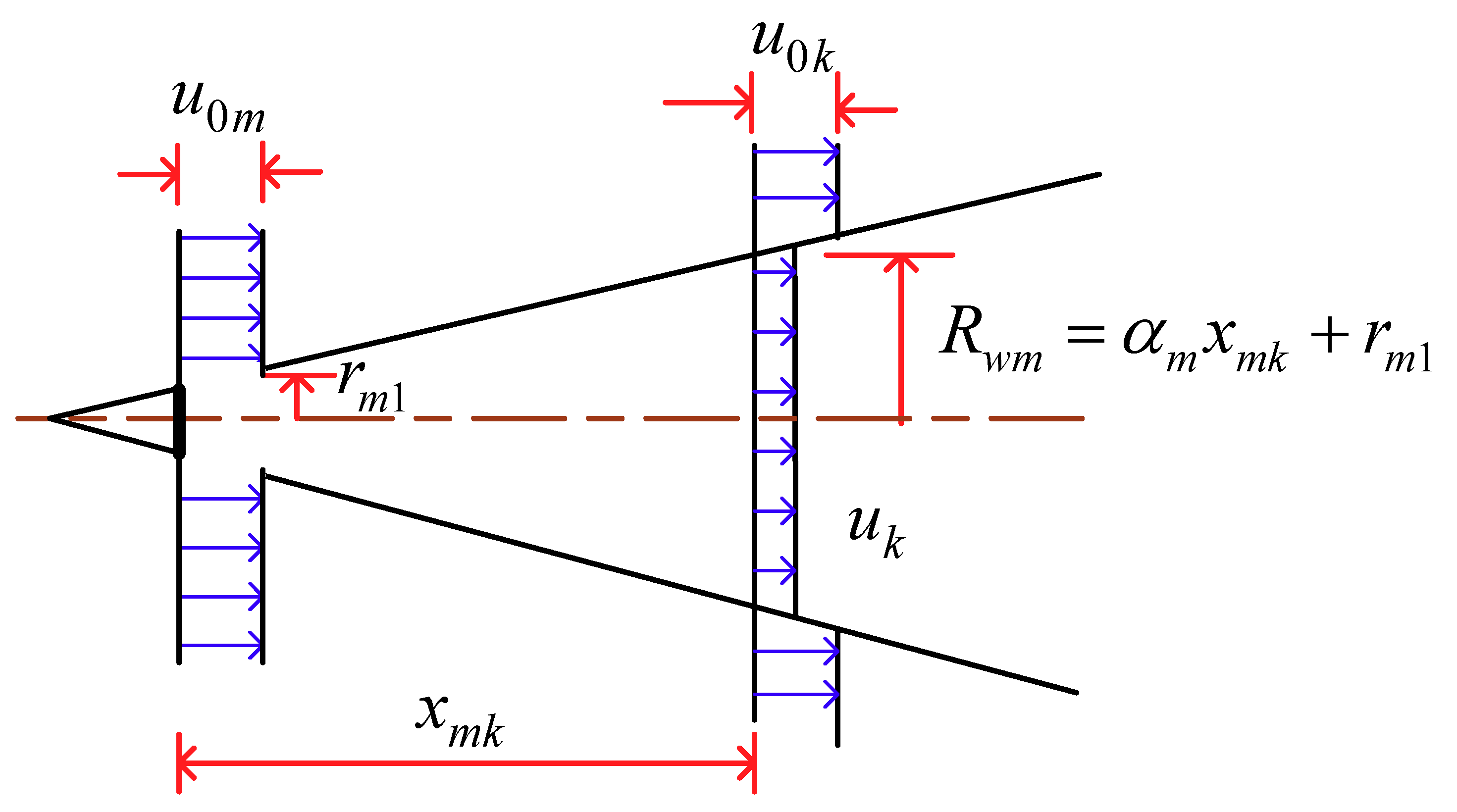
2.1. Wake Model
2.2. Harvested Power Model
2.3. WF Efficiency Model
2.4. Normalized Cost Model
2.5. Objective Function
3. Brief Overview of Modern Optimization Algorithms
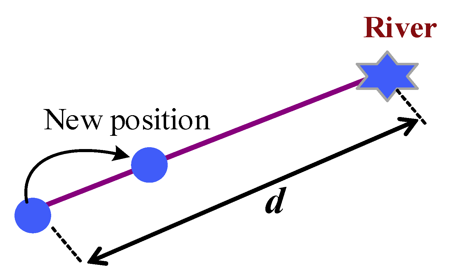
3.1. Water Cycle Algorithm
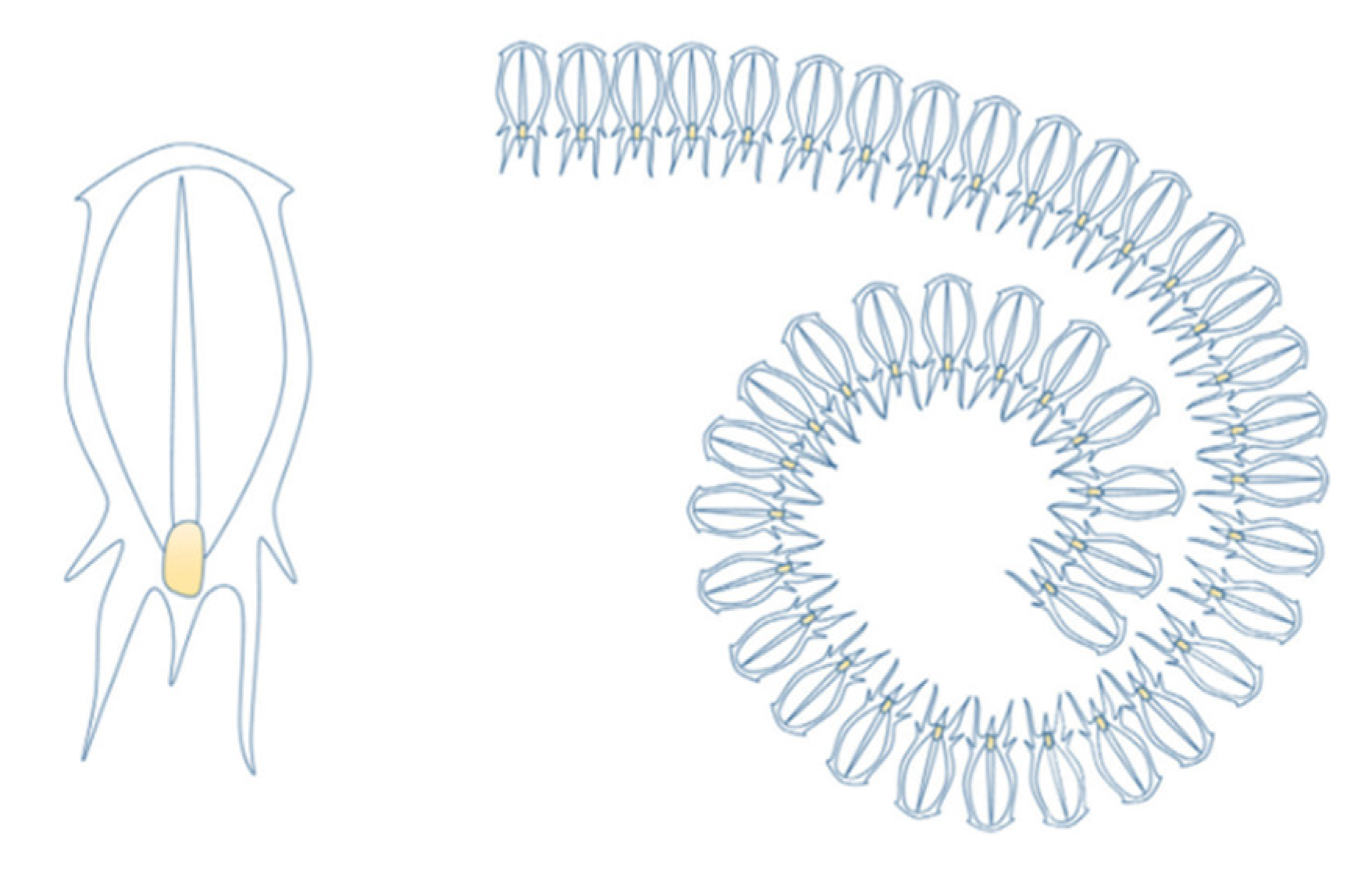
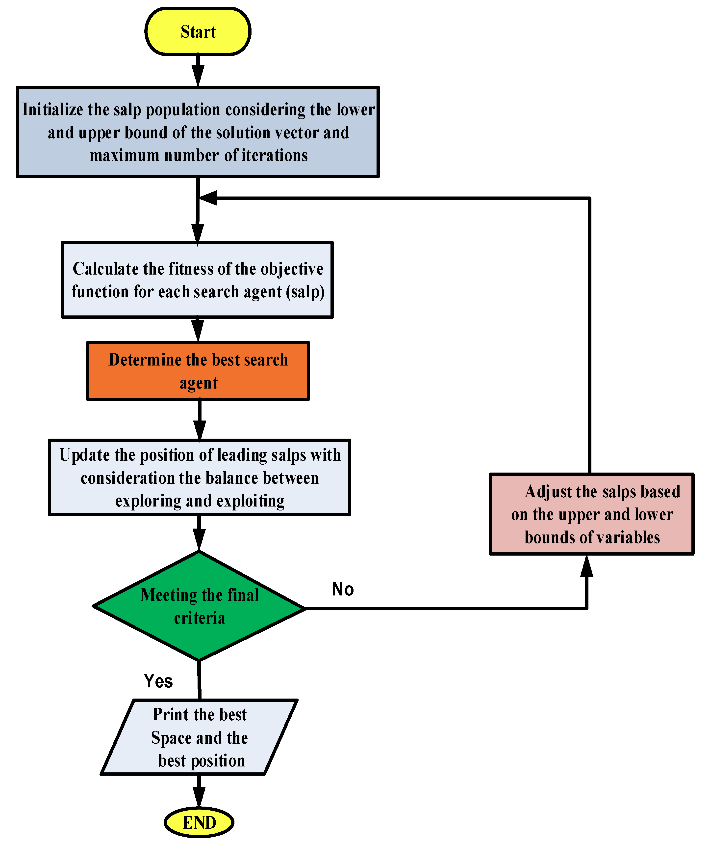
3.2. Salp Swarm Algorithm
3.3. Satin Bowerbird Optimization
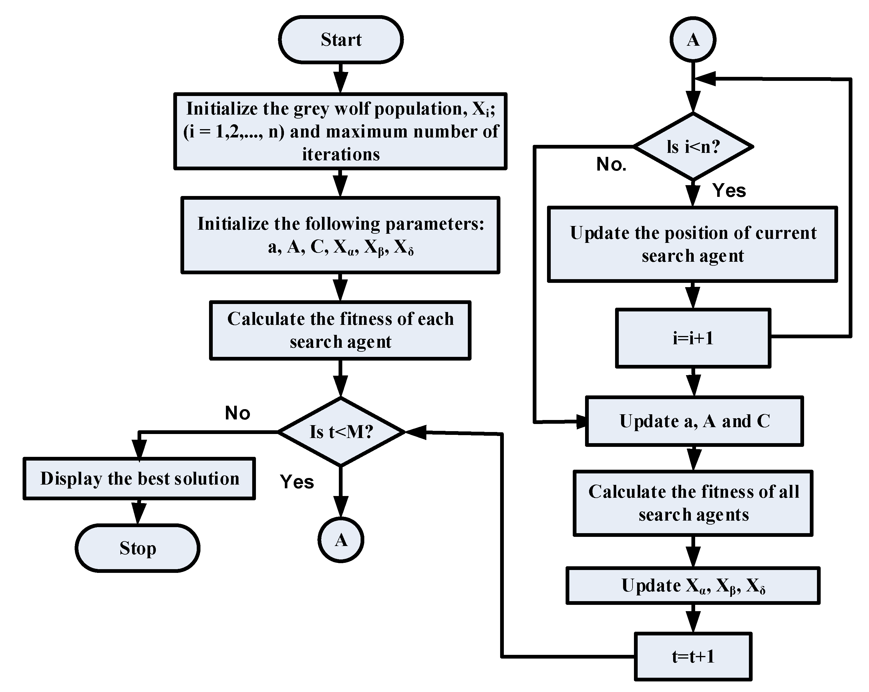
3.4. Grey Wolf Optimizer
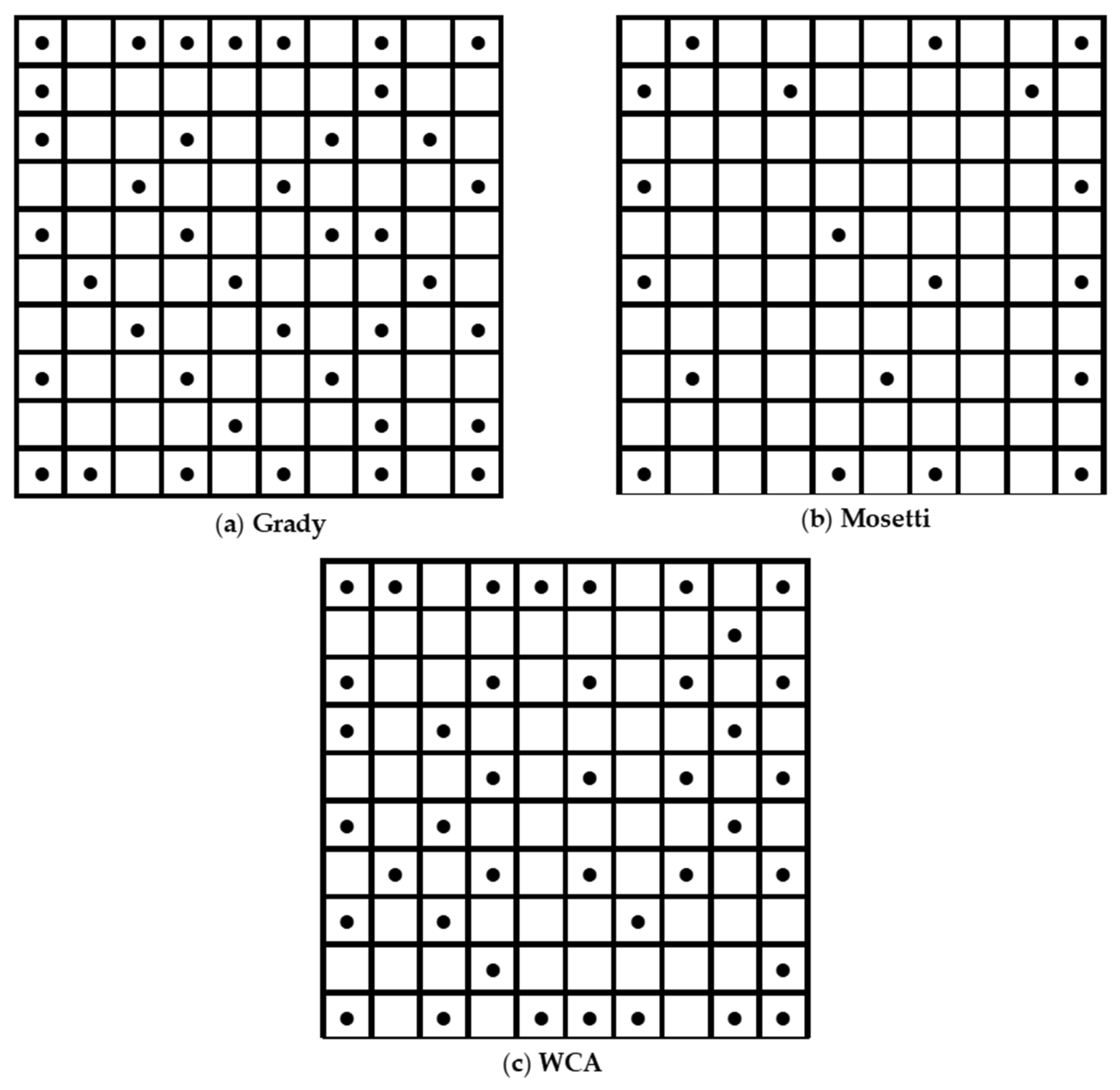
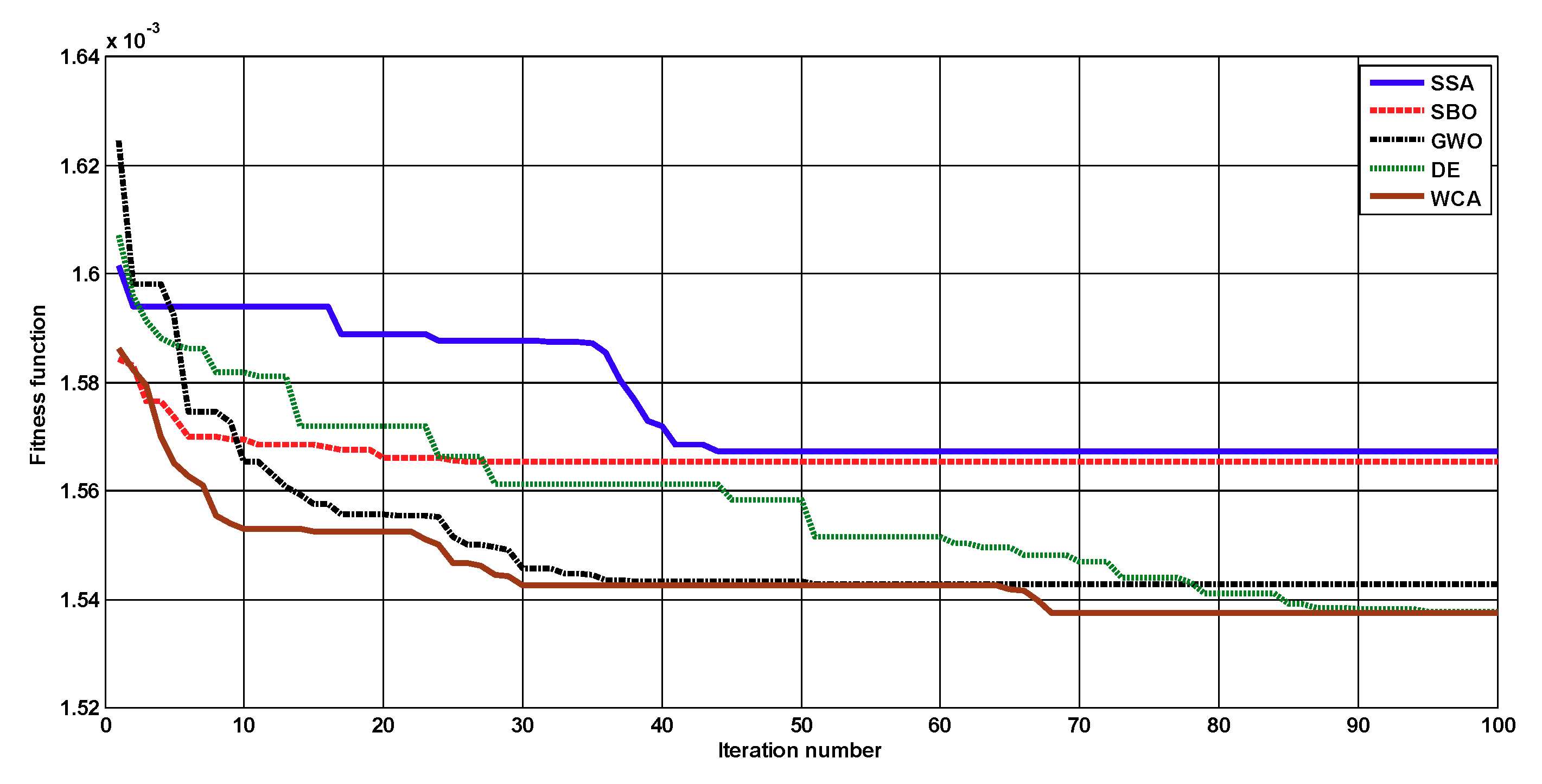
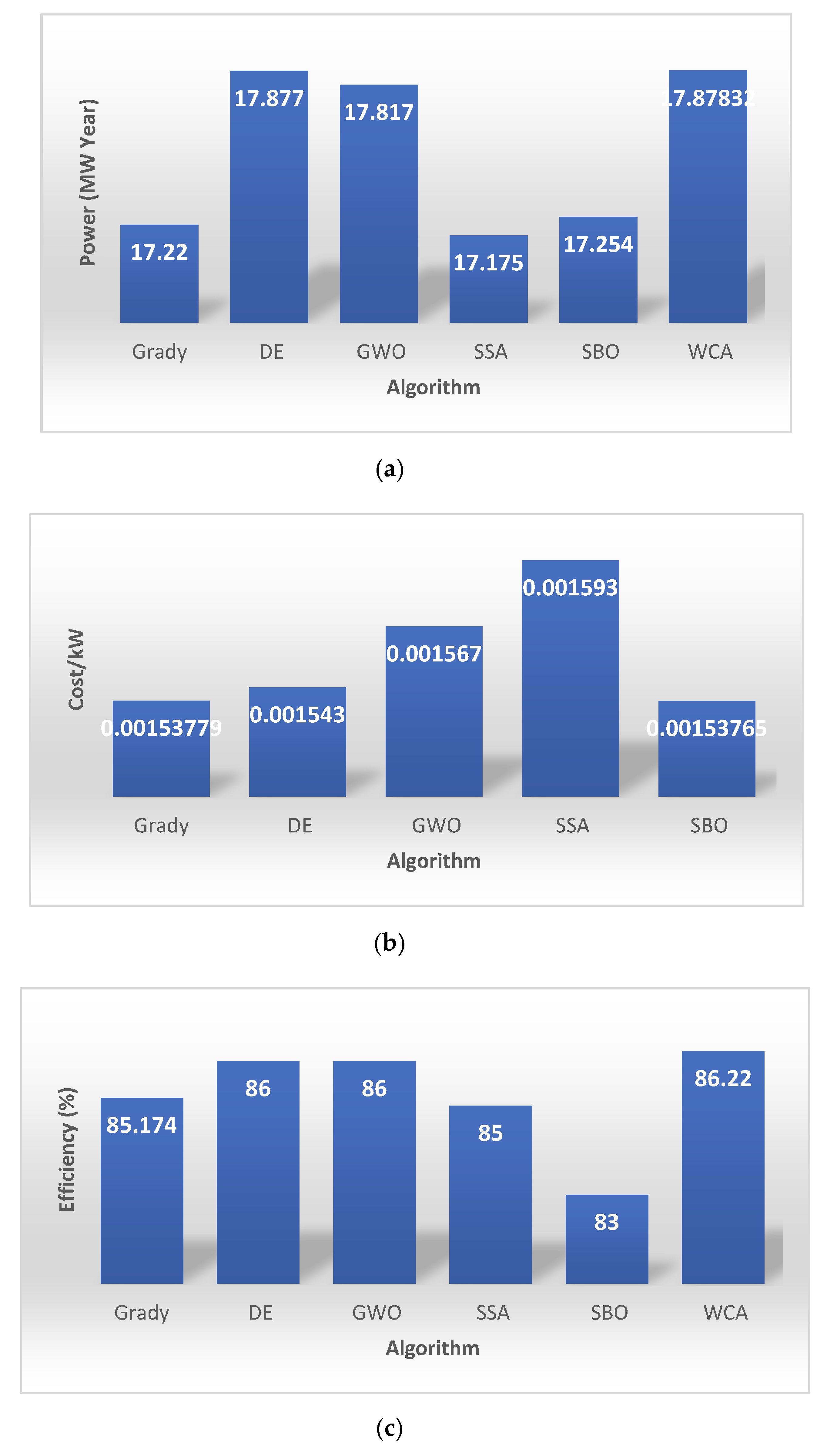
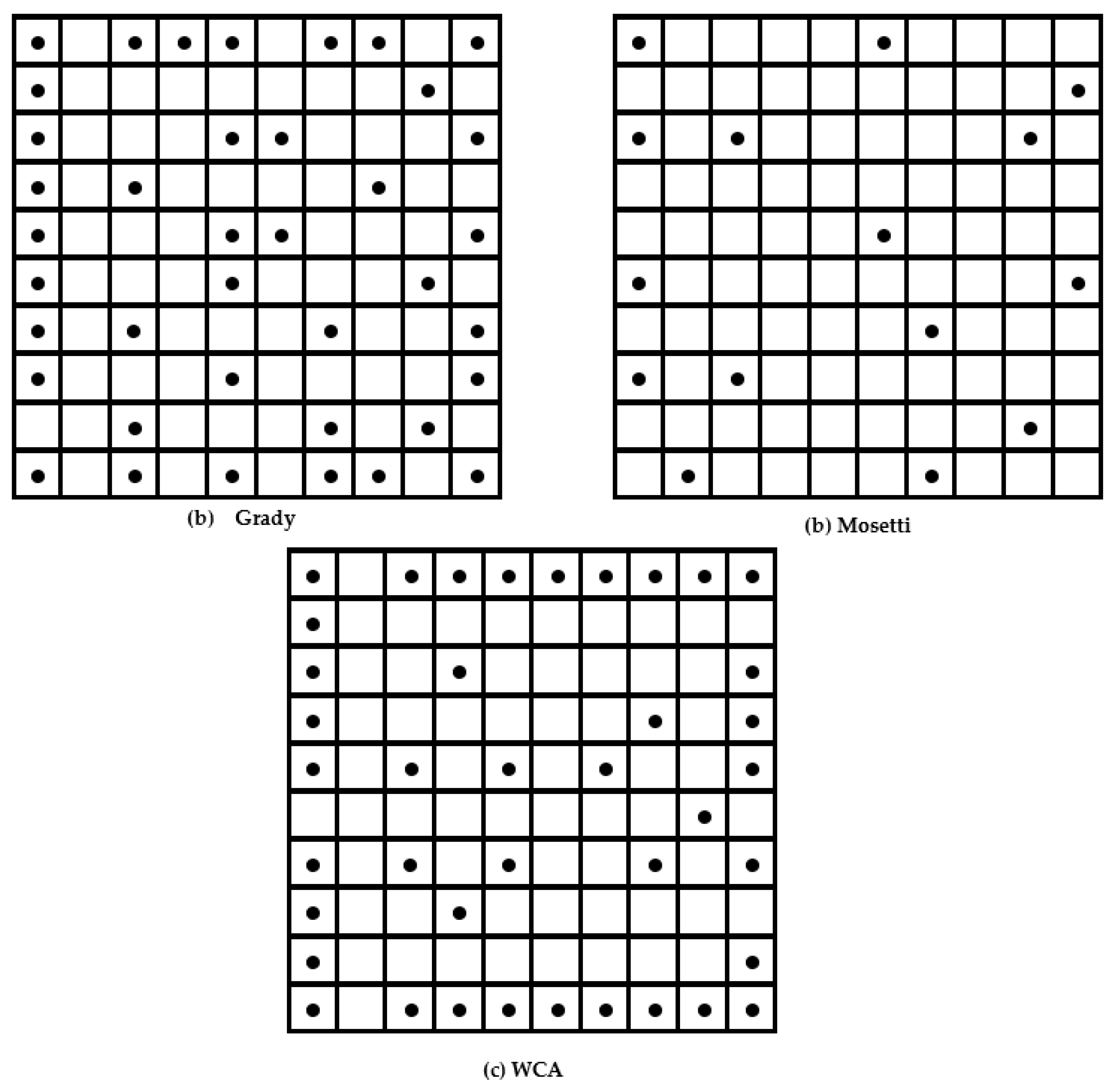
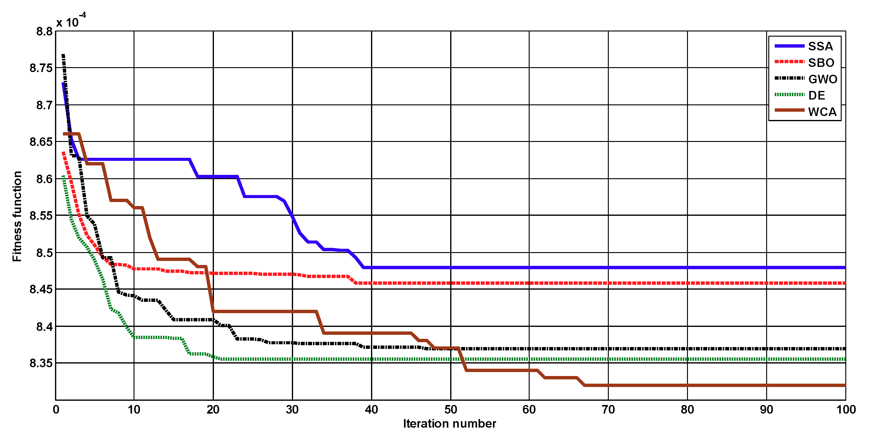
4. Results and Discussions
5. Conclusions
Author Contributions
Funding
Conflicts of Interest
References
- Marmoush, M.M.; Rezk, H.; Shehata, N.; Henry, J.; Gomaa, M.R. A novel merging Tubular Daylight Device with Solar Water Heater–Experimental study. Renew. Energy 2018, 125, 947–961. [Google Scholar] [CrossRef]
- Rezk, H.; El-Sayed, A.M. Sizing of a stand-alone concentrated photovoltaic system in Egyptian site. Electrical Power Energy Syst. 2013, 45, 325–330. [Google Scholar] [CrossRef]
- Rezk, H. A comprehensive sizing methodology for stand-alone battery-less photovoltaic water pumping system under the Egyptian climate. J. Cogent Eng. 2016, 3. [Google Scholar] [CrossRef]
- Rezk, H.; Dousoky, G.M. Technical and economic analysis of different configurations of stand-alone hybrid renewable power systems—A case study. Renew. Sustain. Energy Rev. 2016, 62, 941–953. [Google Scholar] [CrossRef]
- Hemeida, M.G.; Rezk, H.; Hamada, M.M. A comprehensive comparison of STATCOM versus SVC-based fuzzy controller for stability improvement of wind farm connected to multi-machine power system. Electr. Eng. 2018, 100, 935–951. [Google Scholar] [CrossRef]
- Renewables 2018 Global Status Report. Available online: http://www.ren21.net/status-of-renewables/global-status-report/ (accessed on 2 November 2018).
- Bastankhah, M.; Porté-Agel, F. A new analytical model for wind-turbine wakes. Renew. Energy 2014, 70, 116–123. [Google Scholar] [CrossRef]
- Khanali, M.; Ahmadzadegan, S.; Omid, M.; Nasab, F.K.; Chau, K.W. Optimizing layout of wind farm turbines using genetic algorithms in Tehran province, Iran. Int. J. Energy Environ. Eng. 2018, 9, 399–411. [Google Scholar] [CrossRef]
- Biswas, P.P.; Suganthan, P.N.; Amaratunga, G.A.J. Optimization of Wind Turbine Rotor Diameters and Hub Heights in a Windfarm Using Differential Evolution Algorithm. In Proceedings of Sixth International Conference on Soft Computing for Problem Solving; Advances in Intelligent Systems and Computing; Springer: Singapore, 2017; Volume 547. [Google Scholar]
- DuPont, B.; Cagan, J.; Moriarty, P. An advanced modeling system for optimization of wind farm layout and wind turbine sizing using a multi-level extended pattern search algorithm. Energy 2016, 106, 802–814. [Google Scholar] [CrossRef]
- Grady, S.A.; Hussaini, M.Y.; Abdullah, M.M. Placement of wind turbines using genetic algorithms. Renew. Energy 2005, 30, 259–270. [Google Scholar] [CrossRef]
- Emami, A.; Noghreh, P. New approach on optimization in placement of wind turbines within wind farm by genetic algorithms. Renew. Energy 2011, 35, 1559–1564. [Google Scholar] [CrossRef]
- Chen, Y.; Li, H.; Jin, K.; Song, Q. Wind farm layout optimization using genetic algorithm with different hub height wind turbines. Energy Convers. Manag. 2013, 70, 56–65. [Google Scholar] [CrossRef]
- Shakoor, R.; Hassan, M.Y.; Raheem, A.; Rasheed, N.; Mohd, N. Wind farm layout optimization by using Definite Point selection and genetic algorithm. In Proceedings of the 2014 IEEE International Conference on Power and Energy (PECon), Kuching, Malaysia, 1–3 December 2014; pp. 191–195. [Google Scholar]
- Turner, S.D.O.; Romero, D.A.; Zhang, P.Y.; Amon, C.H.; Chan, T.C.Y. A new mathematical programming approach to optimize wind farm layouts. Renew. Energy 2004, 63, 674–680. [Google Scholar] [CrossRef]
- Gao, X.; Yang, H.; Lin, L.; Koo, P. Wind turbine layout optimization using multi-population genetic algorithm and a case study in Hong Kong offshore. J. Wind Eng. Ind. Aerodyn. 2015, 139, 89–99. [Google Scholar] [CrossRef]
- Eroğlu, Y.; Seçkiner, S.U. Design of wind farm layout using ant colony algorithm. Renew. Energy 2012, 44, 53–62. [Google Scholar] [CrossRef]
- Chowdhury, S.; Zhang, J.; Messac, A.; Castillo, L. Unrestricted wind farm layout optimization (UWFLO): Investigating key factors influencing the maximum power generation. Renew. Energy 2012, 38, 16–30. [Google Scholar] [CrossRef]
- Feng, J.; Shen, W.Z. Solving the wind farm layout optimization problem using random search algorithm. Renew. Energy 2015, 78, 182–192. [Google Scholar] [CrossRef]
- Marmidis, G.; Lazarou, S.; Pyrgioti, E. Optimal placement of wind turbines in a wind park using Monte Carlo simulation. Renew. Energy 2008, 33, 1455–1460. [Google Scholar] [CrossRef]
- Mora, J.C.; Barón, J.M.C.; Santos, J.M.R.; Payán, M.B. An evolutive algorithm for wind farm optimal design. Neurocomputing 2007, 70, 2651–2658. [Google Scholar] [CrossRef]
- Wolpert, D.H.; Macready, W.G. No free lunch theorems for optimization. IEEE Trans. Evol. Comput. 1997, 1, 67–82. [Google Scholar] [CrossRef]
- Tolba, M.; Rezk, H.; Diab, A.; Al-Dhaifallah, M. A Novel Robust Methodology Based Salp Swarm Algorithm for Allocation and Capacity of Renewable Distributed Generators on Distribution Grids. Energies 2018, 11, 2556. [Google Scholar] [CrossRef]
- Eskandar, H.; Sadollah, A.; Bahreininejad, A.; Hamdi, M. Water cycle algorithm—A novel metaheuristic optimization method for solving constrained engineering optimization problems. Comput. Struct. 2012, 110, 151–166. [Google Scholar] [CrossRef]
- Mirjalili, S.; Gandomi, A.; Mirjalili, S.Z.; Saremi, S.; Faris, H.; Mirjalili, S.M. Salp Swarm Algorithm: A bio-inspired optimizer for engineering design problems. Adv. Eng. Softw. J. 2017, 114, 163–191. [Google Scholar] [CrossRef]
- Hamid, S.S.M.; Khatibi, V.B. Satin bowerbird optimizer: A new optimization algorithm to optimize ANFIS for software development effort estimation. Eng. Appl. Artif. Intell. 2017, 60, 1–15. [Google Scholar] [CrossRef]
- Mosetti, G.; Poloni, C.; Diviacco, B. Optimization of wind turbine positioning in large wind farms by means of a genetic algorithm. J. Wind Eng. Ind. Aerodyn. 1994, 51, 105–116. [Google Scholar] [CrossRef]
- Rezk, H.; Fathy, A. A novel optimal parameters identification of triple-junction solar cell based on a recently meta-heuristic water cycle algorithm. Sol. Energy 2017, 157, 778–791. [Google Scholar] [CrossRef]
- Mohamed, M.A.; Diab, A.A.Z.; Rezk, H. Partial shading mitigation of PV systems via different meta-heuristic techniques. Renew. Energy 2018, 130, 1159–1175. [Google Scholar] [CrossRef]
- Chintam, J.R.; Daniel, M. Real-Power Rescheduling of Generators for Congestion Management Using a Novel Satin Bowerbird Optimization Algorithm. Energies 2018, 11, 183. [Google Scholar] [CrossRef]
- Li, Q.; Chen, H.; Huang, H.; Zhao, X.; Cai, Z.; Tong, C.; Liu, W.; Tian, X. An enhanced grey wolf optimization based feature selection wrapped kernel extreme learning machine for medical diagnosis. Comput. Math. Methods Med. 2017. [Google Scholar] [CrossRef]
- Zaki Diab, A.A.Z.; Rezk, H. Optimal Sizing and Placement of Capacitors in Radial Distribution Systems Based on Grey Wolf, Dragonfly and Moth–Flame Optimization Algorithms. Iran. J. Sci. Technol. Trans. Electr. Eng. 2019, 43, 77–96. [Google Scholar] [CrossRef]


| Author | Year | Optimizer | Remarks |
|---|---|---|---|
| Khanali [8] | 2018 | Genetic algorithms | Actual wind speed data of Tehran were considered. The main finding was that the longitudinal space among WTs must be larger than the latitudinal distance in order to increase WF performance. The efficiency of WF was 89.5%. |
| Biswas [9] | 2017 | Differential evolution algorithm | The fitness function was the maximization of system efficiency. The decision variables were rotor diameters and hub heights. |
| Bryony [10] | 2016 | Pattern search algorithm | Two different cases of wind were considered: (1) constant value and direction and (2) three different values and directions. |
| Grady [11] | 2005 | Genetic algorithms | The two-dimensional Park model proposed by Jensen was used. The total cost of WF was minimized and at the same time the harvested energy was maximized. |
| Emami [12] | 2010 | Genetic algorithms | The capital cost of WF was considered as objective function. |
| Chen [13] | 2013 | Genetic algorithm | WTs with different hub heights were considered. The main conclusion was that employing WTs with different hub heights can increase power output in small WFs. Different cost models were considered. |
| Shakoor [14] | 2014 | Genetic algorithm | The linear Jensen’s wake model was employed with definite selection criteria. |
| Turner [15] | 2014 | New mathematical programming | Both linear and quadratic formulas for optimization were considered. |
| Gao [16] | 2015 | Multipopulation genetic algorithm | Real data from offshore Hong Kong was collected. The WF performance was improved. |
| Eroğlu [17] | 2012 | Ant colony optimization (ACO) | The study showed that employing ACO can help improve the performance of WFs. |
| Chowdhury [18] | 2012 | Particle swarm optimization | The presented approach was not applied on a large scale. The work presented an experimental prototype. |
| Feng [19] | 2015 | Random search algorithm | The proposed strategy was found to be useful for WFs that had a constant number of WTs. |
| Marmidis [20] | 2008 | Monte Carlo simulation | A small-scale wind farm was used as case study. The results did not depend on real data. |
| Mora et al. [21] | 2007 | Evolutionary algorithm | The capital investment of WF was considered. Different economic factors were also considered. |
| Parameter | Value |
|---|---|
| Hub height (z) | 60 m |
| Rotor radius (r0) | 20 m |
| Thrust coefficient | 0.88 |
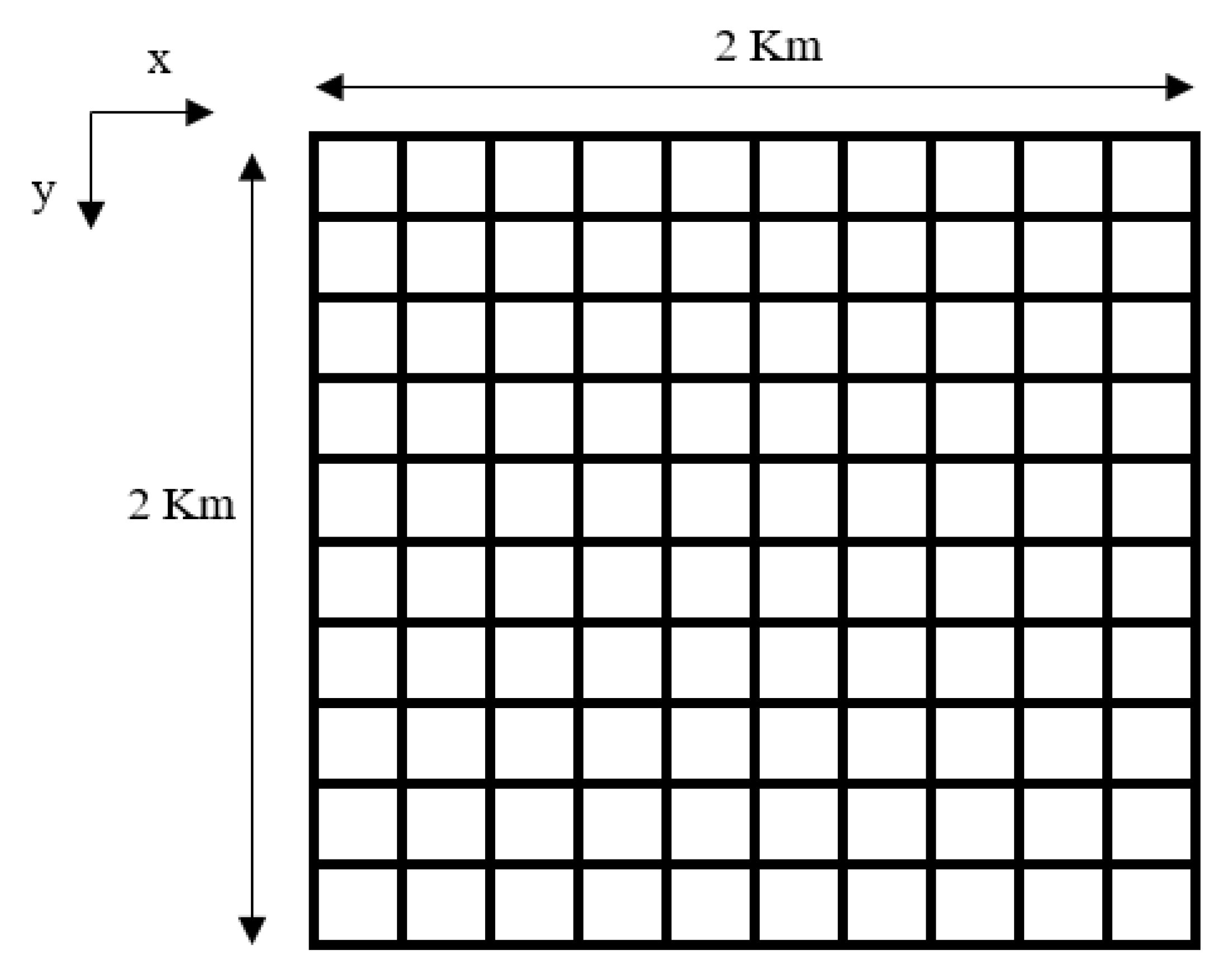
| WF area | 2 Km × 2 Km |
| Air density | 1.2254 kg/m3 |
| Rotor efficiency | 0.4 |
| Method | Number of Turbines | Pt (kW Year) | Cost/W ($) | Efficiency (%) |
|---|---|---|---|---|
| Grady [11] | 39 | 17,220 | 1.567 | 85.174 |
| Mosetti [27] | 19 | 9244 | 1.736 | NA |
| Feng (1) [19] | 39 | 17,406 | 1.547 | NA |
| DE | 40 | 17,877 | 1.538 | 86 |
| GWO | 40 | 17,817 | 1.543 | 86 |
| SSA | 39 | 17,175 | 1.567 | 85 |
| SBO | 40 | 17,254 | 1.593 | 83 |
| WCA | 40 | 17,878.32 | 1.538 | 86.22 |
| Method | Number of Turbines | Pt (kW Year) | Cost/W ($) | Efficiency (%) |
|---|---|---|---|---|
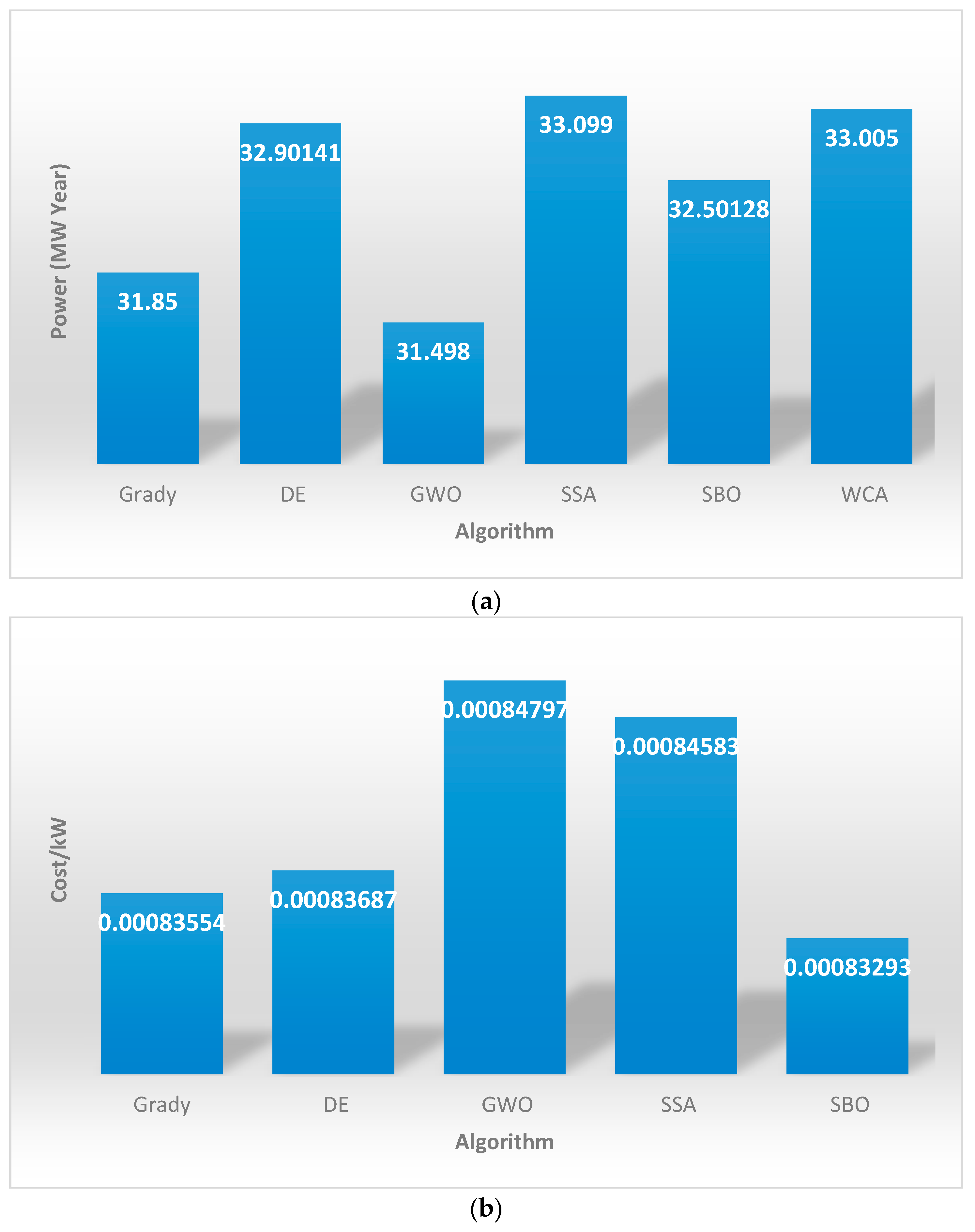
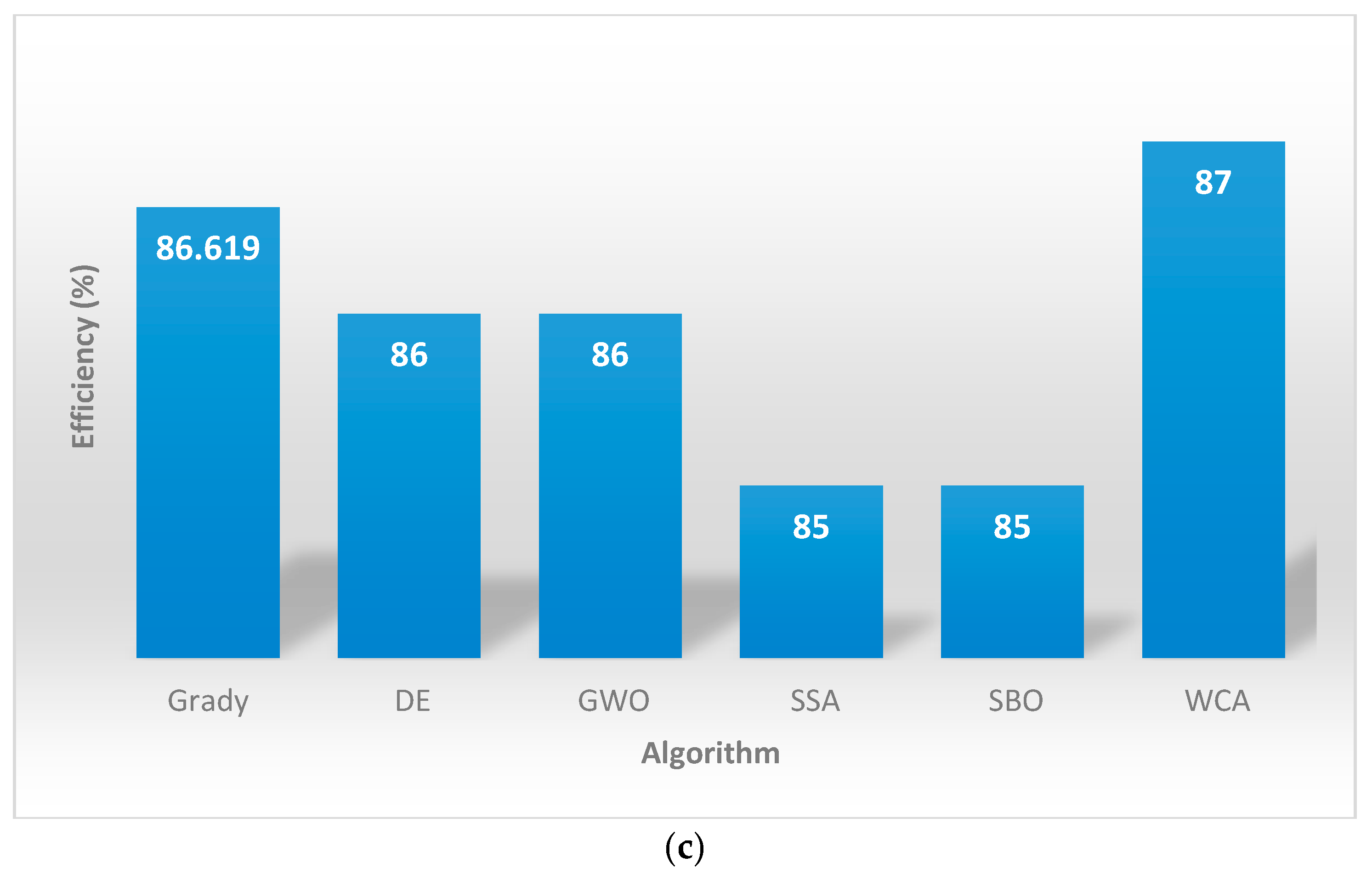
| Grady [11] | 39 | 31,850 | 0.840 | 86.619 |
| Mosetti [27] | 15 | 13,460 | 0.994 | NA |
| Feng (1) [19] | 39 | 32,096 | 0.839 | NA |
| DE | 40 | 32,901.41 | 0.836 | 86 |
| GWO | 38 | 31,498 | 0.837 | 86 |
| SSA | 41 | 33,099 | 0.848 | 85 |
| SBO | 40 | 32,501.28 | 0.846 | 85 |
| WCA | 40 | 33,005 | 0.833 | 87 |
© 2019 by the authors. Licensee MDPI, Basel, Switzerland. This article is an open access article distributed under the terms and conditions of the Creative Commons Attribution (CC BY) license (http://creativecommons.org/licenses/by/4.0/).
Share and Cite
Rezk, H.; Fathy, A.; Diab, A.A.Z.; Al-Dhaifallah, M. The Application of Water Cycle Optimization Algorithm for Optimal Placement of Wind Turbines in Wind Farms. Energies 2019, 12, 4335. https://doi.org/10.3390/en12224335
Rezk H, Fathy A, Diab AAZ, Al-Dhaifallah M. The Application of Water Cycle Optimization Algorithm for Optimal Placement of Wind Turbines in Wind Farms. Energies. 2019; 12(22):4335. https://doi.org/10.3390/en12224335
Chicago/Turabian StyleRezk, Hegazy, Ahmed Fathy, Ahmed A. Zaki Diab, and Mujahed Al-Dhaifallah. 2019. "The Application of Water Cycle Optimization Algorithm for Optimal Placement of Wind Turbines in Wind Farms" Energies 12, no. 22: 4335. https://doi.org/10.3390/en12224335
APA StyleRezk, H., Fathy, A., Diab, A. A. Z., & Al-Dhaifallah, M. (2019). The Application of Water Cycle Optimization Algorithm for Optimal Placement of Wind Turbines in Wind Farms. Energies, 12(22), 4335. https://doi.org/10.3390/en12224335