Article

Insight into the Pore Characteristics of a Saudi Arabian Tight Gas Sand Reservoir

Center for Integrative Petroleum Research, King Fahd University of Petroleum & Minerals, Dhahran 31261, Saudi Arabia
*
Authors to whom correspondence should be addressed.
Energies 2019, 12(22), 4302; https://doi.org/10.3390/en12224302
Submission received: 9 October 2019 / Revised: 27 October 2019 / Accepted: 29 October 2019 / Published: 12 November 2019
(This article belongs to the Special Issue Development of Unconventional Reservoirs)

Abstract

:
The petrophysical characterization of tight gas sands can be affected by clay minerals, gas adsorption, microfractures, and the presence of high-density minerals. In this study, we conducted various petrophysical, petrographic, and high-resolution image analyses on Saudi Arabian tight sand in order to understand how a complex pore system responds to measurement tools. About 140 plug samples extracted from six wells were subjected to routine core analyses including cleaning, drying, and porosity–permeability measurements. The porosity–permeability data was used to identify hydraulic flow units (HFU). In order to probe the factors contributing to the heterogeneity of this tight sand, 12 subsamples representing the different HFUs were selected for petrographic study and high-resolution image analysis using SEM, quantitative evaluation of minerals by scanning electron microscope (QEMSCAN), and micro-computed tomography (µCT). Nuclear magnetic resonance (NMR) and electrical resistivity measurements were also conducted on 56 subsamples representing various lithofacies. NMR porosity showed good agreement with other porosity measurements. The agreement was remarkable in specific lithofacies with porosity ranging from 0.1% to 7%. Above this range, significant scatters were seen between the porosity methods. QEMSCAN results revealed that samples with <7% porosity contain a higher proportion of clay than those with porosity >7%, which are either microfractured or contain partially dissolved labile minerals. The NMR T2 profiles also showed that samples with porosity <7% are dominated by micropores while samples with porosity >7% are dominated by macropores. Analysis of the µCT images revealed that pore throat sizes may be responsible for the poor correlation between NMR porosity and other porosity methods. NMR permeability values estimated using the Shlumberger Doll Research (SDR) method are fairly correlated with helium permeability (with an R2 of 0.6). Electrical resistivity measurements showed that the different rock types fall on the same slope of the formation factors versus porosity, with a cementation factor of 1.5.

Graphical Abstract

1. Introduction

Population growth and the associated need for sustainable sources of energy have led to an increased interest in the exploration and production from unconventional resources in the recent years. Only four countries—Canada, the USA, China, and Argentina—have fully developed unconventional gas from either shale or tight gas reservoirs [1]. The kingdom of Saudi Arabia is believed to have the fifth largest reserves of unconventional gas [1]. It is also estimated that the kingdom’s unconventional gas resources could be as high as 10 times the conventional gas resources [2]. Hence, unconventional gas development is expected to grow exponentially in the kingdom [1]. In Saudi Arabia, tight gas is believed to have more favorable geology than shale because the tight gas deposits are largely found in sandstones with higher permeability and porosity than shale. The bulk mineralogical composition of sandstone, which is dominantly comprised of quartz with or without subordinate amount of feldspars and relatively low clay content, make the tight sand gas reservoirs easier and cheaper to hydraulically fracture than clay-rich oil shale or shale gas reservoirs. However, these tight sands are highly heterogeneous such that an extensive amount of field and laboratory data are required to understand the properties of different reservoir types and to design the appropriate stimulation methods. Improved petrophysical knowledge and methods of low permeability rocks are essential elements toward a successful development of unconventional reservoirs. The most important rock properties that must be known are pay zone thickness, porosity, permeability, water saturation, in-situ stresses, and young modulus [3]. These properties are determined from well logs, well tests, laboratory core measurements, drilling records, etc. Laboratory measurements are the most direct and reliable source of data.
The accurate measurement of porosity and permeability is crucial in all types of reservoir rocks. These measurements are essential for assessing the volume of hydrocarbon in place and the productivity of wells drilled through them. The measurements are also used to calibrate downhole-logging tools. Measurement accuracy is more crucial in very low-porosity and low-permeability rocks such as tight sand or shales [4]. The small unconnected pores present in complex mineralogy and organic matters of unconventional reservoirs (tight sand and shale gas) make their porosity and permeability measurement problematic [5,6]. The presence of accessory minerals, clay types, clay swelling, fine migration, gas slippage effect (or Klinkenberg effect), and turbulence (or Forchiemer’s effect) further complicates the accuracy of measuring these reservoir properties. The presence of clay (especially montmorillonite) can be a worrisome obstacle in achieving the desired measurement accuracy [7]. Clays have large surface areas that contain adsorbed water that do not contribute to the accessible storage space of the rock. The accessible storage space is the effective porosity of the rock. Hence, for petrophysical study such as electrical resistivity, permeability, and capillary pressure, it is essential to preserve the clay structure during sample preparation and saturation.
Laboratory analysis in most cases requires that the extracted rock samples be cleaned with solvents, oven dried, and resaturated with synthetic formation fluids as part of a workflow to restore them to their native conditions. Drying can cause the irreversible destruction of the clay fabric and eventually an increase in the porosity and permeability of the samples. To accurately determine porosity types (micropores and mesopores) and their impacts on mud rocks, it is important to follow sample preparation and experimental protocols that would preserve the physical structures of the samples [8]. Contact with incompatible fluids other than their native fluids can cause a variety of problems such as clay swelling, fine migration, and the plugging of pore throats, and ultimately a reduction in the porosity and permeability values. Therefore, it is important to preserve the clay structure during drying such that the clay can be rehydrated to its original state. Morrow et al. [9] showed that clay microstructure (microporosity) can still be partially preserved at temperatures up to 500 °C. However, beyond this temperature the clay structure begins to collapse with a total collapse occurring at over 1000 °C. For a preserved clay structure, the available cations on the clay surface will hydrate when resaturated. The degree of hydration depends on the original cations present at the cation exchange site of the clay. Sodium ion (Na+) is the most readily exchangeable cation, and in smectite it can cause adsorption of up to 32 layers of water molecules. In samples with large smectitie content, this large expansion after water adsorption can block pore throats and ultimately reduce sample permeability and porosity. Paramagnetic, ferromagnetic, and conductive minerals such as pyrites, hematite, and siderite in tight sandstones are also influencing factors in the rock response to important logging tools such as nuclear magnetic resonance, electrical resistivity, etc. Therefore, it is important that laboratory measurements follow important protocols during the measurements of these sensitive formations. Nonetheless, analyses of tight rocks can further be complicated by their complex pore topology/heterogeneity.
The Saudi Arabia late Ordovician Sarah Formation is a glacial deposit in the northern part of the Rub’ al Khali basin. It is a proven gas reservoir in the northwestern and central parts of Saudi Arabia that is being explored as a potential tight gas sandstone reservoir. The formation’s paleovalleys cut deeply into the basement and older Paleozoic succession, including Saq formation and all the members of the Qasim Formation including Hanadir, Khafah, Ra’an, and Quwarah members (Figure 1) in northwest and central Saudi Arabia [10,11]. The sub-Sarah unconformity above the underlying Saq and Qasim Formations [10] marks the basal boundary of this formation while the basal occurrence of the Qusaiba Hot Shale delineates its upper contact. The formation is dominantly comprised of pebbly, poorly sorted, fine to coarse-grained, parallel, trough, and planar cross-bedded sandstones. Al-Harbi and Khan [11] described the sandstone as predominantly quartz arenite.
Sedimentological and petrographical analyses previously conducted on core samples from this formation revealed the occurrences of various lithofacies, which were grouped into four facies associations (FAs) (as shown in Figure 2). The facies association are massive to ripple-laminated sandstone (FA1), gray massive sandstone (FA2), diamictites (FA3), and partially deformed, massive-graded sandstone (FA4), which are interpreted as fluvial, glaciofluvial, glaciolacustrine delta, and subglacial outwash deposits, respectively [12]. Alqubalee et al. [13] reported that the clay and cement content in the fluvial facies (well A) and glaciofluvial facies (well E) are relatively low; however, grain compaction, feldspar dissolution, and authigenic illite were observed in these FAs. The pores and pore throats in most of the glaciolacustrine delta (wells B and C) and subglacial facies (wells B, D, and F) were filled by anhydrite, siderite, barite, or detrital illite.
In this paper, we present the results of various petrographic, petrophysical, and high-resolution imaging investigations on the Sarah tight gas reservoir in the Rub’ al Khali basin. The measurements were conducted on 140 core plugs extracted from six wells (named well A to well F). First, the porosity and permeability of the samples were measured using pulse decay methods. Then, the flow zone indicator method was used to group the samples into distinct hydraulic flow units. Subsequently, thin-section petrography, scanning electron microscope (SEM), quantitative evaluation of minerals by scanning electron microscope (QEMSCAN), nuclear magnetic resonance (NMR), high-resolution micro-computed tomography (µCT) imaging, and electrical resistivity were conducted on subsamples representing the different flow units in order to understand the different reservoir rock types and the factors controlling their pore behavior. Since petrographic analysis on the samples showed that smectite clay exists in a very insignificant amount, the samples were cleaned and dried using conventional techniques. Nonetheless, the main clay fabrics are believed to be preserved based on the findings of Morrow et al. [9].

2. Methodology

2.1. Rock Sample Preparation

Cylindrical cores of 4-inch diameters were extracted from six wells: namely, well A, well B, well C, well D, well E, and well F. The six wells were drilled through the Sarah reservoir formation in the Rub’ al Khali basin. Samples from well A and well B were extracted at a depth of 16xxx feet, while samples from wells C and D were extracted at a depth of 17xxx feet. Samples from well E were extracted at a depth of 14xxx feet and those from well F were extracted at a depth of 18xxx feet. The wells drilled through a very heterogeneous reservoir with significant variation in porosity, permeability, and mineralogy. Then, cylindrical plugs of 1-inch and 1.5-inch diameter with lengths ranging from 1.5–4 inches were extracted from the cores. The plug samples were cleaned to remove hydrocarbon using a Soxhlet-type extractor circulating hot toluene and subsequently with alcohol to remove salt contaminants. The cleaned samples were dried in a vacuum oven. The Soxhlet extractor process involves evaporated toluene circulating through the pores of the rock specimen and thereby cleansing them of any oil present. This cleaning process was continued for several days to ensure a complete removal of residual hydrocarbon. To remove any traces of toluene and salt associated with the formation brine that might be remaining in the sample, the same Soxhlet extractor-cleaning procedure was repeated with isopropanol leach for at least 48 h. After cleaning with isopropanol, the rock specimens were dried under partial vacuum in a vacuum oven at 80 °C for about two days. Some vuggy core plugs or core plugs having surface irregularities, which cannot be used for porosity and permeability measurements under confining pressure, were repaired to remove the surface irregularities using rock powder mixed with epoxy. The average length and diameter of the core plugs were determined from five measurements at different points along the length and diameter, respectively. The averages of the length and diameter were used to calculate the bulk volume of each core plug. Then, the dry weights of the core plugs were measured using a weight balance accurate to 0.001 g.

2.2. Porosity and Permeability

Gas porosity was measured on the cleaned samples using an automated helium permeameter-porosimeter AP-608, which was calibrated using standard samples with known volume and a density of Berea sandstone and two billets of titanium and steel alloy. A high-purity (99.9%) helium gas was used to measure both porosity and permeability at a net confining pressure of 500 psi. Gas permeability, κg, was measured by injecting helium at a pore pressure of 200 psi, and the pressure was allowed to decay at a room temperature of 28 °C. Then, liquid permeability κl was calculated from the Klinkenberg [14] correlation shown in Equation (1) by plotting gas permeability measurements at different pressures against the reciprocal of the mean pressure 1/(pm−1). The intercept of the best-fit straight line with the gas permeability axis (at p ≈ ∞) is equal to liquid permeability:
κ =   κ g 1 + b p m
where k is the liquid permeability, kg is the gas permeability, pm is the mean pressure of flow, and b is the constant parameter (Klinkenberg’s slip factor for a given porous media).
Then, the core samples were saturated with brine solution at room temperature under a pressure of 2000 psi using a high-pressure vessel. Vacuum was used prior to saturation to remove trapped air from the samples. Each sample was left in the saturation vessel for about 48 h after which they were removed and gently wiped on a piece of paper in order to remove excess and surface water from the samples. Then, each sample was quickly weighted on a mass balance accurate to ±1 mg to determine the saturated mass (msat). Then, the pore volume occupied by brine, Vpore, was calculated as V pore = ( M sat M dry ) / ρ brine , while the gravimetric porosity was calculated as Φ g = V pore / V bulk . After weighting, the samples were quickly wrapped in thin plastic cling film to avoid drying and to allow NMR porosity experiments to be conducted on them. The composition of the synthetic brine used in saturating the samples fell within the range of the reservoir water samples extracted from the six wells (Table 1).

2.3. Petrographic and QEMSCAN Analyses

A total number of 140 thin sections selected from the studied core samples were prepared for petrographic study, where grain size, texture, and mineralogical composition (modal composition) were acquired. The concept of QEMSCAN, its applications, and its protocols have been explained and illustrated by several authors [15,16,17]. This advanced petrographic technique integrates scanning electron microscope (SEM), energy-dispersive spectroscopy, and species identification protocol (SIP)—a predefined spectral mineralogical library—to produce quantitative mineralogical maps from rock samples. We utilized the QEMSCAN technique to evaluate the mineralogical composition of some selected thin sections that represent the different petrophysical rock types in the reservoir. The thin sections were carbon coated using a Quorum EMS 150R ES before the analyses. A standard QEMSCAN setup was conducted, and the system was operated using an X-ray beam voltage of 15 kV and beam current of 10 nA (±0.05). The Field Image Scan mode on an area of 1 cm2 and 5-μm point spacing was selected. The QEMSCAN measurements took around 7.5 h. After that, the data was processed via iDiscover software, where field stitching, granulator, and boundary phase processors were applied.

2.4. Nuclear Magnetic Resonance Measurements

NMR measurements were performed on the samples using a low magnetic field NMR (0.05 Tesla and 2 MHz) ‘Geospec rock core analyzer’ from Oxford Instruments. The instrument was used to measure the T2 relaxation of the samples using optimized scanning parameters as follows: inter-echo spacing (Tau) value of 0.1 milliseconds, signal-to-noise ratio of 200, and a recycle delay of 11,250 milli seconds. T2 relaxation is a measure of the time that it takes for the transverse magnetization of a hydrogen nuclei to fall to approximately 37% of its initial value, after it was excited by a magnetic field in a direction transverse (perpendicular) to the magnetic field [18]. T2 is measured in milliseconds (ms), and it is related to the surface-to-volume ratio of the pores and the surface relaxivity ( ρ ) of the rock minerals coating the pore surface.
Since clay-rich rocks are sensitive to the type of water in contact with them, the synthetic brine used in saturating the rock samples prior to NMR measurements were prepared to simulate the actual reservoir fluid content. Water samples collected from several wells that were drilled through the study reservoir were analyzed for anion and cation compositions using inductive coupled plasma mass spectroscopy (ICP-MS) and inductive coupled plasma optical emission spectroscopy ICP-OES techniques, respectively. Table 1 shows the range of reservoir water properties and components. All TPH (total petroleum hydrocarbon) analysis was conducted on a wet weight basis. An Agilent GC 6890-N equipped with a flame ionization detector (FID) was used for the analysis.

2.5. High-Resolution Images of Samples

A laboratory µCT scanner, Versa XRM-5002D, was used to obtain tomographic images from small rock cuttings (rock cuttings of size approximately 8 mm × 10 mm) selected to represent the varieties of rock types present in the reservoir. X-rays from a microfocused source producing a polychromatic conical X-ray beam were used to generate images of the sample while employing a circular trajectory with 1601 projections. The scan voltage was set to 140 kV and power at 10 W with an exposure time of 1–4 s to achieve the optimal X-ray intensity flux count. The voxel resolution was kept constant around 3 µm for all the samples by adjusting the source and detector distance. Then, the µCT scans for all the samples were processed using PerGeos software.

2.6. Electrical Resistivity Measurements

Electrical resistivity measurements were conducted on the samples after NMR measurements using an electrical resistivity test system that allows the simultaneous measurement of 4-pole and 2-pole resistivity under elevated pressure and temperature. The system utilizes an Agilent 20-MHz waveform generator model 33,220 A to generate electrical currents over a wide range of frequencies, and a North Atlantic LCR meter model 2250 to measure samples’ inductance, capacitance, and resistance. Electrical resistivity measurements were conducted on the samples at 100% water saturation at a net confining pressure of 500 psi and at an ambient temperature of 25 °C.

3. Results and Discussions

3.1. Porosity and Permeability

Figure 3 and Figure 4 respectively show the histograms of the porosity and permeability of the studied samples. Figure 3 shows two distinct sample populations based on porosity data alone. The first group of samples has porosities ranging from 0.1%–7% with a modal value of 3%–4%. The samples in the second porosity group have porosities ranging between 7% and 13% with a modal value of 9%–10%. Statistical analysis of the samples’ permeabilities alone does not clearly show distinct groups of sample populations as was observed in the porosity data. Nonetheless, two groups of sample populations can be faintly seen based on the permeability values alone (independent of the porosity classification). As shown in Figure 4, one group of samples is very tight with permeability ranging between 0.001 and 0.2 mD (with a modal value of 0.03 mD). The second group of samples has permeability ranging between 0.2 and 1 mD (with a mode of 0.35 mD).

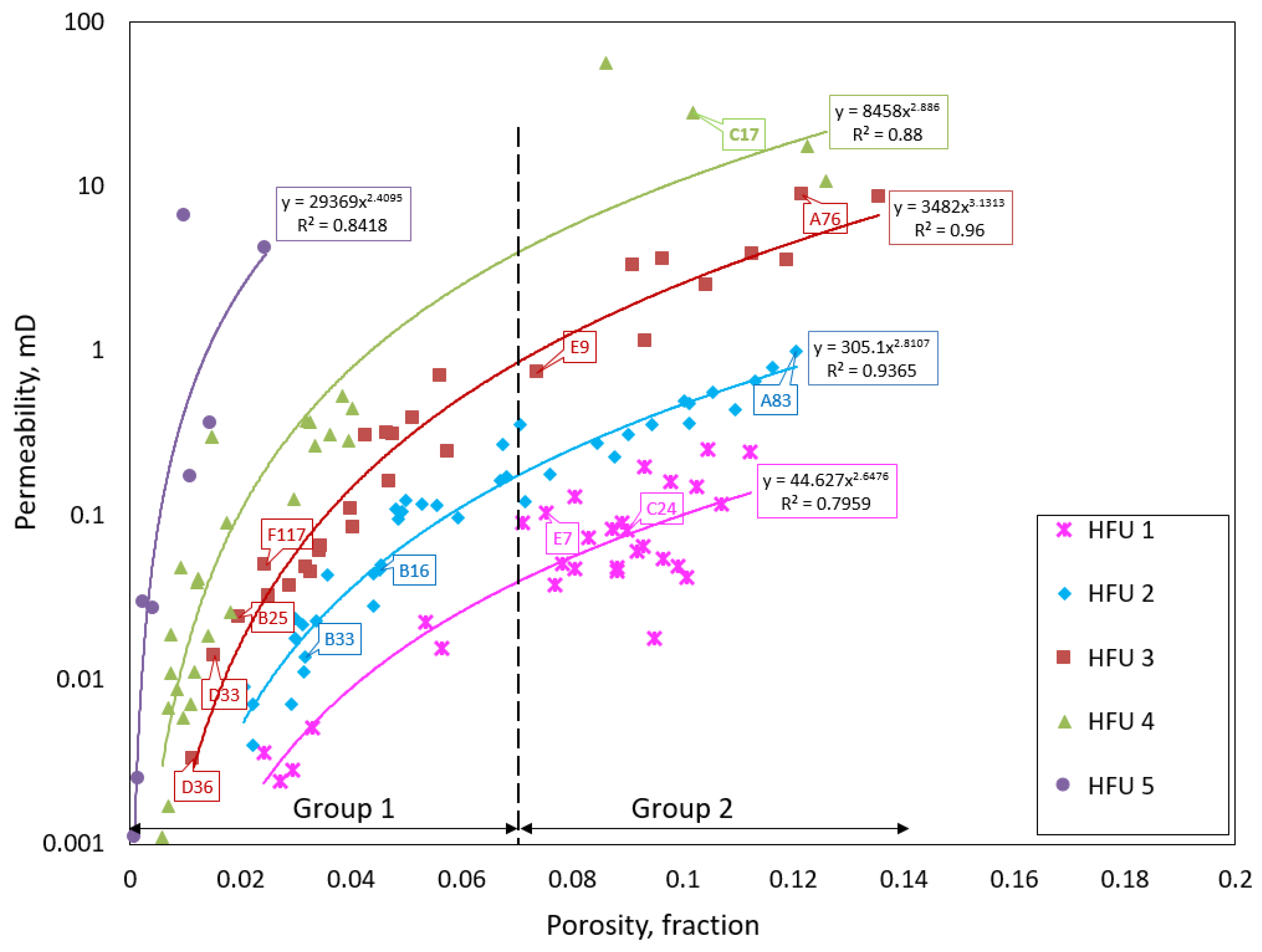
3.2. Porosity–Permeability Relationship

Figure 5 shows the cross-plot of porosity versus log of permeability for all 140 plugs extracted from the six wells (wells A–F). Most of the samples in porosity-group 1 (0.1%–7%) belong to rock samples extracted from wells D, E, and F (at a depth of 14,000–18,000 feet). All the plug samples extracted from well A (16,000 feet) belong to the porosity group 2 (7%–13%). Some of the plug samples from wells B and C belong to porosity group 1, while others belong to porosity group 2. There is no clear correlation between porosity and permeability (Figure 4). The scatter in the porosity–permeability cross-plot can be attributed to the variation in the type of facies, diagenesis, and petrophysical properties of the rocks. In Figure 5, the samples are color-coded based on the wells (and of course the depth) from which they were extracted. It can be seen that the low porosity is not associated with the depth from which the samples were extracted. In the next few subsections, the samples are also classified based on facies and petrophysical rock typing.

3.3. Facies Classification

As mentioned earlier, sedimentological and petrographical analyses conducted on core samples from the study formation revealed the occurrences of various lithofacies broadly classified into four facies associations (FAs), namely: (1) FA1, massive to ripple-laminated sandstone interpreted as fluvial; (2) FA2, gray massive sandstone (glaciofluvial); (3) FA3, diamictites (glaciolacustrine delta); and (4) FA4, partially deformed massive-graded sandstone (subglacial outwash deposits) [12,13]. The facies associations (FAs) are grossly heterogeneous (Figure 6A) and are also characterized by varied porosity distributions. Samples from FA1 and some samples from FA2 are characterized by primary interparticle porosity (Figure 6B), intraparticle porosity due to grain dissolution (Figure 6C), and microfracture porosity (Figure 6D). Their measured porosity values are greater than 7%. Petrographic examination of the FA1 samples indicates that they are dominantly subarkose arenite with authigenic pore-filling illite (Figure 6E). The low porosity values (<7%) encountered in the samples of the subglacial (FA3) and glaciofluvial (FA4) were probably due to the high matrix content (mainly detrital illite) and poor sorting. The presence of pore-filling anhydrite, barite (Figure 6F), siderite, and differential compaction in some of the FA2 and FA4 samples negatively impacted their reservoir quality.
Figure 7 shows the porosity–permeability plot of all the samples classified based on facies association. It is obvious that facies association FA4 exists exclusively in porosity group 1, while facies association FA1 exists only in porosity group 2. Facie associations FA2 and FA3 occur in both porosity groups. However, a clear correlation is not seen between porosity and permeability in any of the facies associations.

3.4. Petrophysical Rock Typing

In order to identify cores with identical pore and petrophysical characteristics, we used the concept of flow zone indicator (FZI) developed by Amaefule et al. [19]. They developed the FZI by rearranging the Kozeny–Carman equation, as shown in Equation (2):
K = ( e 3 ( 1 e ) 2 ) ( 1 K τ S V g r 2 )
where K is permeability (µm2), e is effective porosity, τ is tortuosity of flow path, and S V g r is the surface area per unit volume of grain.
Rearranging the equation by dividing both sides by porosity and taking the square root yields:
K =   1 S V g r 2 K τ ( e 1 e )
Amaefule et al. [19] expressed this equation as a reservoir quality index (RQI). If permeability is expressed in millidarcy (mD) and porosity is expressed as a fraction, the left-hand side of the equation becomes:
R Q I = 0.0314 K
Using Equation (4), the tortuosity and surface area of the rock samples in Equation (3) do not need to be measured, but rather replaced by the left-hand side of the same equation. The FZI is defined from Equation (3) as:
F Z I =   1 S V g r 2 K τ ( e 1 e )
Hence, R Q I = F Z I × z , where z =   e 1 e
On a log-log plot of RQI versus z (Figure 8), rock samples with the same hydraulic characteristics and similar petrophysical properties will align around a unit slope. The intercept of that slope in the RQI axis at the z value of 1 defines the flow zone for those samples. Samples with different FZI values will lie on other parallel lines. Hence, rocks having the same FZI tend to obey the same fluid distribution and fluid transport properties. Thus, they can be represented by the same petrophysical measurements such as relative permeability, capillary pressure, and electrical resistivity curves. The rock typing in Figure 8 showed five different hydraulic units. Classification of the rocks based on hydraulic flow units or a flow zones indicator revealed a clear power law correlation between porosity and the log of permeability in each hydraulic flow unit (Figure 9). The coefficients of regression (R2) range between 0.8 and 0.96. It also apparent from the cross-plot that the 7% cut-off value of porosity marks the deviation of the cross-plots from a linear trend. Further analysis using NMR, QEMSACN, and high-resolution imaging studies were used to probe this phenomenon, as presented in the subsequent subsections.

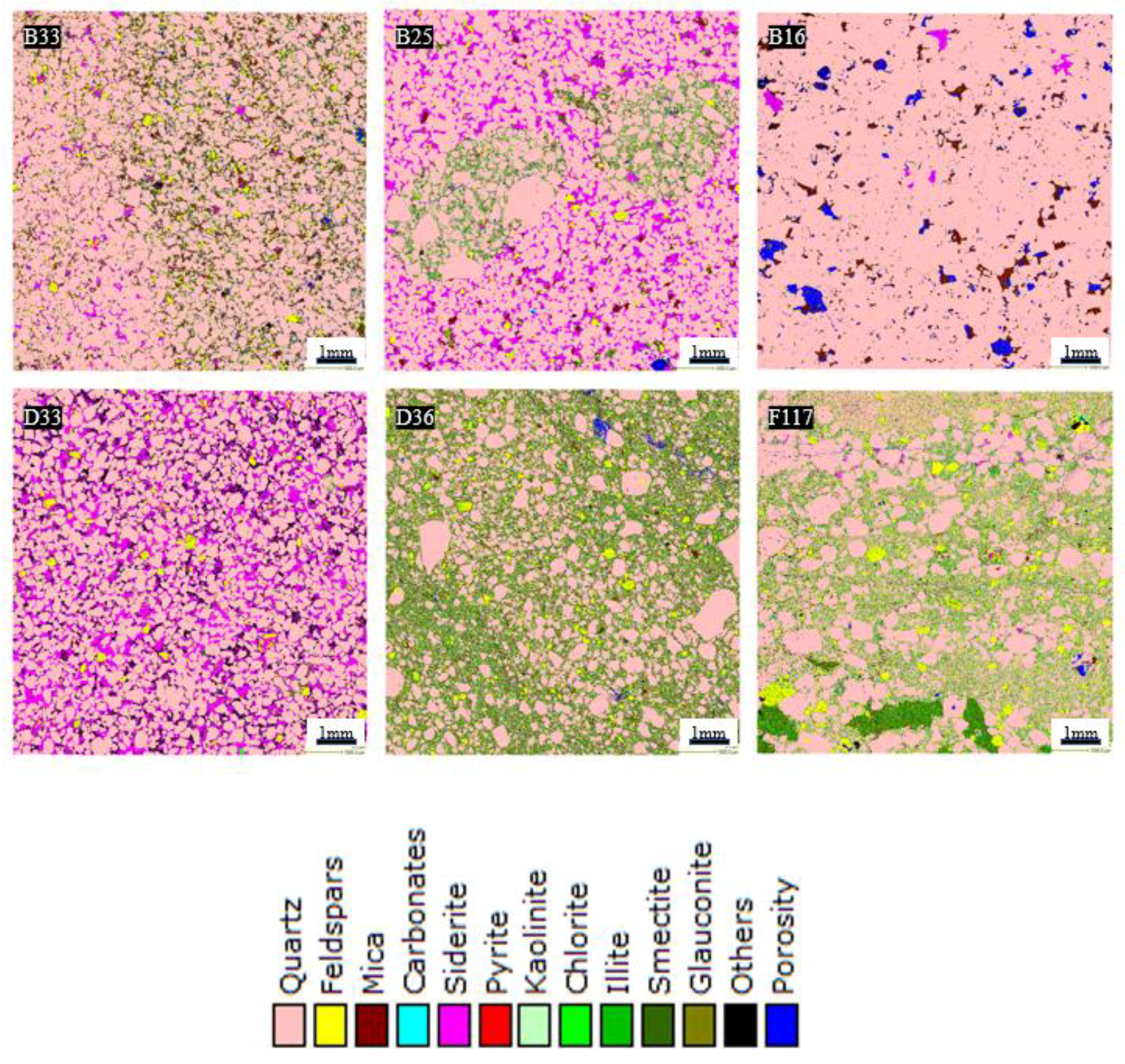
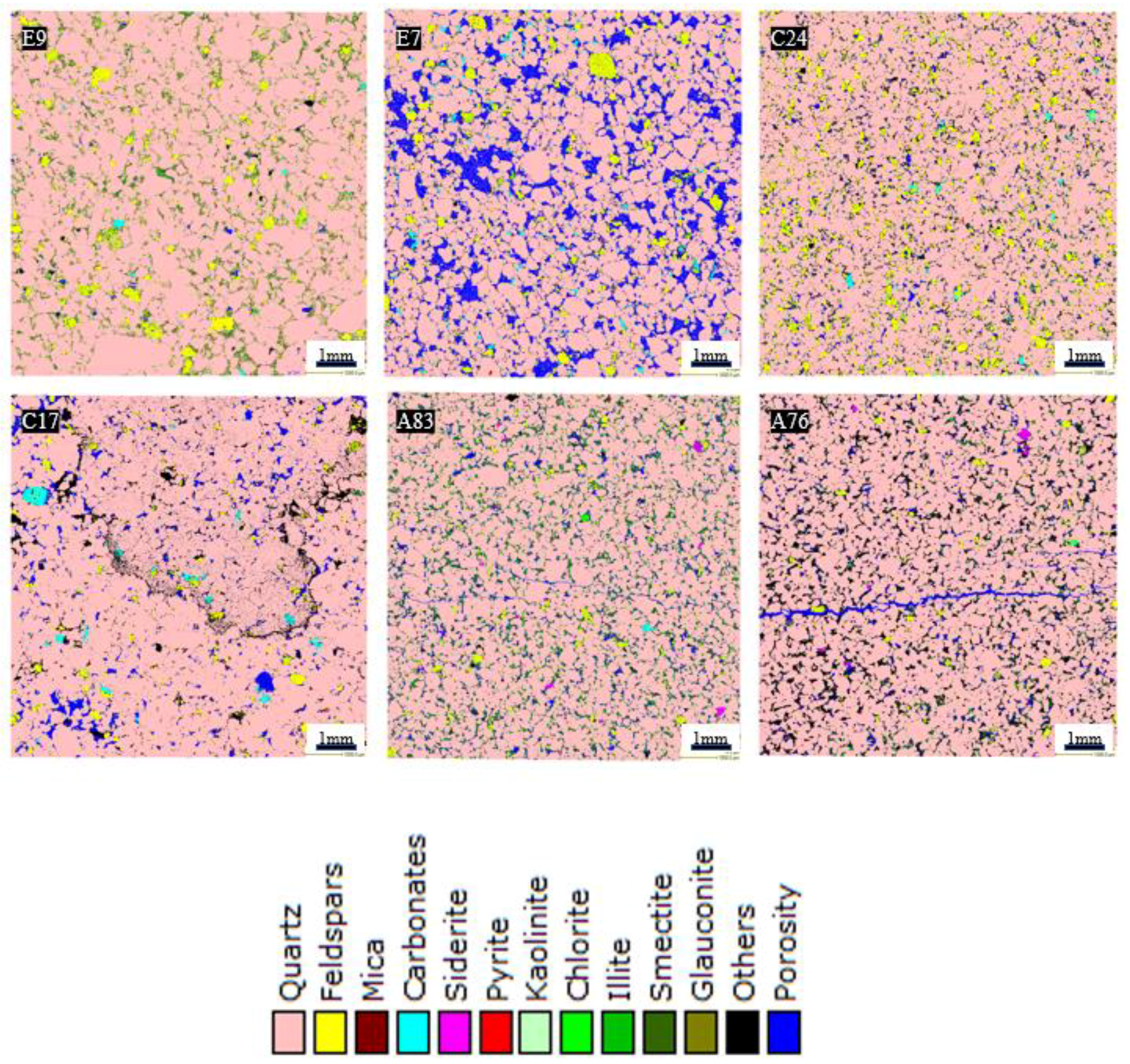
3.5. QEMSCAN Analysis

Figure 10 shows the petrographic (QEMSCAN) analysis of six thin sections representing the first porosity group (<7% porosity), while Figure 11 shows the analysis of another six sections from porosity group 2 (>7% porosity). All the facies associations are represented in the 12 subsamples. Based on quartz, feldspar, and lithic contents determined from thin-section petrography [12,13], all the samples are comprised of quartz arenite, subarkose, and sublithic arenite. The sediments’ grain sizes vary from fine, medium, and coarse, and are poorly to moderately sorted. Quartz was identified as the dominant mineral in all the FAs (Table 2). Subordinate amounts of feldspars, mica, and clay minerals were also identified. The argillaceous sandstones (Figure 10; B33) and diamictites facies (Figure 10; B25, D36, and F117) are rich in matrix content, mainly detrital illite clay mineral. Authigenic illite (Figure 11; A83 and A76), siderite (Figure 10; B25 and D33), and a minor amount of other clay minerals, including chlorite and smectite minerals, are also present in some of the lithofacies. Based on sedimentological background, the reservoir quality in porosity group 2 was generally increased by the preserved and secondary porosity, as well as fractures (e.g., Figure 11; A76), while it was diminished in group 1 by the increase of detrital matrix content (mainly illite), diagenetic siderite cement, and grain compaction (e.g., Figure 10; B16).

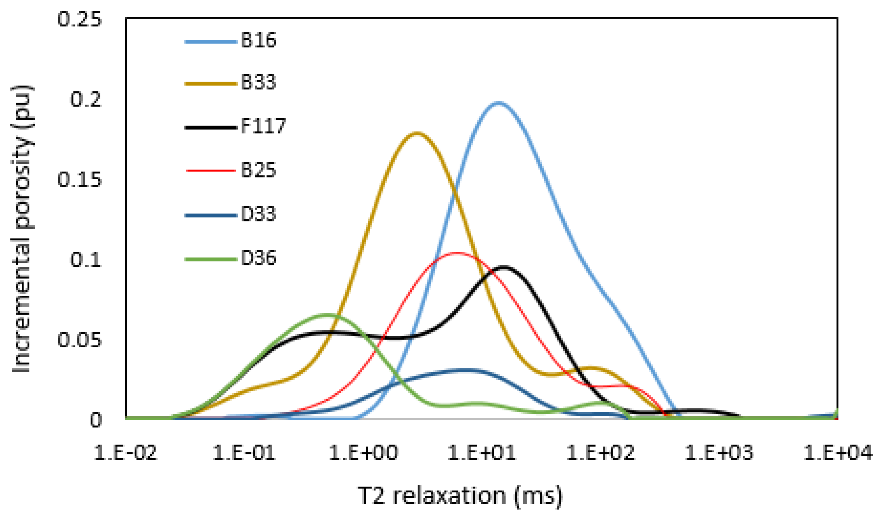
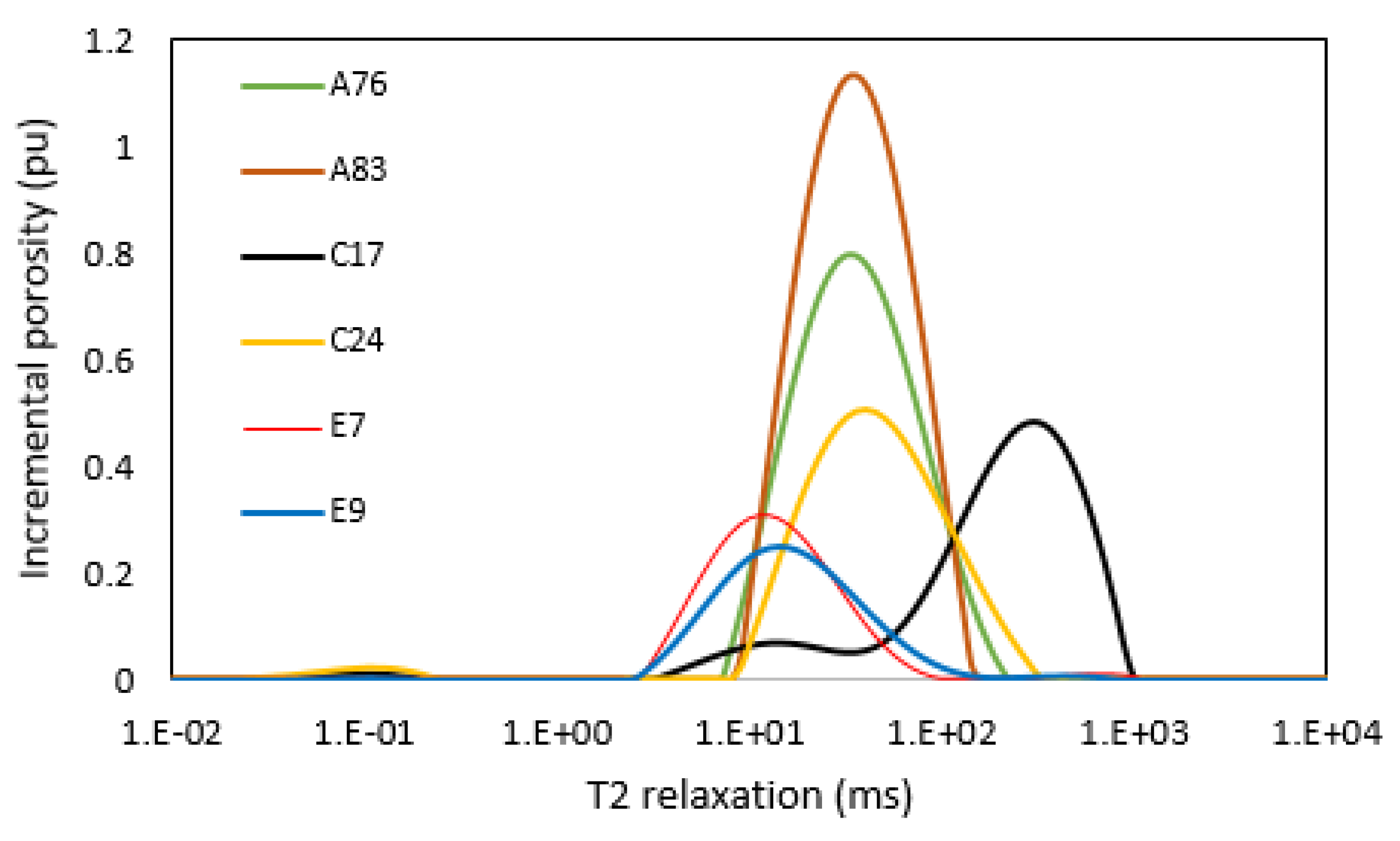
3.6. NMR T2 Distribution and Permeability

NMR measurements were also conducted on the 12 subsamples representing the two porosity groups, as shown in Figure 12 (for group 1) and Figure 13 (for group 2). The NMR T2 data show that the pore size distribution in the samples are characterized by unimodal and polymodal pore systems. The samples in group 1 mainly showed polymodal pore distribution. The pore size distribution appears to have been controlled by the proportion of clay content and the presence of fractures in the samples. As shown by their petrographic analysis, they contain a fair amount of clay minerals (Illite: 7.8%–21.44%). They are also predominantly delineated by micropores (with a T2 range of 0.01–1 ms) and macropores (with a T2 range of > 1–1000 ms), as shown in the NMR T2 curves in Figure 12. The micropore-bearing samples are dominantly matrix-rich, and they mainly represent the argillaceous sandstone and mud-rich diamictites facies. On the other hand, the samples in porosity group 2 showed a unimodal pore system (except for sample A83, which appears to be bimodal) characterized by mainly macropores with a T2 range of > 1–1000 ms (Figure 13). They contain a minor amount of clay minerals (illite: 0.95%–5.56%). The macroporosity in these samples is either due to the preserved primary porosity or secondary porosity created by the digenetic alteration of labile minerals, mainly feldspars grains, in the samples. It was also observed that the pores with a T2 range of 100–1000 ms in some of the samples may be due to the presence of microfractures (Figure 13).

3.7. NMR Porosity and Permeability

NMR porosity and pore size distribution were subsequently measured on 56 samples out of the 140 samples. A comparison made between different methods of porosity measurements, namely helium, NMR, and gravimetric porosity, reveals an acceptable match between the helium porosities and those derived from NMR and gravimetric methods (Figure 14 and Figure 15). However, it can be observed that at a porosity value above 7%, there is a scatter between all the porosity measurements. Both NMR and gravimetric porosities were measured under unconfined pressure, while helium porosity was conducted at a net confining pressure of 500 psi. Hence, the fairest comparison is that between NMR and gravimetric porosities (Figure 14). The NMR porosity and gravimetric porosity have a very good match at porosity values of 7% and below. On the other hand, there is a significant disparity between the two measurements at porosity greater than 7%. The reasons for the scatter at the 7% porosity group margin requires a closer interrogation. A closer look at the data in Figure 15 shows a better match between the gravimetric and helium porosities at this porosity range. Consequently, the mismatch could be attributed to errors in NMR measurements, particularly at porosity greater than 7%. The ability to keep the water saturation constant during gravimetric and NMR measurements dictates the level of match between the two measurement methods. Two important factors can affect the ability to sustain a constant water saturation in both measurements. These include (a) the process of wiping off excessive water from the sample surface, and (b) the duration of the porosity measurements. Gravimetric measurements take a few seconds, whereas NMR measurements require multiple scanning in order to achieve a good signal-to-noise ratio, and as such, a considerable amount of time can be expended on a single NMR measurement (an average of 10 min). During this extended time, there is a possibility of losing some of the pore water to evaporation (if the plastic wrap leaks), especially for relatively highly-porosity samples (with internal vugs, microfractures, etc.). Then, this leads to underestimated porosity values. Similarly, for these high-porosity samples, the insufficient wiping of excess water from the surface vugs can cause an overestimation of porosity. This explains why some NMR porosity values are either higher or lower than the gravimetric porosity. The QEMSCAN images of samples E7, E9, A76, A83, C17, and C24 in Figure 11 corroborates our inference. The images showed large pores, microfractures, and well-connected pores compared to the low and not well-connected pores in samples having porosity below 7% (as shown in the QEMSCAN images in Figure 10). For tighter rock samples such as those below the 7% margin, the pore water cannot be easily wiped off during the process of wiping off excessive water. Similarly, the pore water can take a much longer time than the NMR experiment time to start evaporating in the event of leakage in the plastic wrap. This explains why the NMR and gravimetric porosity have a very good match at porosity of 7% and below. It was observed that some samples in the porosity group 2 (>7%) also have a good correlation between the two measurement methods. This indicates that porosity alone may not be responsible for the scatter in this group (>7%) of samples. In order to probe this phenomenon further, high-resolution image analysis was used to investigate the pores and pore throats of samples in both groups. This is discussed in the following subsection.
NMR permeability was also estimated using the SDR model [20] and compared with laboratory measurements. The SDR equation is shown in Equation (6):
K = a T 2 L M b c
where K is permeability (mD), T 2 L M is the log mean of relaxation time (milliseconds), and is porosity (fraction). The parameters a–c are constants that can be adjusted to have a good match between NMR permeability and measured permeability. Figure 16 shows the cross-plot of the calculated NMR permeability with measured permeability for the 56 samples. The optimized model parameters that gave the best match with measured permeability are a = 14, b = 2, and c = 1, with a root mean square error (RMSE) of 1.83 and R2 value of 0.6. In Figure 17, a T2 relaxation time at a 99% sample saturation state was used instead of T 2 L M . The optimized model parameters for this case are a = 2, b = 4, and c = 2, with an RMSE value of 2.19 and an R2 value of 0.6.

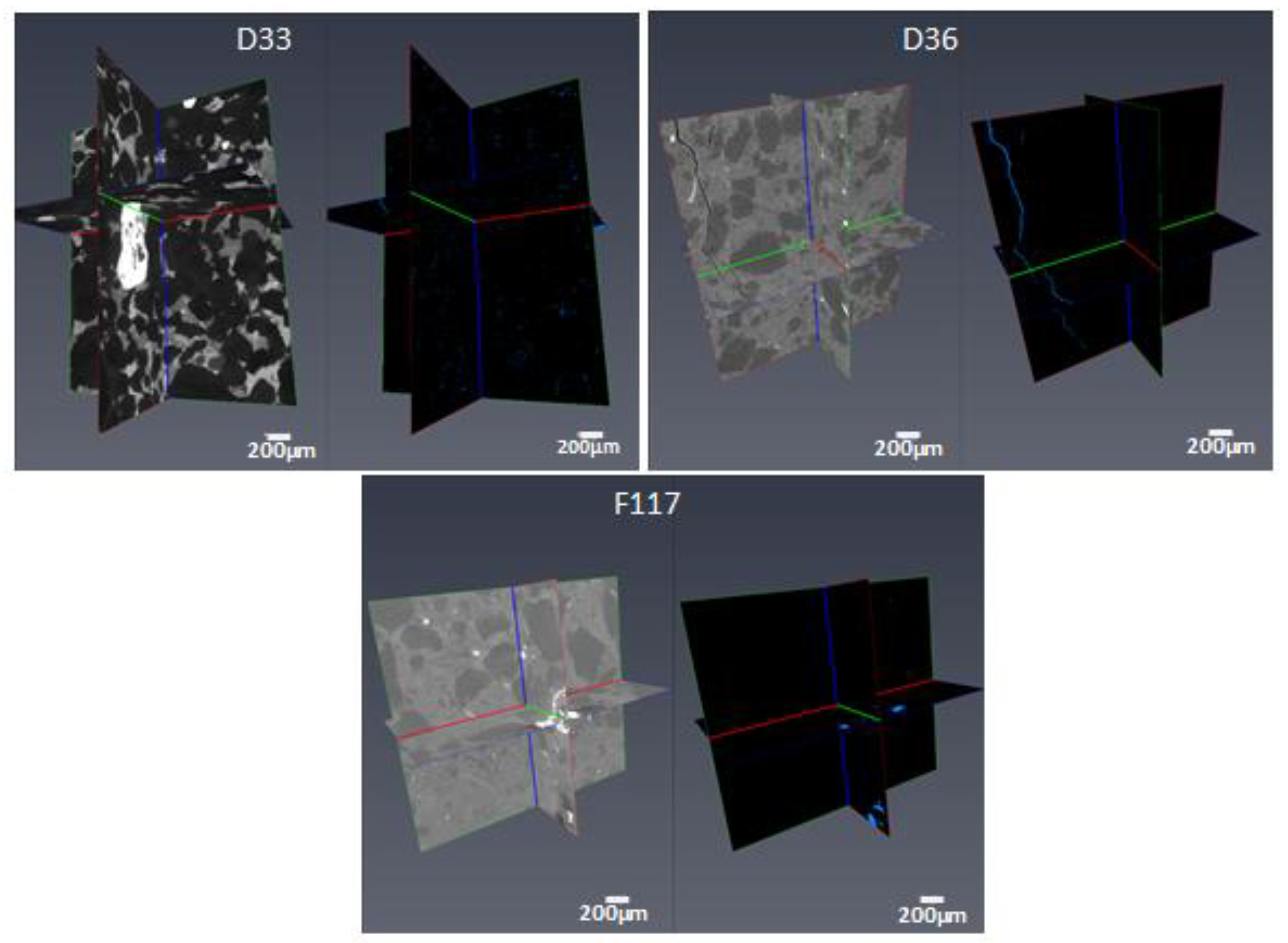
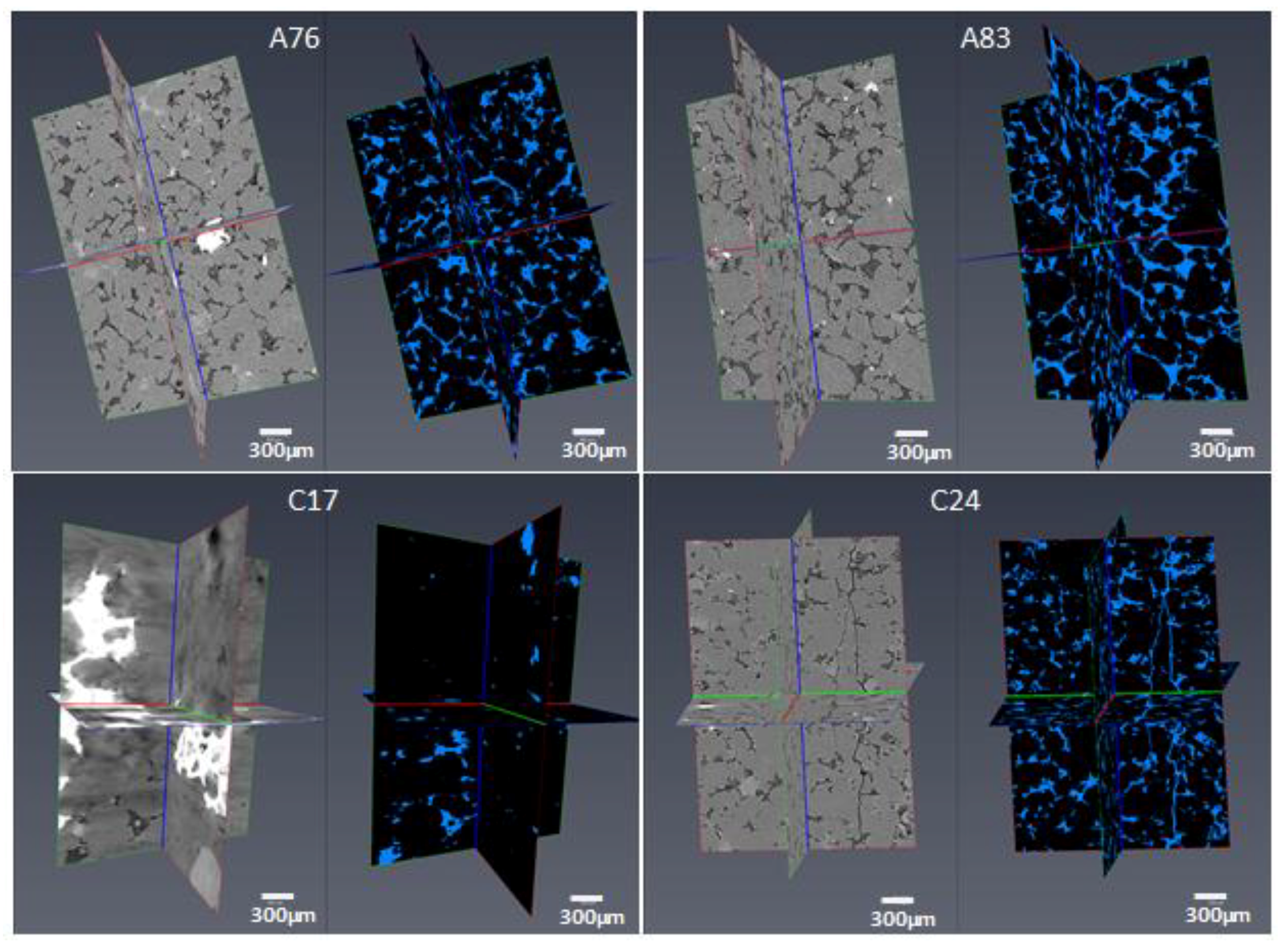
3.8. High-Resolution CT Images

QEMSCAN images do not provide enough details of samples’ pores and pore throats. Digital analysis of micro-CT images at high resolutions can elaborate more on the pore structure of these two groups of samples. In order to obtain high-resolution images, seven small rock cuttings selected from the two porosity groups were scanned at about 4-µm voxel resolution and segmented using PerGeos software. A gradient marker-based watershed segmentation was performed, and isolated pores were removed using the Axis Connectivity tool. The connected pore space was used as an input to the pore network extraction module of PerGeos software, and a pore network model was obtained for each sample showing the pores and throats. The pore network model is a spatial graph with branching or endpoints of the network labeled as pores and the connecting lines labeled as throats. The porosities computed using micro-CT analysis were found to be similar to the porosity measured using helium porosimeter (Figure 18).
Figure 19 and Figure 20 show the segmented 2D images for group 1 and group 2, respectively. We could not carry out detailed digital analysis on some of the selected samples (especially the samples with poor connectivity) because of limitations in equipment resolution, which made it impossible to resolve smaller pores. Coincidentally, these poor connectivity samples have an excellent match between the gravimetric and NMR porosity measurements.
The high-resolution images show that the porosity group 1 samples have tight and poorly connected pores compared to the porosity group 2 samples, which have much better connectivity. These CT images conform to the QEMSCAN images and corroborate our inference regarding the disparity in the correlation between gravimetric and NMR porosities. A pore network model of selected samples from both porosity groups revealed the pore throat and pore size distribution from both groups. Interestingly, samples with a good match between gravimetric and NMR porosity have tighter pore throats with a pore throat size in the range of 2–20 µm (Figure 21), while samples that matched poorly between the two porosity methods have bigger pore throats or better connectivity, with pore throat sizes ranging between 2 and 50 µm (Figure 22). Figure 23 shows the pore network model of sample C24 (with a pore throat size range of 2–20 µm) and sample A83 (with pore throat sizes ranging from 2 to 50 µm). One may be tempted to speculate that pore throat sizes in excess of 20 µm may be responsible for the scatter in the porosity cross-plots, since they allow the water in the pores to be drained or lost during NMR measurements. Sample C24 has porosity above the 7% cut-off, but the pore throat size is similar to the samples in group 1 (<7%). This suggests that the scattering observed in the porosity cross-plots is not due to porosity values alone but also due to the connectivity of the pores. This also explains why some samples in group 2 also showed a good match between the two porosity measurements even when their porosity values are above the 7% cut-off.

3.9. Formation Resistivity and Cementation Factors

Archie defined the ratio of the resistivity of a rock at 100% water saturation ( R o ) to the resistivity of the water ( R w ) as the formation resistivity factor (or formation factor) given by Equation (7):
F F = R o R w
The formation factor (FF) is dependent on various properties of the rock such as the porosity, degree of cementation, and clay content. For a clean sand and limestone, where clay is absent, FF remains constant as brine resistivity changes. For a shaly sand (containing clay), FF will decrease as brine resistivity increase and vice versa. This is because the clay content in the rock also serves as a conductor, which does not allow R o to increase proportionally with R w . This clay effect depends on the amount, type, and distribution of the clay in the rock. The simplest relationship between FF and porosity ( ) is:
F F = 1
Equation (8) was derived with the assumption that the rock matrix is embedded with straight and parallel capillaries. Different researchers developed different forms of Equation (8), as shown in Table 3, Equations (9)–(13). These models to a large extent incorporate a tortuosity factor ( τ ) in the relationship between FF and porosity. The tortuosity factor is a measure of the departure of a porous medium from the ideal system made of straight and parallel capillaries.
FF is also dependent on the degree of cementation of the rock. The degree of cementation depends on the cementing material (i.e., silica, calcite, or clay), amount of cement, and distribution of the cement materials. The higher the cementation, the lower the porosity, and then the higher the FF. Archie derived the relationship between FF, porosity, and cementation factor (m), as shown in Equation (14). The cementation factor or porosity exponent (m) is a function of the large number of factors such as the type, shape, and distribution of pores; packing and sorting of grains; tortuosity; presence of clay; compaction due to overburden stress, etc. Humble modified Equation (14) to include another constant (a), which is also dependent on the rock type. This constant (a) is an empirical constant, and it is sometimes referred to as tortuosity factor or cementation intercept. A value of “a” other than 1 compensates for variation in the FF– relationship due to differences in the compaction, pore structure, and grain size [26].
F F = 1 m
F F = a m
The cementation factor often ranges between 1.3 for loose unconsolidated sand to as high as 3 in carbonates [15,16].
In Figure 24, the formation factors of 56 samples are plotted against their porosity values. Four pole electrical resistivity measurements were conducted at a 100% water saturation state for 56 subsamples. The samples were saturated with formation brine and subjected to a net-confining pressure of 500 psi and room temperature of 25 °C. The measured formation factor and porosity were fitted with Equation (14) using m values of 1.5. If we allow “a” value other than one (1), the tortuosity factor (“a”) estimated as the intercept of the slope at 100% porosity was found to be 5.14 with an estimated cementation factor 0.98 (from the slope of the plot). Tortuosity was also calculated for these samples using the equations provided in Table 3. The tortuosity range based on each equation is given in Table 4. The tortuosity values for the 12 subsamples are listed in Table 5. In addition, Table 5 also contains a list of the different petrophysical measurements conducted on the 12 samples that represent the six wells as well as the different hydraulic flow units.

4. Conclusions

An integrated petrophysical and petrological study was conducted on 140 core plugs from a Saudi Arabian tight gas reservoir. A detailed suite of experiments was conducted using a variety of analytical tools such as a helium porosity–permeability meter, NMR, electrical resistivity, micro-CT imaging, thin section, and QEMSCAN. We found that two distinct groups of porosity occur in the studied reservoir and that each group responded differently to the laboratory methods of porosity measurements. In order to probe this observation further, a gradient marker-based watershed segmentation together with digital rock physics computation were used to generate the pore network models, pores, and pore size distribution of representative samples. Then, we speculated how the pore character of the tight formation affected methods of porosity measurements in the laboratory. Then, the following specific conclusions were made from this study.
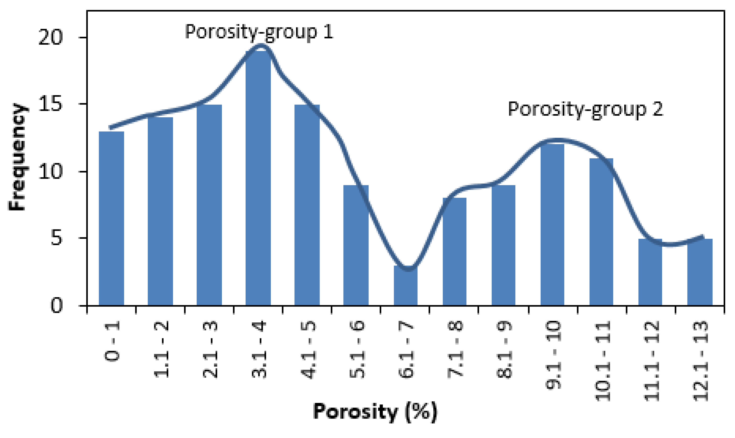
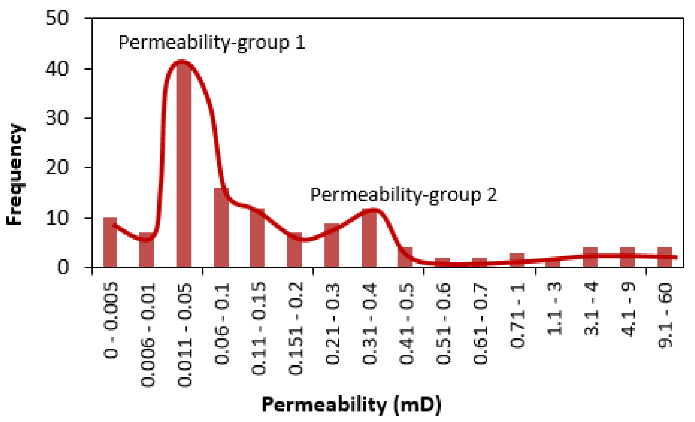
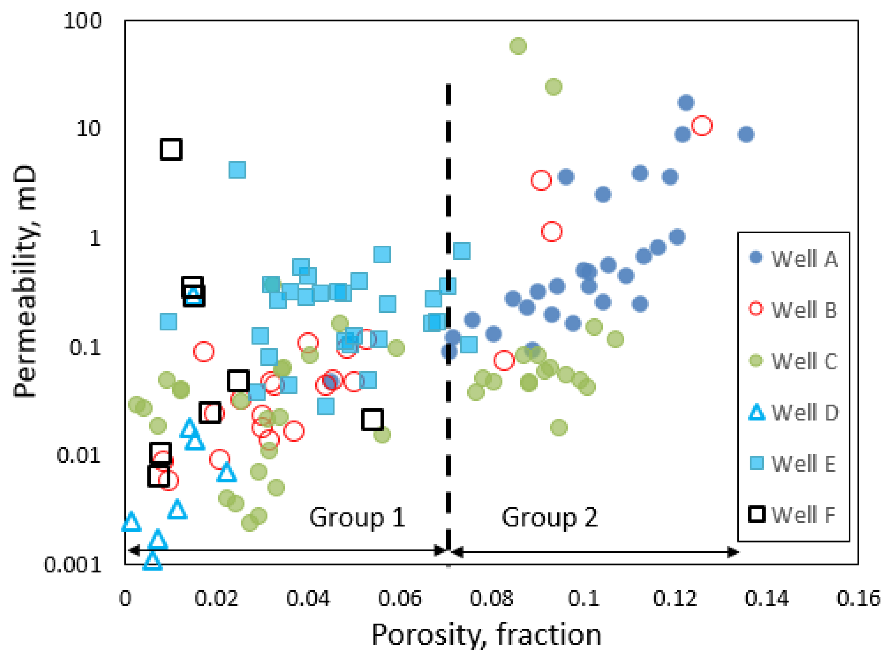
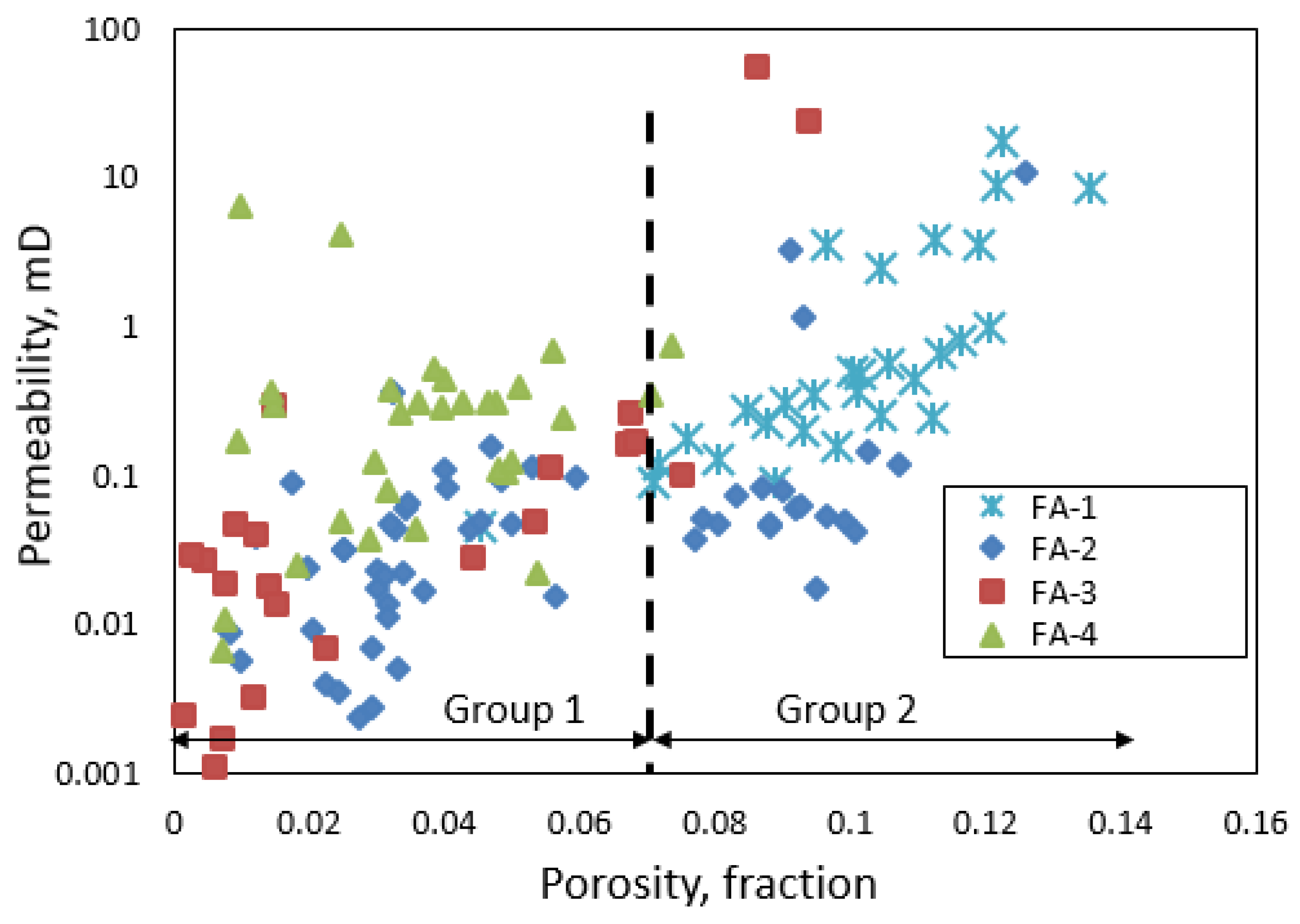
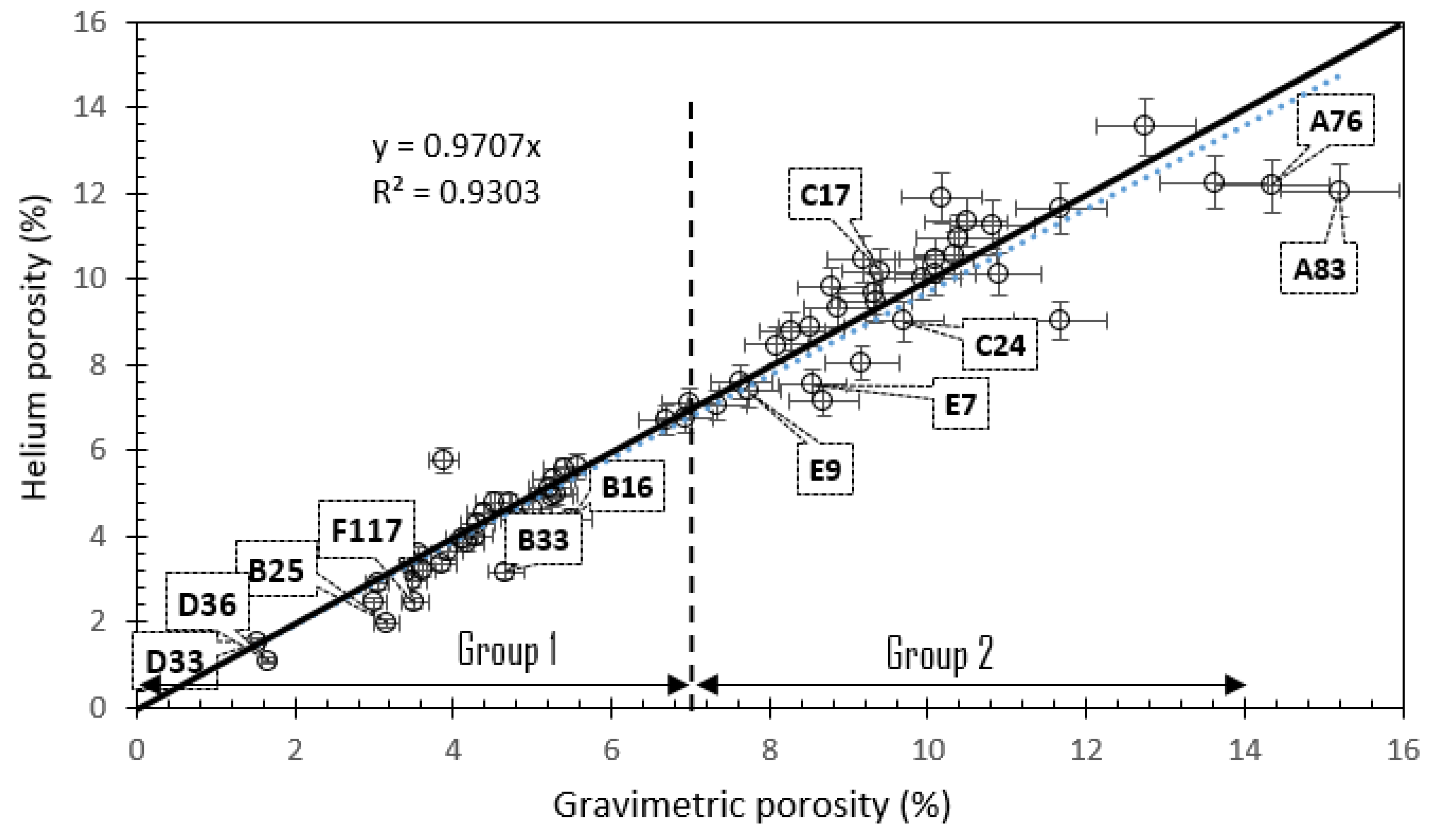
  • Our analysis identified two major porosity groups of rock samples. One group is characterized by porosity values less than 7% while the second group has porosity values above 7%. There is a generally a good agreement between different methods of porosity measurements in samples with <7% porosity compared to samples with >7% porosity values.
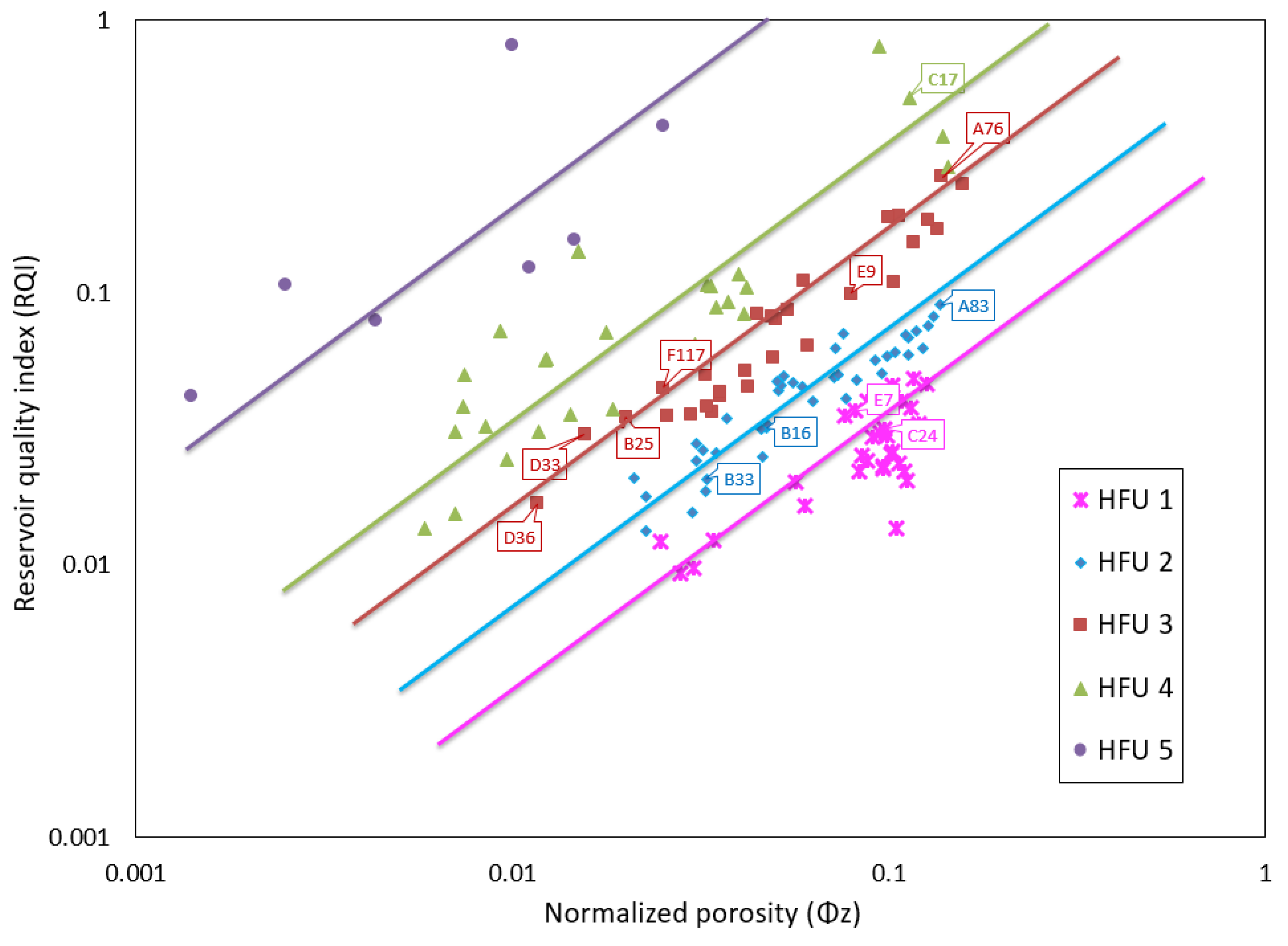
  • Rock typing using the flow zone indicator (FZI) identified five hydraulic flow units (HFUs). Each of the HFUs has reservoir rocks with porosity values that fall within both groups of porosity.
  • Petrographic analysis revealed that the low-porosity samples have a significant amount of clay (mainly illite). However, quartz was identified as the dominant mineral in all the rock samples while subordinate amounts of feldspars, mica, and clay minerals were also identified.
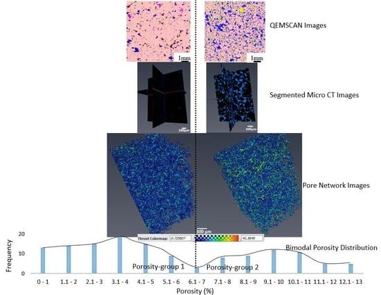
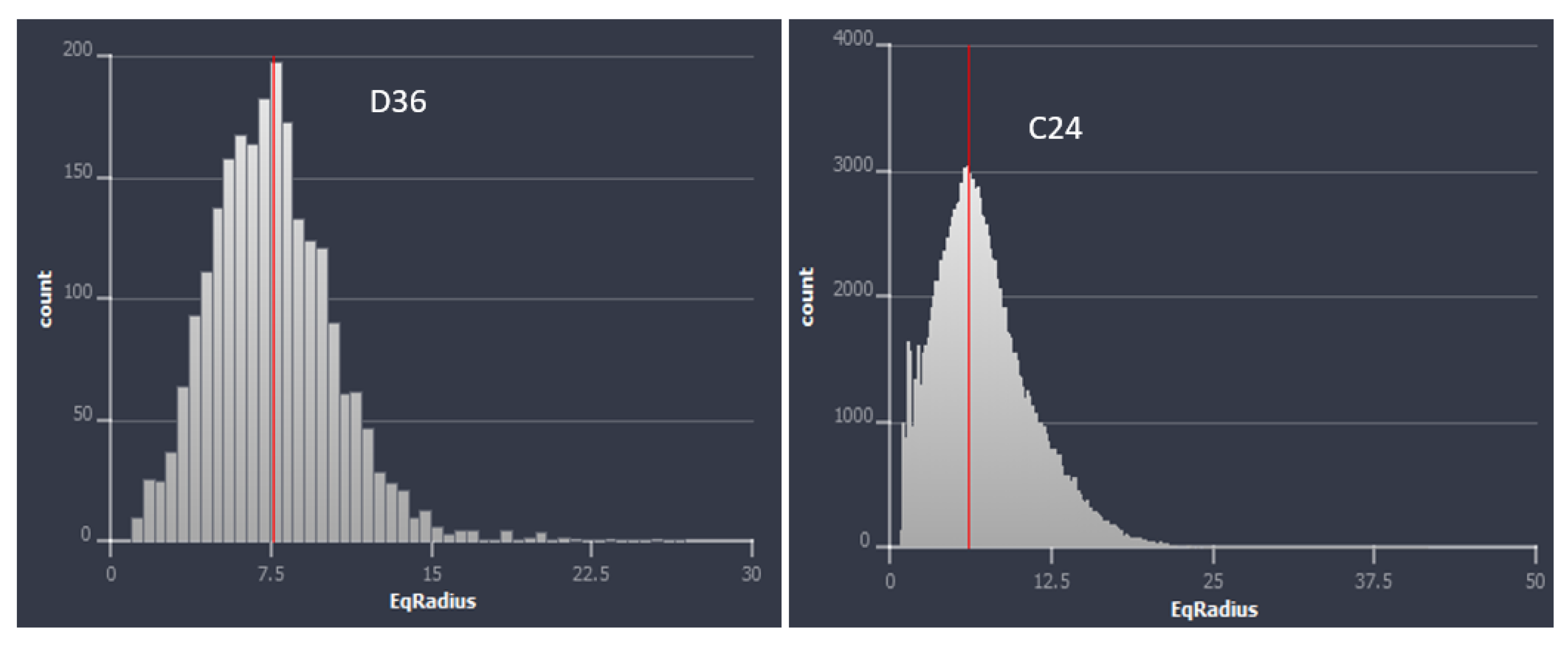
  • NMR analysis showed that the group 1 samples are dominated by micropores, while the group 2 samples are dominated by macropores. Group 1 samples apparently showed a polymodal pore system, while the samples in group 2 generally showed unimodal pore distribution.
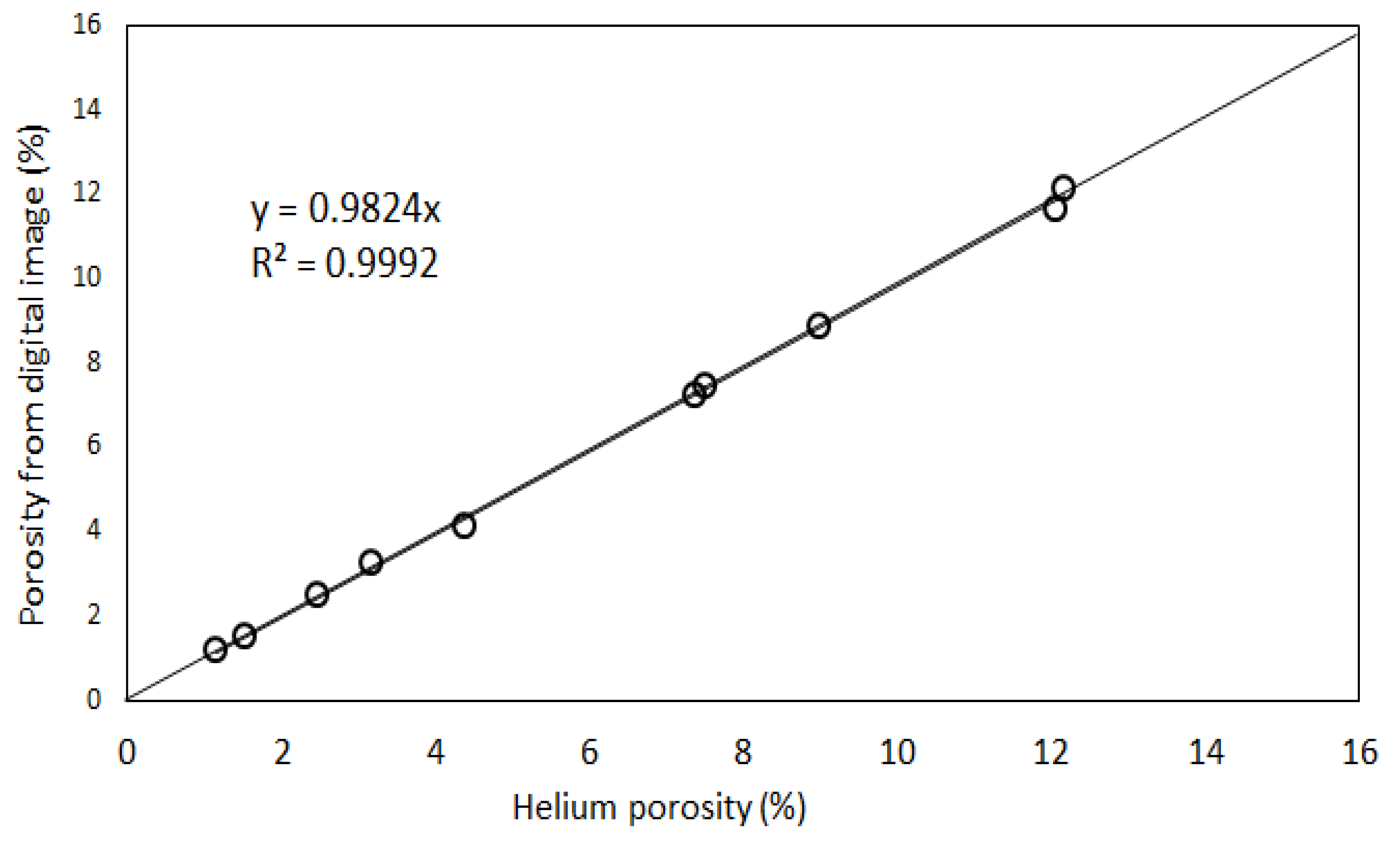
  • High-resolution micro-CT images showed that pore throat size plays a very important role in the NMR porosity measurements, and may be responsible for the poor correlation between NMR porosity and gravimetric porosity in the group 2 samples (>7%).
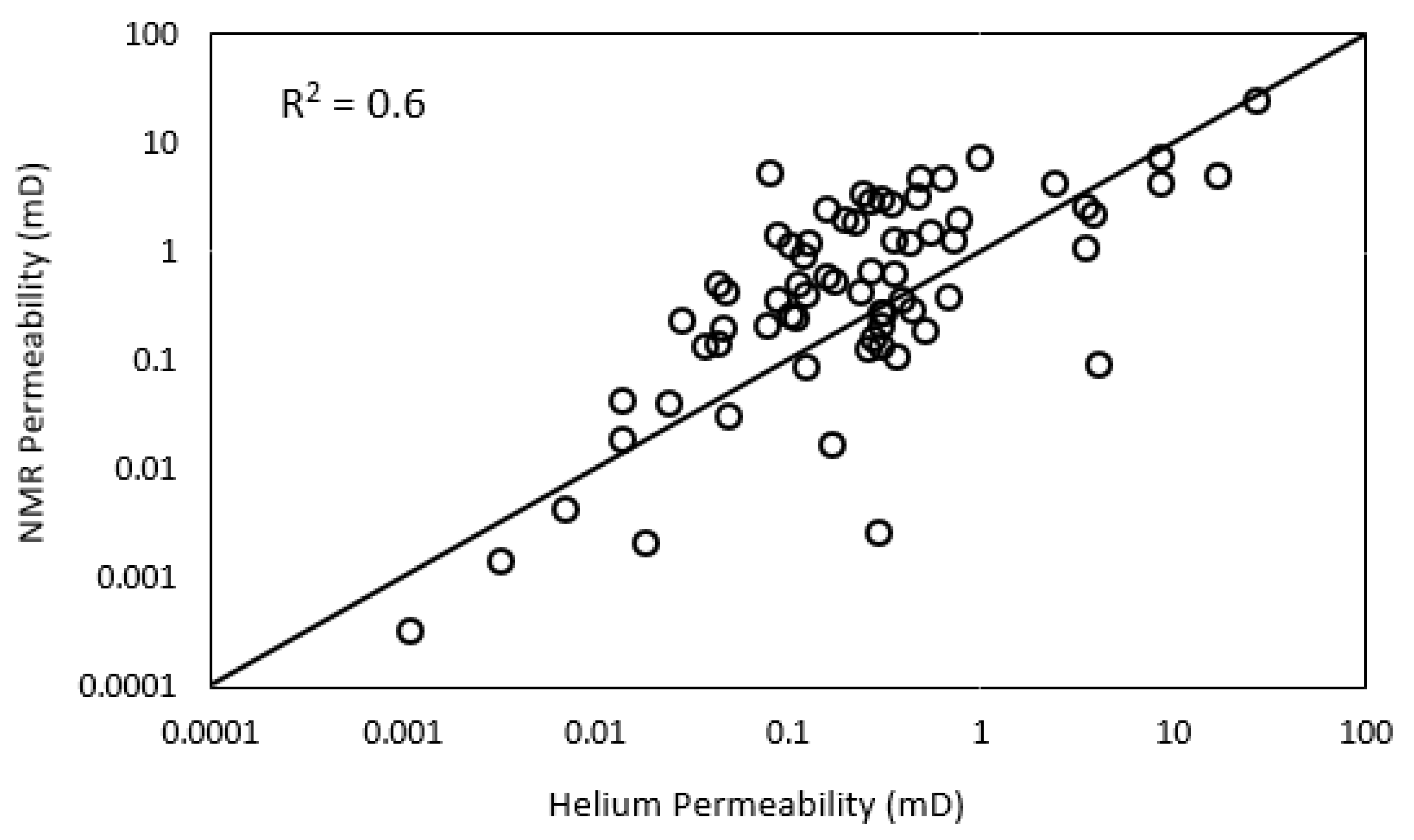
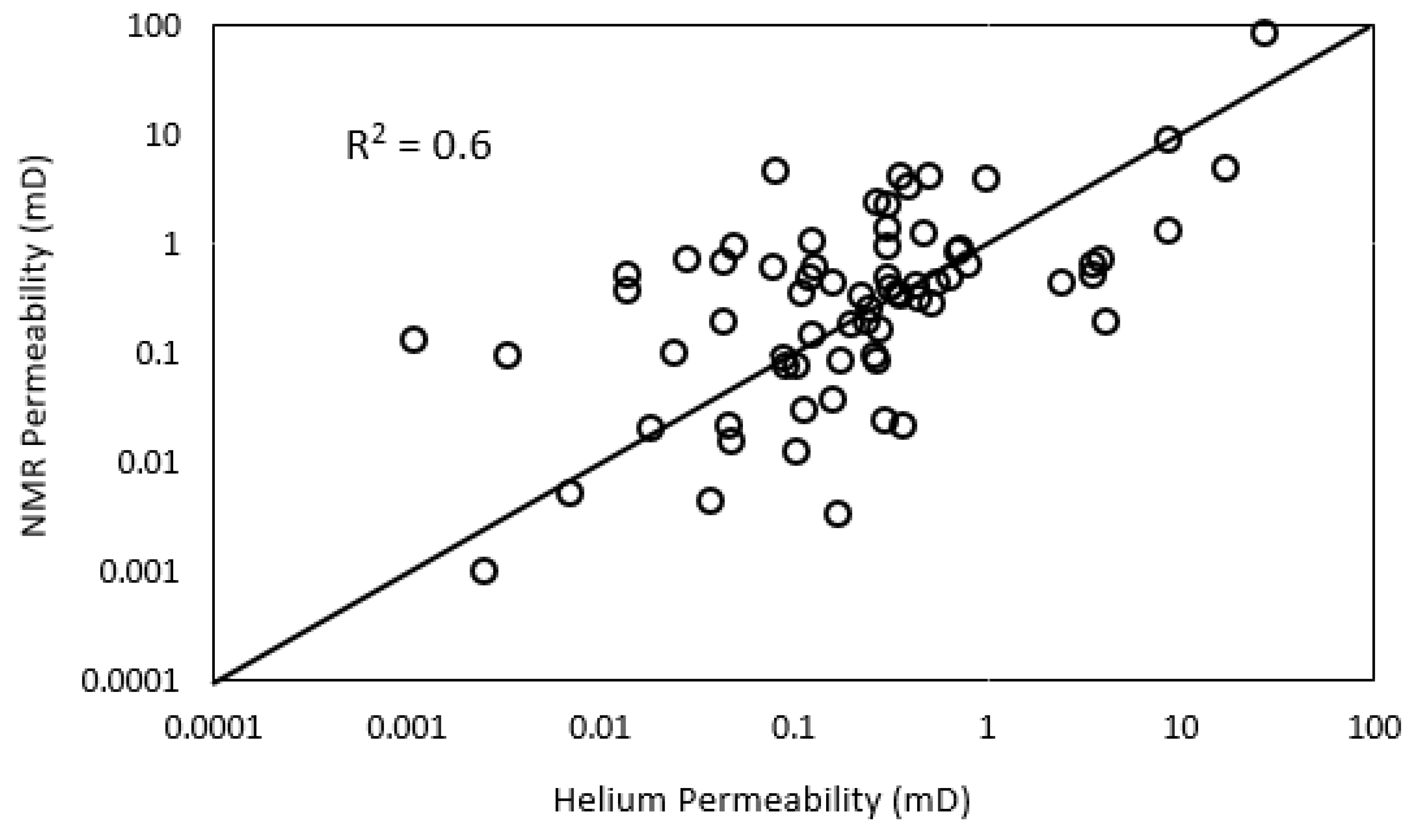
  • NMR-estimated permeability in tight sandstones shows fair correlation with helium permeability with an R2 of 0.6 and RMSE of 1.8.
  • Electrical resistivity measurements showed that the tight sand samples have a cementation factor of 1.5, when the laboratory measurements are fitted with the Archie model. When a value of tortuosity factor other than 1 is allowed, the cementation factor is about 1 and the tortuosity factor is 5.14. Electrical tortuosity values computed using various empirical models range between 1.2 and 9.6.

Author Contributions

Conceptualization, A.R.A. and L.B.; Methodology, A.R.A. and L.B.; Software, S.R.H. and A.A.; Formal analysis, A.R.A., L.B., R.S.B., S.R.H., and A.A.; Investigation, A.R.A., L.B., and R.S.B.; Resources, A.R.A. and L.B.; Data curation, R.S.B.; Writing—original draft preparation, A.R.A.; Writing—review and editing, L.B.; Supervision, A.R.A. and L.B.; Project administration, L.B. and A.A.; Funding acquisition, L.B.

Funding

This research was funded by King Abdulaziz City for Science and Technology as part of the National Science, Technology, and Innovation Plan (NSTIP Project # 14-OIL468-04) through the Science and Technology Unit at KFUPM.

Acknowledgments

We duly acknowledge the Ministry of Energy, Industry and Mineral Resources, Saudi Arabia for providing the cores and plug samples used in this study. The contribution by Late Ali Sahin is also highly appreciated. We thank the anonymous reviewers for their critical and constructive review.

Conflicts of Interest

The authors declare no conflict of interest.

References

  1. Saudi Aramco Unconventional Gas: A Growing Resource. Available online: https://www.jobsataramco.eu/people-projects/unconventional-gas-growing-resource (accessed on 8 June 2019).
  2. Weeden, S. Saudi Arabia Gears Up For Unconventional Gas Exploration. Available online: https://www.hartenergy.com/exclusives/saudi-arabia-gears-unconventional-gas-exploration-19011#p=full (accessed on 8 June 2019).
  3. Shehata, A.; Tps, A.U.C.; Aly, A.; Schlumberger, A.U.C.; Ramsey, L.; Tgcoe, S. Overview of Tight Gas Field Development in the Middle East and North Africa Region. In Proceedings of the North Africa Technical Conference and Exhibition, Cairo, Egypt, 14–17 February 2010. [Google Scholar]
  4. Luffel, D.L.; Howard, W.E. Reliability of Laboratory Measurement of Porosity in Tight Gas Sands. In Proceedings of the Low Permeability Reservoirs Symposium, Denver, Colorado, 18–19 May 1987. [Google Scholar]
  5. Sondergeld, C.H.; Newsham, K.E.; Comisky, J.T.; Rice, M.C.; Rai, C.S. Petrophysical considerations in evaluating and producing shale gas resources. In Proceedings of the SPE Unconventional Gas Conference; Society of Petroleum Engineers, Pittsburgh, PA, USA, 23–25 February 2010. [Google Scholar]
  6. Song, L.; Warner, T.; Carr, T. An efficient, consistent, and trackable method to quantify organic matter–hosted porosity from ion-milled scanning electron microscope images of mudrock gas reservoirs. Am. Assoc. Pet. Geol. Bull. 2019, 103, 1473–1492. [Google Scholar] [CrossRef]
  7. Bush, D.C.; Jenkins, R.E. Proper Hydration of Clays for Rock Property Determinations. J. Pet. Technol. 1970, 22, 800–804. [Google Scholar] [CrossRef]
  8. Sullivan, M.; Song, L. Briggs colour cubing of spectral gamma ray—A novel technique for easier stratigraphic correlation and rock typing. In Proceedings of the SPWLA 58th Annual Logging Symposium, Oklahoma City, OK, USA, 17–21 June 2017. [Google Scholar]
  9. Morrow, N.R.; Cather, M.E.; Buckley, J.S.; Dandge, V. Effects of Drying on Absolute and Relative Permeabilities of Low-Permeability Gas Sands. In Proceedings of the Low Permeability Reservoirs Symposium, Denver, Colorado, 15–17 April 1991. [Google Scholar]
  10. Laboun, A.A. Regional tectonic and megadepositional cycles of the Paleozoic of northwestern and central Saudi Arabia. Arab. J. Geosci. 2013, 6, 971–984. [Google Scholar] [CrossRef]
  11. Al-Harbi, O.A.; Khan, M.M. Source and origin of glacial paleovalley-fill sediments (Upper Ordovician) of Sarah Formation in central Saudi Arabia. Arab. J. Geosci. 2011, 4, 825–835. [Google Scholar] [CrossRef]
  12. Alqubalee, A.; Abdullatif, O.; Babalola, L.; Makkawi, M. Characteristics of Paleozoic tight gas sandstone reservoir: integration of lithofacies, paleoenvironments, and spectral gamma-ray analyses, Rub’ al Khali Basin, Saudi Arabia. Arab. J. Geosci. 2019, 12, 344. [Google Scholar] [CrossRef]
  13. Alqubalee, A.; Babalola, L.; Abdullatif, O.; Makkawi, M. Factors Controlling Reservoir Quality of a Paleozoic Tight Sandstone, Rub’ al Khali Basin, Saudi Arabia. Arab. J. Sci. Eng. 2019, 1–19. [Google Scholar] [CrossRef]
  14. Klinkenberg, L.J. The permeability of porous media to liquids and gases. In Proceedings of the Drilling and Production Practice, New York, NY, USA, 1 January 1941. [Google Scholar]
  15. Ayling, B.; Rose, P.; Petty, S.; Zemach, E.; Drakos, P. QEMSCAN® Quantitative evaluation of minerals by scanning electron microscopy: capability and application to fracture characterization in geothermal systems. In Proceedings of the Thirty-Eighth Workshop on Geothermal Reservoir Engineering, Stanford University, Stanford, CA, USA, 30 January–1 February 2012; p. 11. [Google Scholar]
  16. Gottlieb, P.; Wilkie, G.; Sutherland, D.; Ho-Tun, E.; Suthers, S.; Perera, K.; Jenkins, B.; Spencer, S.; Butcher, A.; Rayner, J. Using quantitative electron microscopy for process mineralogy applications. JOM 2000, 52, 24–25. [Google Scholar] [CrossRef]
  17. Qian, G.; Li, Y.; Gerson, A.R. Applications of surface analytical techniques in Earth Sciences. Surf. Sci. Rep. 2015, 70, 86–133. [Google Scholar] [CrossRef]
  18. Elster, A. MRIQuestion: T2 Relaxation Definition. Available online: http://mriquestions.com/what-is-t2.html (accessed on 8 October 2019).
  19. Amaefule, J.O.; Kersey, D.G.; Marschall, D.M.; Powell, J.D.; Valencia, L.E.; Keelan, D.K. Reservoir Description: A Practical Synergistic Engineering and Geological Approach Based on Analysis of Core Data. In Proceedings of the SPE Annual Technical Conference and Exhibition, Houston, TX, USA, 2–5 October 1988. [Google Scholar]
  20. Al-Ajmi, F.; Holditch, S. NMR Permeability Calibration using a Non-Parametric Algorithm and Data from a Formation in Central Arabia. In Proceedings of the SPE Middle East Oil Show, Manama, Bahrain, 17–20 March 2001. [Google Scholar]
  21. Winsauer, W.O.; Shearin, H.M.; Winsauer, W.O.; Shearin, H.M., Jr.; Masson, P.H.; Williams, M. Resistivity of Brine-Saturated Sands in Relation to Pore Geometry. Am. Assoc. Pet. Geol. Bull. 1952, 36, 253–277. [Google Scholar]
  22. Wyllie, M.R.J.; Spangler, M.B. Application of Electrical Resistivity Measurements to Problem of Fluid Flow in Porous Media. Am. Assoc. Pet. Geol. Bull. 1952, 36, 359–403. [Google Scholar]
  23. Faris, S.R.; Gournay, L.S.; Lipson, L.B.; Webb, T.S. Verification of Tortuosity Equations: GEOLOGICAL NOTES. Am. Assoc. Pet. Geol. Bull. 1954, 38, 2226–2232. [Google Scholar]
  24. Pirson, S.J. Geological Well Log Analysis; Gulf Publishing Co.: Houston, TX, USA, 1983. [Google Scholar]
  25. Cornell, D.; Katz, D.L. Flow of Gases through Consolidated Porous Media. Ind. Eng. Chem. 1953, 45, 2145–2152. [Google Scholar] [CrossRef]
  26. McPhee, C.; Reed, J.; Zubizarreta, I. Core Analysis: A Best Practice Guide; Elsevier: Amsterdam, The Netherlands, 2015. [Google Scholar]
Figure 1. (A) Surface geological map of the Arabian Plate, (B) gravity map showing the basement topography underneath the study area.
Energies 12 04302 g001
Figure 2. Core stratigraphic columns showing the different facies associations for all wells: FA1: fluvial, FA2: glaciolacustrine delta, FA3: subglacial, and FA4: glaciofluvial outwash facies.
Energies 12 04302 g002
Figure 3. Porosity distribution of 140 rock samples extracted from six wells.
Energies 12 04302 g003
Figure 4. Permeability distribution of 140 rock samples extracted from six wells.
Energies 12 04302 g004
Figure 5. Cross-plot of helium porosity and helium permeability of 140 rock samples classified based on the wells from which they were extracted.
Energies 12 04302 g005
Figure 6. Photomicrographs for microfacies observed in the analyzed samples. (A) Heterogenous patterns of grain compactions, (B) interparticle porosity associated with grain compaction, (C) intraparticle porosity due grains dissolution, (D) fractures associated with grain compactions, (E) authigenic pore-filling illite, (F) pore-filling anhydrite and barite cement.
Energies 12 04302 g006
Figure 7. Cross-plot of helium porosity and helium permeability of 140 rock samples classified based on facies associations.
Energies 12 04302 g007
Figure 8. Hydraulic flow units of the reservoir identified from 140 rock samples from six wells.
Energies 12 04302 g008
Figure 9. Cross-plot of helium porosity and helium permeability of 140 rock samples classified based on hydraulic flow units.
Energies 12 04302 g009
Figure 10. Quantitative evaluation of minerals by scanning electron microscope (QEMSCAN) images of samples in porosity-group 1 (<7% porosity). The color codes for different minerals and pores are shown in the legend.
Energies 12 04302 g010
Figure 11. QEMSCAN images of samples in porosity group 2 (>7% porosity). The color codes for different minerals and pores are shown in the legend.
Energies 12 04302 g011
Figure 12. Distribution of NMR T2 relaxation for subsamples in porosity group 1 (<7%).
Energies 12 04302 g012
Figure 13. Distribution of NMR T2 relaxation for subsamples in porosity group 2 (>7%).
Energies 12 04302 g013
Figure 14. Cross-plot of NMR porosity and gravimetric porosity for 56 subsamples.
Energies 12 04302 g014
Figure 15. Cross-plot of helium porosity and gravimetric porosity for 56 subsamples.
Energies 12 04302 g015
Figure 16. NMR-derived permeability versus core-measured permeability using T 2 L M .
Energies 12 04302 g016
Figure 17. NMR-derived permeability versus core-measured permeability using T 2 at 99% water saturation.
Energies 12 04302 g017
Figure 18. Porosity computed from digital image versus measured porosity.
Energies 12 04302 g018
Figure 19. High-resolution µCT images and their segmentations for samples in group 1 (<7% porosity). CT images taken at 3-µm resolution.
Energies 12 04302 g019
Figure 20. High-resolution µCT images and their segmentation for samples in group 2 (>7% porosity). CT images taken at 4-µm resolution.
Energies 12 04302 g020
Figure 21. Pore throat size distribution in the range of 1–20 µm. On the y-axis is the count (frequency) and the x-axis is the corresponding equivalent radii (EqRadius in µm) of the pore throats.
Energies 12 04302 g021
Figure 22. Pore throat size distribution in the range of 1–50 µm. On the y-axis is the count (frequency) and the x-axis is the corresponding equivalent radii (EqRadius in µm) of the pore throats.
Energies 12 04302 g022
Figure 23. Pore network model for samples C24 and A83. The color legend represents the pore and throats sizes, where dark blue represents small pores and throats, and red represents big pores and throats.
Energies 12 04302 g023
Figure 24. Formation resistivity factor versus porosity for 56 subsamples.
Energies 12 04302 g024
Table 1. Properties of brine (B: boron, Ba: barium, BCl: chloride, Br: bromide, Ca: calcium, EC: electrical conductivity, Fe: iron, HCO3: bicarbonate, K: potassium, Mg: magnesium, Mn: manganese, Na: sodium, Si: silicon, SO4: sulfate, Sr: stontium, TPH: total petroleum hydrocarbon, Zn: zinc).
ComponentsRange
pH4.62–6.6
EC, mmho/cm (25 °C)96–534
Total Solids (mg/L)103,250–369,200
Density (g/mL)1.088–1.264
Cl (mg/L)46,981–185,596
Br (mg/L)411–1492
SO4 (mg/L)137–1039
HCO3(mgL)<1.0
B (mg/L)25.16–43.56
Ba(mg/L)311–1275
Ca (mg/L)16,315–54,500
Fe(mg/L)695–66,700
K(mg/L)971–2870
Mg (mg/L)568–1350
Mn (mg/L)48.74–221.24
Na (mg/L)16,012–159,575
Si (mg/L)10.13–18.46
Sr (mg/L)272–1336
Zn (mg/L)92.38–188.63
TPH (mg/L)1.51–1346.75
Table 2. Mineralogy compositions of the samples in each of the facies.
Sample IDSilicates (%)Carbonates (%)PyriteClay (%)OthersFA
QuartzFeldsparsMicaCalciteSideriteKaoliniteChloriteIlliteSmectiteGlauconite
B1690.660.043.210.010.550.210.010.000.950.000.001.38FA2
B2575.321.453.060.0113.500.060.020.124.070.000.020.39FA3
B3375.123.109.270.011.760.050.030.117.810.000.010.49FA2
D3364.451.501.600.0321.210.100.010.211.130.000.038.44FA4
D3657.415.0313.160.070.000.170.130.6821.430.020.110.70FA3
F11767.448.914.130.050.260.150.030.4816.040.070.041.63FA3
A8380.891.602.230.050.260.020.230.117.820.020.011.45FA1
C2479.197.562.190.330.000.030.020.013.840.020.003.09FA2
E773.933.651.750.820.000.010.020.222.060.040.060.34FA4
E986.153.853.090.140.000.030.070.185.460.030.030.34FA4
A7680.931.130.830.020.250.030.040.062.380.000.0010.38FA1
C1785.152.051.340.720.000.020.010.000.900.010.005.29FA2
Table 3. Different electrical tortuosity models.
AuthorsTortuosity ModelEquation #
Winsauer et al. [21] τ 2 = ( F F × ) 1.2 (9)
Wyllie and Spangler [22] τ = ( F F × ) 2 (10)
Faris et al. [23] τ 2 = ( F F × ) 1.41 (11)
Pirson [24] τ 2 = F F × (12)
Cornell and Katz [25] τ = F F × (13)
Table 4. Tortuosity range for 56 subsamples using different electrical tortuosity models.
Tortuosity ModelTortuosity (τ)
Winsauer et al. [21]1.28–3.89
Wyllie and Spangler [22]2.28–92.55
Faris et al. [23]1.34–4.93
Pirson [24]1.23–3.1
Cornell and Katz [25]1.51–9.62
Table 5. Summary of measured petrophysical properties on 12 subsamples representing six wells and the different hydraulic flow units. FZI: flow zone indicator, RQI: reservoir quality index.
Sample IDHe-Porosity %NMR PorosityPermeability (mD)RQI (µm)FZI (µm)Formation factor (FF)Tortuosity (τ) *KNMR (mD)
D361.151.40.00330.0168220137.21.510.0967
D331.530.90.0140.030036100238.83.650.5224
B251.972.80.0240.034772100--0.0976
F1172.463.70.050.044759100376.739.250.9415
B333.174.90.0140.0207144--0.3646
B164.395.10.0440.0314634--0.6781
E97.374.60.7380.0993492064.054.720.8955
E77.523.30.1030.0367482.561.724.640.075
C2499.20.0810.0298442.5--4.5309
C1710.188.527.870.51959110,000--82.9
A8312.0511.20.990.0899974--3.9619
A7612.1712.98.8440.26772410037.294.548.7779
* Tortuosity based on Cornell and Katz [25] Equation (13). Electrical resistivity was not measured on some samples because of the small sample diameter.

