Carbon Price Forecasting Based on Multi-Resolution Singular Value Decomposition and Extreme Learning Machine Optimized by the Moth–Flame Optimization Algorithm Considering Energy and Economic Factors

Abstract

Carbon price forecasting is significant to both policy makers and market participants. However, since the complex characteristics of carbon prices are affected by many factors, it may be hard for a single prediction model to obtain high-precision results. As a consequence, a new hybrid model based on multi-resolution singular value decomposition (MRSVD) and the extreme learning machine (ELM) optimized by moth–flame optimization (MFO) is proposed for carbon price prediction. First, through the augmented Dickey–Fuller test (ADF), cointegration test and Granger causality test, the external factors of the carbon price, which includes energy and economic factors, are selected in turn. To select the internal factors of the carbon price, the carbon price series are decomposed by MRSVD, and the lags are determined by partial autocorrelation function (PACF). MFO is then used for the optimization of ELM parameters, and external and internal factors are input to the MFO-ELM. Finally, to test the capability and effectiveness of the proposed model, MRSVD-MFO-ELM and its comparison models are used for carbon price forecast in the European Union (EU) and China, respectively. The results show that the performance of the model is significantly better than other models.

1. Introduction

As global temperatures warm and environmental issues become more prominent, how to reduce emissions has become the focus of the world’s attention. The Paris Agreement established the goal of controlling the global average temperature to a level well below 2 °C and working towards a 1.5 °C temperature control target. Under the premise of setting mandatory carbon emission control targets and allowing carbon emission quota trading, the carbon market optimizes the allocation of carbon emission space resources through market mechanisms to provide economic incentives for emission entities to reduce carbon emissions. It is a greenhouse gas reduction measure based on market mechanisms. Compared with emission reduction measures, such as administrative orders and economic subsidies, the carbon emission trading mechanism is a low-cost and sustainable carbon emission reduction policy tool. It is of great significance. First, it is a major institutional innovation to address climate change and reduce greenhouse gas emissions by market mechanisms. Second, it is an important means to help incentive entities to achieve carbon reduction targets at low cost and to achieve total greenhouse gas emissions control. Third, it helps to channel technology and funding to low-carbon development. After years of practice, the carbon market has been certified to be an efficacious tool to address climate change and a chronic mechanism to solve environmental issues; people can effectively reduce carbon dioxide emissions by buying and selling carbon emission quotas.

As the carbon trading market at home and abroad matures, the focus on carbon prices is increasing. According to the efficient markets hypothesis (EMH) proposed in 1970 by Eugene Fama, a famous professor at the University of Chicago in the United States, in a stock market with sound laws, good functions, high transparency and full competition, all valuable information is reflected in the stock price trend, which is timely, accurate, and sufficient. Therefore, the carbon price is the core factor for evaluating the effectiveness of the carbon market system. It is not only an important tool for regulating supply and demand but also a key factor in the development of carbon financial derivatives. Accurately predicting carbon prices is critical for policymakers to establish effective and stable carbon pricing mechanisms, which is also important for market participants to avoid investment risks. Carbon price prediction, as one of the issues closely concerned and need to be solved, has become a hot topic of academic circles. Therefore, it is of practical significance to explore and develop a carbon price prediction method with high accuracy. This article is devoted to proposing a new hybrid prediction model based on multi-resolution singular value decomposition (MRSVD) and the extreme learning machine (ELM) optimized by moth–flame optimization (MFO) considering both internal factors (historical carbon price data) and external factors (energy and economic factors) for the analysis and prediction of carbon price. Compared with traditional statistical models, it has superior learning ability, which can grasp the non-linear characteristics of the carbon price series. Compared with the classical intelligent algorithm, it can avoid the defects of a single algorithm and predict the future change in carbon price with more accurate fitting. Therefore, the research in this paper has certain academic significance and application value.

Carbon prices have always been a hot spot in carbon market research. At present, the study of carbon prices can be separated into two types. One focuses on the factors analysis affecting the carbon prices, while the other focuses on carbon price forecasts.

Numerous studies have analyzed the influencing factors of the carbon price. Reference [1] proved that the ideal predictor to predict carbon price is coal. Reference [2] studied the relationship between the prices of fuel and European emission allowances (EUA) during phase 3 of European Union emissions trading scheme (EU ETS), and found that the forward prices of EUA, coal, gas, and Brent oil are jointly determined in equilibrium; EUA prices are driven by the dynamics of fuel prices. Reference [3] studied the determining factors of EUA prices in the third phase of the EU ETS. The results show that EUA prices have a causal effect on electricity and natural gas prices. Second, all variables, including coal prices, oil prices, gas prices, electricity prices, industrial production, economic confidence, bank loans, maximum temperature, precipitation, and certification emission reduction (CER) prices, are positively correlated with EUA prices. Reference [4] discover that there is a strong relationship between German electricity prices and gas and coal prices to the price of EUA, and the EUA forward price depends on the price of electricity as well as on the gas–coal difference. Reference [5] examines the impact of currency exchange rates on the carbon market, and found that a shock in the Euro/USD exchange rate can be transmitted through the channel of energy substitution between coal and natural gas, and influence the carbon credit market. Reference [6] found that only variations in economic activity and the growth of wind and solar electricity production are robustly explaining EUA price dynamics. Reference [7] showing that EUA spot prices react not only to energy prices with forecast errors but also to unanticipated temperatures changes during colder events. Reference [8] investigate the link between carbon prices and macro risks in China’s cap and trade pilot schemeempirically.

Carbon price forecasts could be broadly divided into two main categories: traditional statistical models and artificial intelligence (AI) technologies. Traditional statistical models primarily include the autoregressive integral moving average (ARIMA) model [9,10], the generalized autoregressive conditional heteroskedasticity (GARCH) model [11,12], the gray model [13], nonparametric modeling [14], and so on. A disadvantage of traditional statistical models is that objects must satisfy certain statistical assumptions (such as data stability tests) before building such statistical models. But carbon price time series are typical of unstable and nonlinear series, and traditional statistical models may not be suitable for carbon price prediction.

As a parallel predictive model, AI technology does not need to meet statistical assumptions and presents clear superiority in nonlinear fitting ability, robustness, and self-learning ability. They are already utilized in lots of prediction areas. Backpropagation neural networks (BPNN) [15,16] and least squares support vector machines (LSSVM) [17] are used to predict carbon price sequences. However, when the data set is not sufficient, BPNN’s neural network is likely to result in bad fitness. Different types of core functions and core parameters greatly influence the fitting precision and generalization function of LSSVM. Huang G.B. et al. proposed the extreme learning machine (ELM) model; it owns better generalization precision and faster convergence speed compared with above models, that is, using ELM to predict the unknown data, the generalization error obtained is smaller and the time taken is shorter [18]. In addition, in the gradient-based learning approach, many problems are prevented, such as suspending criteria and learning cycles. Therefore, since its introduction, it has been widely used in different fields of forecasting, such as load forecasting [19], wind speed forecasting [20], electricity price forecasting [21], and carbon emission forecasting [22]. The experimental results show that the ELM model performs best in the comparison model. Therefore, this paper intends to use ELM as a carbon price prediction model.

Furthermore, the input weight matrix and hidden layer bias of ELM, which is stochastically allocated, may affect the generalization ability of the ELM. Hence, for the purpose of getting the input layer’s weight and the deviation of the hidden layer, an optimization algorithm is highly needed. Given moth-like spiral motion, Mirjalili, S. proposed moth–fire optimization (MFO) [23]. Unlike algorithms that rely solely on equations to update proxy locations, the ability to reduce the risk of falling into the local optimum of solution space by smoothly balancing exploration and exploitation in runtime is considered a strength of MFO when comparing with the genetic algorithm (GA) and particle swarm optimization (PSO). Consequently, MFO has been widely used in some optimization problems [24,25]. Thus, this paper intends to use MFO as an optimization model for ELM parameters.

Given the chaotic nature and inherent complexity of carbon prices, direct prediction of carbon prices without data pre-processing may be inappropriate. At present, wavelet transform (WT) [26,27] and empirical mode decomposition (EMD) [28,29] are regarded as common data pre-processing methods for decomposing initial sequences and eliminating stochastic volatility. However, EMD decomposes the time series into several intrinsic mode functions (IMFs), which significantly increases the difficulty of prediction. The high redundancy of WT is an inherent defect, and the selection of a wavelet basis is also one of the difficulties of WT. In addition to the disintegration approaches mentioned, singular value decomposition (SVD) is also a de-noising method with the strength of a naught phase shift and less waveform distortion [30]. To solve the problem of determining the phase space matrix form and dimension in SVD, a new decomposition method—multi-resolution singular value decomposition (MRSVD), which puts the basis on the dichotomy and matrix recursive generation, is put forward. MRSVD is similar to WT, and its basic idea is to replace the filtering with singular value decomposition (SVD) on each layer of the smoothing component [31]. This paper chooses MRSVD as the decomposition model of carbon price sequences.

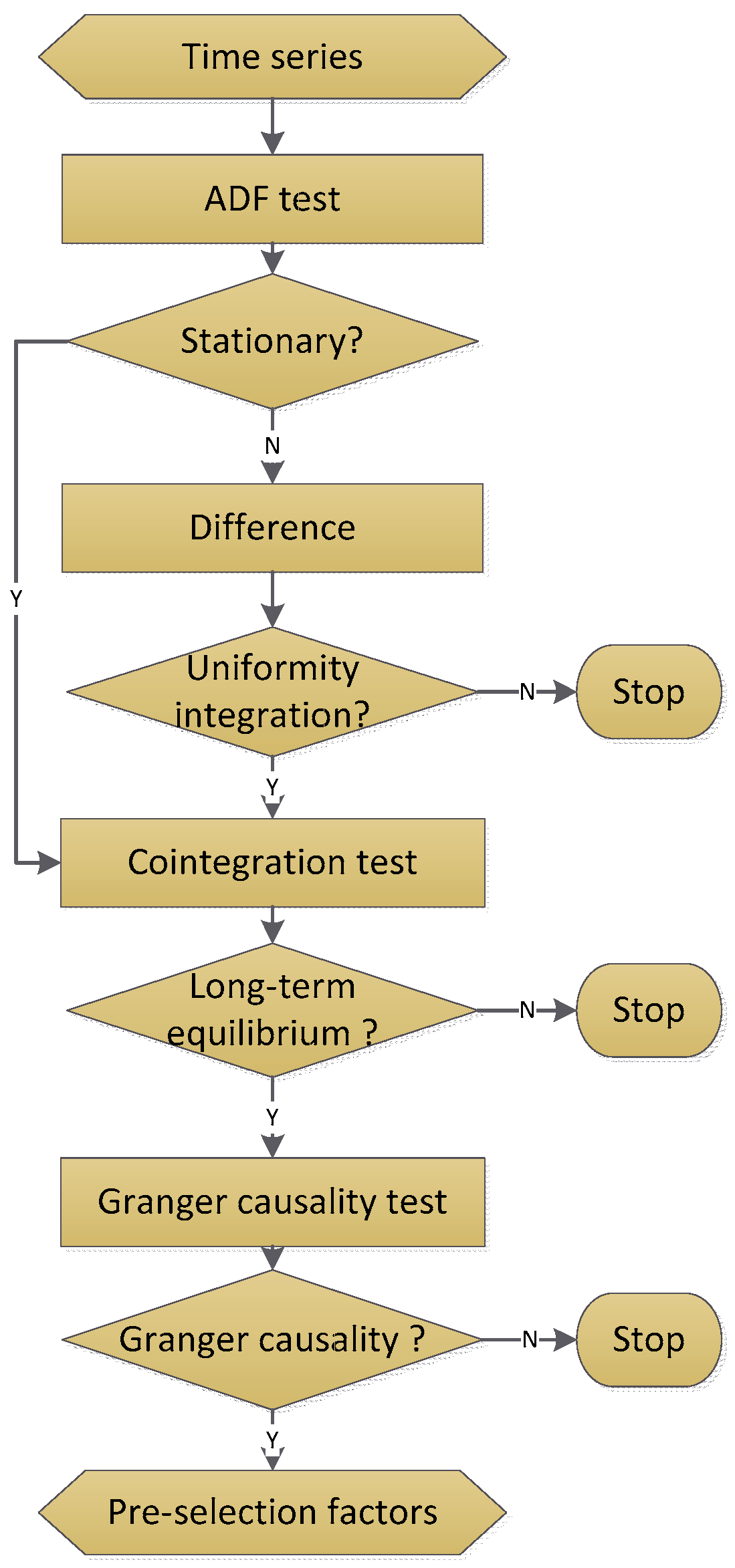
At present, there are few literatures on carbon price prediction considering both internal factors (carbon price historical data) and external factors (the influencing indicators of the carbon price, such as energy price, economic index, and so on). Most of the literature only predicts carbon prices based on historical data or only studies the relationship between carbon prices and their influencing factors. Therefore, historical data determined by partial autocorrelation function (PACF) and influencing indicators selected by the augmented Dickey–Fuller (ADF) test, cointegration test, and granger causality test are both used to predict carbon prices at the same time in this paper.

In addition, the data selected in the empirical research part of most of the literature come from one market, such as the EU emissions trading scheme (EU ETS) or China ETS. To verify the versatility of the model built in this paper, the empirical part of this paper will select both EU ETS and China ETS to study. The main contributions of this article are as follows:

• The carbon price forecast not only considers internal factors (historical carbon price data) but also considers external factors, including energy prices and economic factors, which makes the forecast more comprehensive and accurate.
• The MFO-optimized ELM, called MFO-ELM, was selected as the predictive model. The MFO-ELM model has the ability to maximize the global search ability of the MFO and the learning speed of the ELM and solve the intrinsic instability of the ELM by optimizing its parameters.
• Using MRSVD to decompose the historical carbon price sequences and selecting partial autocorrelation function (PACF), we can determine the lag data as internal factors, which are a part of the MFO-ELM input.
• Combining ADF testing, cointegration testing, Granger causality testing, we can select external factors; this is another part of the MFO-ELM input.
• The carbon price dates of the EU ETS and the China ETS were both collected and predicted with the intention of testing the universality of the proposed model.

This paper’s framework is as below: Section 2 shows methods and models employed in this paper, which includes MRSVD, MFO, and ELM. The entire framework of the proposed model (MRSVD-MFO-ELM) is then detailed in Section 3. Section 4 presents empirical studies, including data collection, external and internal input selection, parameter settings, prediction results, and error analysis for EU ETS and China ETS. Conclusions in view of the results are shown in Section 5.

2. Methodology

This section highlights a brief introduction to the methods used in this article. Therefore, a brief review of the theory involved, namely the ADF test, cointegration test, and Granger causality test, MRSVD, PACF, MFO, and ELM, is shown below, respectively.

2.1. ADF Test

If a time series meets the following conditions: (1) Mean $E\left(X_t\right)=\mu$ is a constant independent of time t. (2) Variance $Var\left(X_t\right)={\sigma }^2$ is a constant independent of time t. (3) Covariance $Cov\left(X_{t,}{X}_{t+k}\right)={\gamma }_k$ is a constant only related to time interval k, independent of time t, then, the time series is stationary.

The ADF test is a way to determine whether a sequence is stable. For the regression $X_t=\rho X_{t-1}+{\mu }_t$. If $\rho$ = 1 is found, the random variable $X_t$ has a unit root, then the sequence is not stable; otherwise, there is no unit root, and the sequence is stable.

2.2. Cointegration Test

If a non-stationary time series becomes smooth after 1-differential $\Delta X_t=X_t-X_{t-1}$, the original sequence is called integrated of 1, which is denoted as I(1). Generally, if one non-stationary time series becomes smooth after d-differential, the original sequence is called integrated of d, which is denoted as I(d).

For two non-stationary time series $\left\{X_t\right\}$ and $\left\{Y_t\right\}$, if $\left\{X_t\right\}$ and $\left\{Y_t\right\}$ are both $I\left(d\right)$ sequences, and there is a linear combination $X_t+b{Y}_t$ making $\left\{X_t+b{Y}_t\right\}$ a stationary sequence, then there is a cointegration relationship between $\left\{X_t\right\}$ and $\left\{Y_t\right\}$.

2.3. Granger Causality Test

If variable X does not help predict another variable Y, then X is not the cause of Y. Instead, if X is the cause of Y, two conditions must be met: (1) X should help predict Y. That is to say, adding the past value of X as an independent variable should significantly increase the explanatory power of the regression; (2) Y should not help predict X, because if X helps predict Y, Y also helps in predicting X, there is likely to be one or several other variables, which are both the cause of the X and Y. This causal relationship, defined from the perspective of prediction, is generally referred to as Granger causality.

Estimate two regression equations:

Unconstrained regression model (u)

$$Y_t={\alpha }_0+{\displaystyle \sum }_{i=1}^p{\alpha }_i{Y}_{t-i}+{\displaystyle \sum }_{i=1}^q{\beta }_i{X}_{t-i}+{\epsilon }_t.$$

(1)

Constrained regression model (r)

$$Y_t={\alpha }_0+{\displaystyle \sum }_{i=1}^p{\alpha }_i{Y}_{t-i}+{\epsilon }_t$$

(2)

${\alpha }_0$ represents a constant term, $p\mathrm{and}q$ are the maximum lag periods of Y and X, respectively. ${\epsilon }_t$ is white noise.

Then use the residual squared sum ($RSS$) of the two regression models to construct the F statistic.

$$F=\frac{\left(RS{S}_r-RS{S}_u\right)/q}{RS{S}_u/\left(n-p-q-1\right)}~F\left(q,n-p-q-1\right).$$

(3)

where n is the sample size:

Test null hypothesis $H_0$: X is not the Granger cause of Y ($H_0$: ${\beta }_1={\beta }_2=\cdots ={\beta }_q=0$)

If $F>F_{\alpha }\left(q,n-p-q-1\right)$, then ${\beta }_1,{\beta }_2,\cdots ,{\beta }_q$ is not zero significantly. The null hypothesis $H_0$ should be rejected; otherwise, $H_0$ cannot be rejected.

Akaike information criterion (AIC) is used for judging lag orders in the Granger causality test. AIC is defined as

$$AIC=2k-2ln\left(L\right)$$

(4)

where $k$ is the number of model parameters, representing the complexity of the model, and $L$ is the likelihood function, representing the fitting degree of the model. The goal is to select the model with the minimum AIC. AIC should not only improve the model fitting degree but also introduce a penalty term to make the model parameters as little as possible, which helps to reduce the possibility of overfitting.

2.4. MRSVD

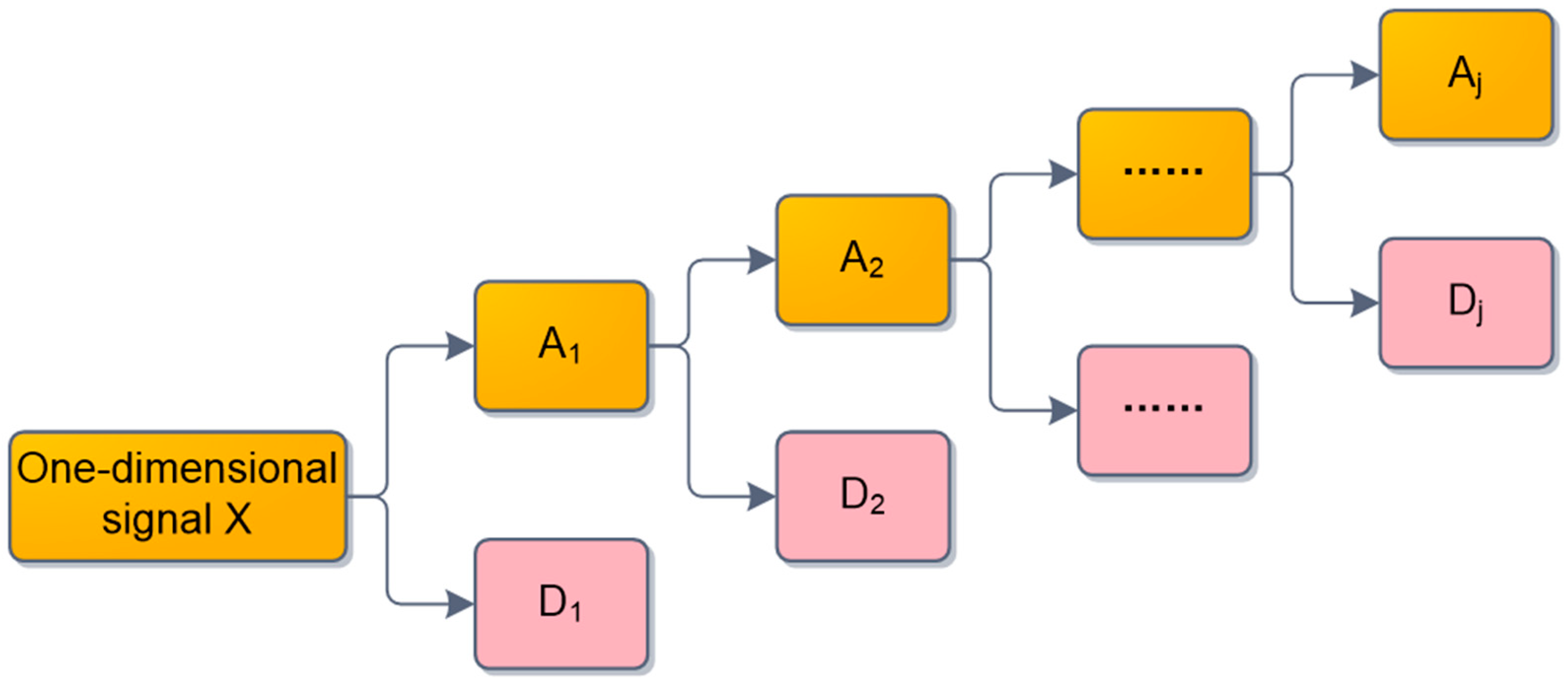
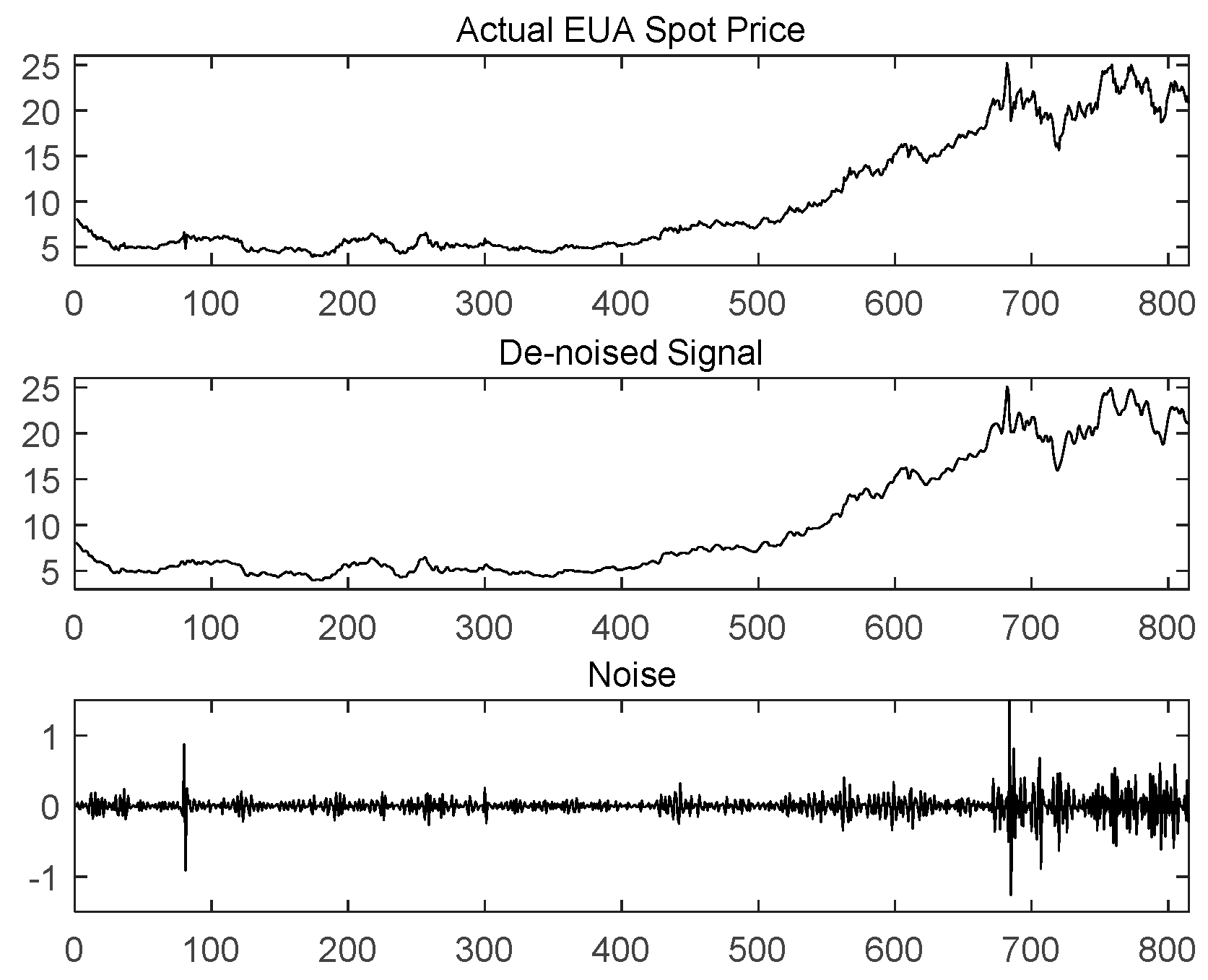
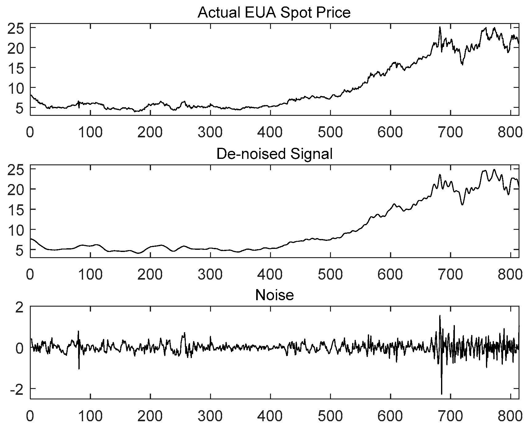
Based on SVD, MRSVD draws on the idea of wavelet multi-resolution [32] and uses the two-way recursive idea to construct the Hankel matrix to analyze the signal [33], which realizes a decomposition of complex signals into sub-spaces of different levels. The core idea of MRSVD is to first decompose the original signal X into the detail signal (D1) and with less correlation with the original signal and the approximation signal (A1) with more correlation with the original signal, and then decompose A1 by SVD recursively. Finally, the original signal is decomposed into a series of detail signals and approximation signals with different resolutions [34]. Specific steps are as follows:

First, construct a Hankel matrix for one-dimensional signal $X=\left(x_1,x_2,x_3\cdots x_N\right)$.

$$H=\left(\begin{array}{cccc}{x}_1& x_2& \cdots & x_{N-1}\\ x_2& x_3& \cdots & x_N\end{array}\right)$$

(5)

Then perform SVD on the matrix H to obtain:

$$H=US{V}^T=\left[u_1{u}_2\right]\left[\begin{array}{l}{\delta }_{1}00\cdots 0\\ 0{\delta }_{1}0\cdots 0\end{array}\right]\left[\begin{array}{c}{v_1}^T\\ {v_2}^T\\ ⋮\\ 0\end{array}\right]$$

(6)

Among them, ${\delta }_1$ and ${\delta }_2$ are singular values obtained by decomposition, ${\delta }_1\ge {\delta }_2$, $u_1,u_2,v_1,v_2$ are, respectively, column vectors obtained after SVD decomposition; $H={\delta }_1{u}_1{v_1}^T+{\delta }_2{u}_2{v_2}^T$, $A_1={\delta }_1{u}_1{v_1}^T$, corresponds to the large singular value, reflecting the approximation component of H; $D_1={\delta }_2{u}_2{v_2}^T$, corresponds to the small singular, reflecting the detailed component of H.; Continue to perform SVD on ${\mathrm{A}}_1$, and the decomposition process is shown in Figure 1 [35].

MRSVD for one-dimensional discrete signals shows that there is a certain difference between MRSVD and WT. The number of decomposition layers of WT is limited, and MRSVD is not limited by the number of decomposition layers. Multi-level multi-resolution of the original signals can be performed by MRSVD. To prevent the energy loss of the signal, the number of components in the signal decomposition process is two. According to the above steps, the original signal can reflect the detail signal and the approximate signal through multiple levels, and finally, the inverse of the extracted signal is performed. The structure can realize the noise reduction and feature extraction of the original signal.

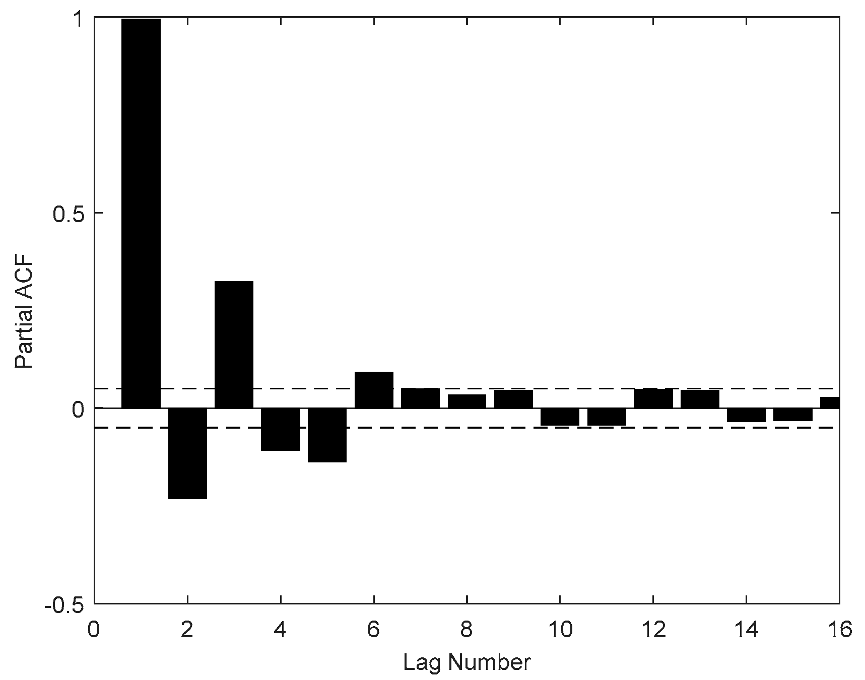
2.5. PACF

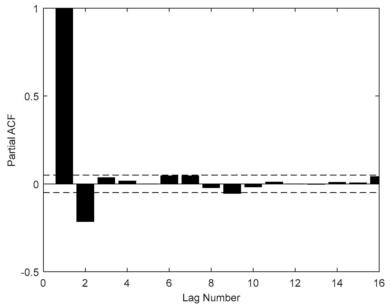
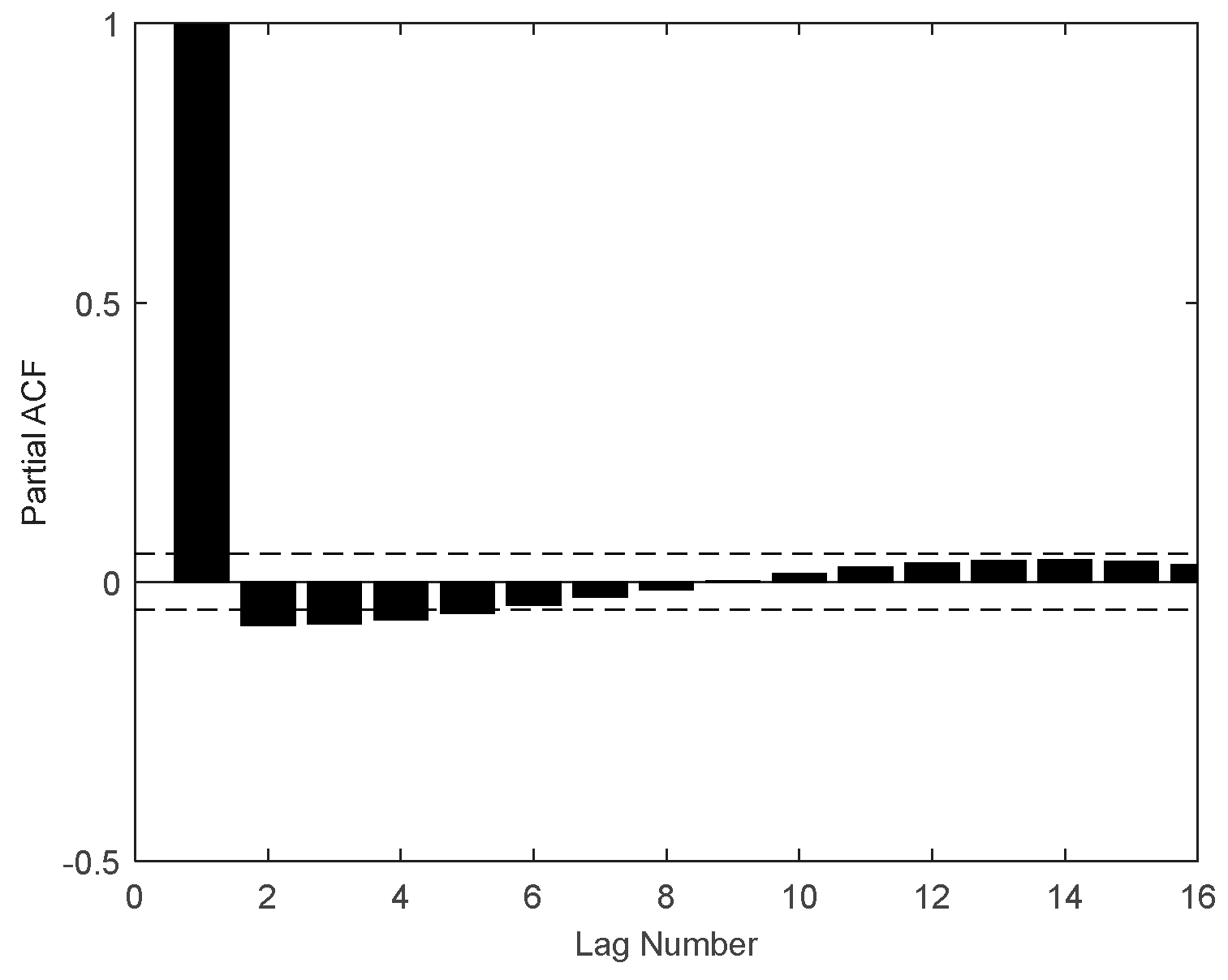
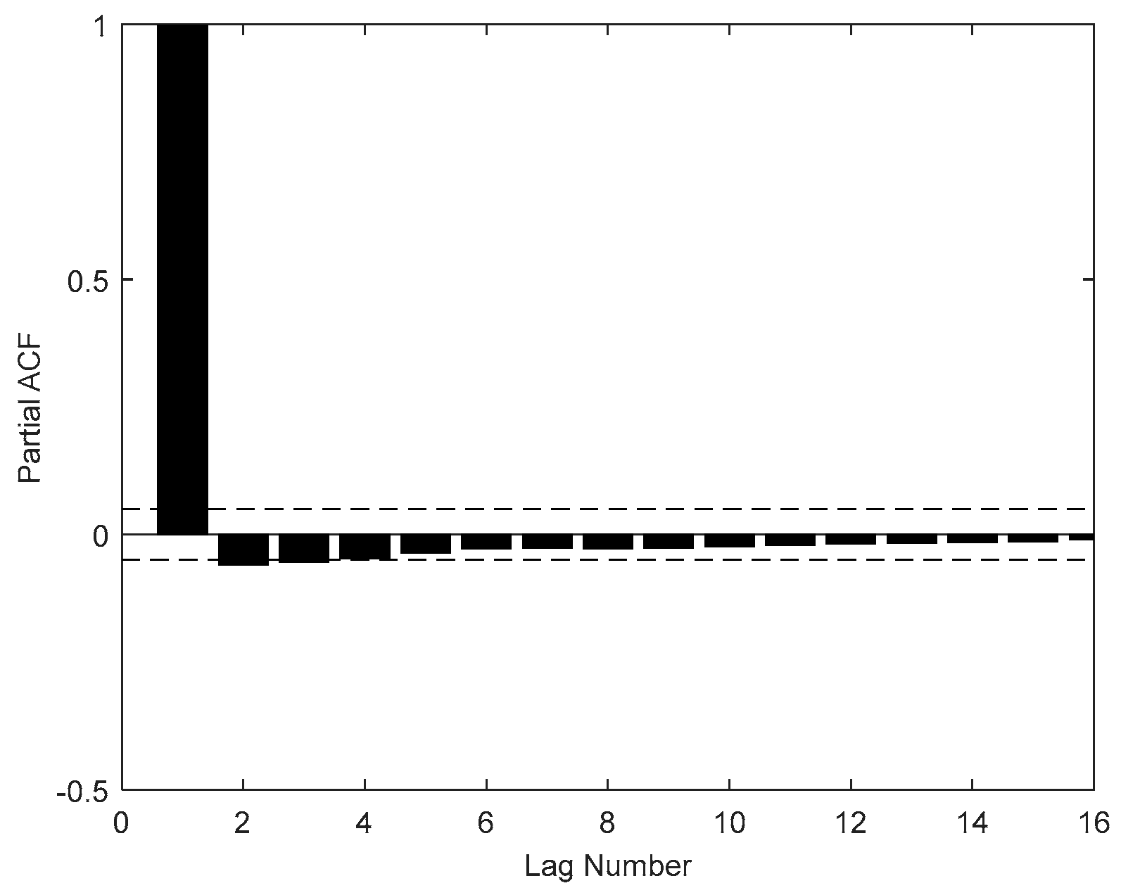
The partial autocorrelation function (PACF) is a commonly used method that describes the structural characteristics of a stochastic process, which gives the partial correlation of a time series with its own lagged values, controlling for the values of the time series at all shorter lags.

Given a time series $x_t$, the partial autocorrelation of lag $\mathrm{k}$, is the autocorrelation between $x_t$ and $x_{t-k}$ that is not accounted for by lags 1 to k − 1. Described in mathematical language is as follows:

Suppose that the k-order autoregressive model can be expressed as

$$x_t={\Phi }_{k1}{x}_{t-1}+{\Phi }_{k2}{x}_{t-2}+\cdots +{\Phi }_{kk}{x}_{t-k}+u_t$$

(7)

where ${\Phi }_{kj}$ represents the $j$-th regression coefficient in the $k$-th order autoregressive expression, and ${\Phi }_{kk}$ is the last coefficient.

2.6. Moth–Flame Optimization Algorithm

The MFO algorithm is a cluster intelligent optimization algorithm based on the behavior of moths flying close to the flame in the dark night. The algorithm uses the moth population M and the flame population F to represent the solution to be optimized. The role of the moth is to constantly update the movement and finally find the optimal position, while the role of the flame is to preserve the optimal position found by the current moth. The moths are in one-to-one correspondence with the flames, and each moth searches for the surrounding flame according to the spiral function. If a better position is found, the current optimal position saved in the flame is replaced. When the iterative termination condition is satisfied, the optimal moth position saved in the output flame is the optimal solution for the optimization problem [36].

In the MFO algorithm, the moth is assumed to be a candidate solution. The variable of the problem is the position of the moth in space. The position matrix of the moth can be expressed as M, and the vector storing its fitness value is $OM$.

$$\begin{array}{c}M=\left[\begin{array}{cccc}{M}_{11}& M_{12}& \cdots & M_{1d}\\ M_{21}& M_{22}& \cdots & M_{2d}\\ ⋮& ⋮& \cdots & ⋮\\ M_{n1}& M_{n2}& \cdots & M_{nd}\end{array}\right]\\ OM=\left[\begin{array}{c}O{M}_1\\ O{M}_2\\ ⋮\\ O{M}_n\end{array}\right],\end{array}$$

(8)

where n is the number of moths; d is the number of variables.

Another important component of the MFO algorithm is the flame. Its position matrix can be expressed as F, and the matrices M and F have the same dimension. The vector storing the flame adaptation value is $OF$:

$$\begin{gathered} F=\left[\begin{array}{cccc}{F}_{11}& F_{12}& \cdots & F_{1d}\\ F_{21}& F_{22}& \cdots & F_{2d}\\ ⋮& ⋮& \cdots & ⋮\\ F_{n1}& F_{n2}& \cdots & F_{nd}\end{array}\right] \\ OF=\left[\begin{array}{c}O{F}_1\\ O{F}_2\\ ⋮\\ O{F}_n\end{array}\right] \end{gathered}$$

(9)

The $MFO$ algorithm is a three-dimensional method for solving the global optimal solution of nonlinear programming problems, which can be defined as

$$MFO=\left(I,P,T\right)$$

(10)

where I is a function that can generate random moths and corresponding fitness values. The mathematical model of the function I can be expressed as

$$I:\varnothing \to \left\{M,OM\right\}$$

(11)

The function $P$ is the main function, which can freely move the position of the moth in the search space. The function $P$ records the final position of the moth through the update of the matrix $M$.

$$P:M\to M$$

(12)

The function T is the termination function. If the function T satisfies the termination condition, ‘true’ will be returned, and the procedure will be stopped; otherwise, ‘false’ will be returned, and the function P will continue to search.

$$T:M\to \left\{true,false\right\}$$

(13)

The general framework for describing MFO algorithms using I, P, and T is defined as follows:

M = I();

while T(M) is equal to false

M = P(M);

End

After function I is initialized, function P iterates until function T returns true. To accurately simulate the behavior of the moth, Equation (14) is used to update the position of each moth relative to the flame:

$$M_i=S\left(M_i,F_j\right)=D_i·e^{bt}·cos\left(2\pi t\right)+F_j$$

(14)

Here $M_i$ denotes the i-th moth, $F_j$ denotes the j-th flame, and S denotes a logarithmic spiral function. $D_i$ represents the distance between the i-th moth and the j-th flame, b is a constant defining the shape of the logarithmic spiral, and t is a random number between [−1,1]. $D_i$ is calculated by the Equation (15):

$$D_i=\left|F_j-M_i\right|$$

(15)

Additionally, another problem here is that location updates of moths relative to n different locations in the search space may reduce the exploitation of the best promising solutions. With this in mind, an adaptive mechanism capable of adaptively reducing the number of flames in the iterative process is proposed to ensure fast convergence speed. Use the following equation in this regard:

$$flameno=round\left(N-l\cdot \frac{N-1}{T}\right)$$

(16)

where $l$ is the current number of iterations, N is the maximum number of flames, and T is the maximum number of iterations [37].

2.7. Extreme Learning Machine

ELM is a single hidden layer feedforward neural network (Single-hidden layer feedforward neural network). Its main feature is that the connection weights between the input layer and hidden layer w (the hidden layer neuron threshold) are randomly initialized, the network converting the training problem of the network into a solution to directly find a linear system. Unlike the traditional gradient learning algorithm, which requires multiple iterations to adjust the weight parameters, ELM has the advantages of short training time and small calculation [38].

The ELM consists of an input layer x₁ … x_n, a hidden layer, and an output layer y₁ … y_n, where the input layer neuron number is n, the hidden layer neuron number is L, and the output layer neuron number is m.

The connection weights between the input layer and the hidden layer are $\omega ={\left[{\omega }_{ij}\right]}_{n\times L},i=1\cdots n,j=1\cdots L$, and the connection weights between the hidden layer and the output layer are $\beta ={\left[{\beta }_{jk}\right]}_{L\times m},j=1\cdots L,k=1\cdots m$.

Make the training set input matrix with Q samples to be $X={\left[x_{ir}\right]}_{n\times Q},i=1\cdots n,r=1\cdots Q,$ output matrix to be $Y={\left[y_{kr}\right]}_{m\times Q,}k=1\cdots m,r=1\cdots Q,$ the hidden layer neuron threshold is $b={\left[b_1,b_2\cdots b_L\right]}^T$ the hidden layer activation function is $g\left(x\right).$ The expected output of the network is $T=\left[t_1,t_2\cdots t_m\right]$ [39]. Therefore, ELM can be illustrated as

$$T^{\prime }=\left[\begin{array}{c}{t}_1\\ t_2\\ ⋮\\ t_m\end{array}\right]=\left[\begin{array}{c}{\displaystyle \sum _{j=1}^L{\beta }_{j1}g\left(w_j·x_i+b_j\right)}\\ {\displaystyle \sum _{j=1}^L{\beta }_{j2}g\left(w_j·x_i+b_j\right)}\\ ⋮\\ {\displaystyle \sum _{j=1}^L{\beta }_{jm}g\left(w_j·x_i+b_j\right)}\end{array}\right]i=1\cdots n$$

(17)

However, random parameter settings not only improve the learning speed of ELM but also increase the risk of getting expected results simultaneously. Therefore, this paper uses MFO to search for the best optimal parameters, including the input weight and the bias in the hidden layer, to improve the training process and avoid over-fitting.

3. The Whole Framework of the Proposed Model

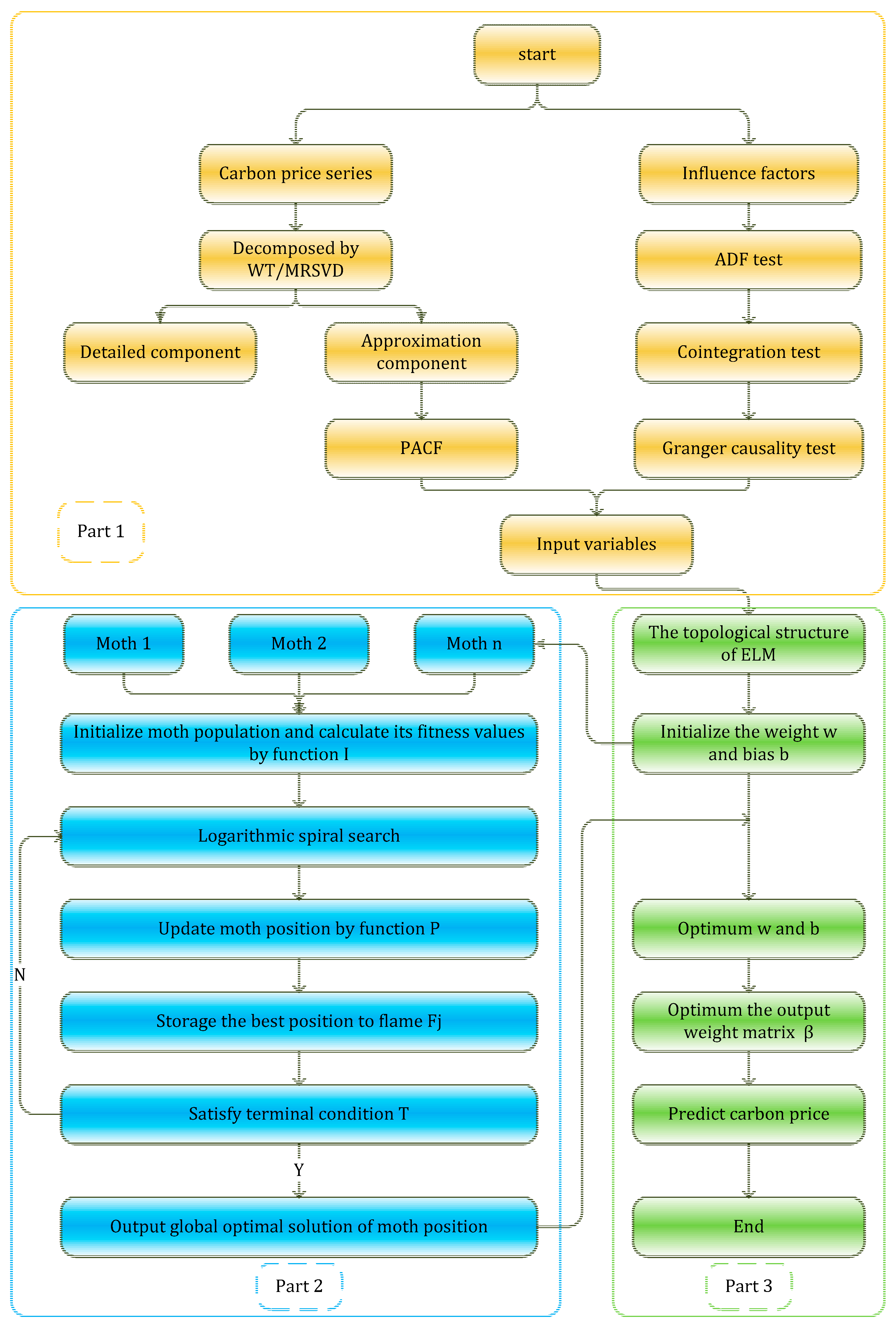
Figure 2 introduces the overall idea and frame of the article. There are three parts with different colors yellow, green, and blue.

Part 1 describes the input indicator selection procedure. The input variables used in ELM include two parts, external factors analyzed by the ADF test, cointegration test and Granger causality test, internal factors, and internal factors of the carbon price decomposed by WT and MRSVD, respectively, whose lags are determined by the PACF.

Part 2 mainly introduces the process of MFO. The purpose of this part is optimizing the parameter weight w and bias b of the ELM.

Part 3 is the ELM’s training procedure, whose set data can be obtained in Part 1, and Part 2 optimizes the parameters of the ELM. Thus, the carbon price prediction result can be obtained by the optimized ELM model.

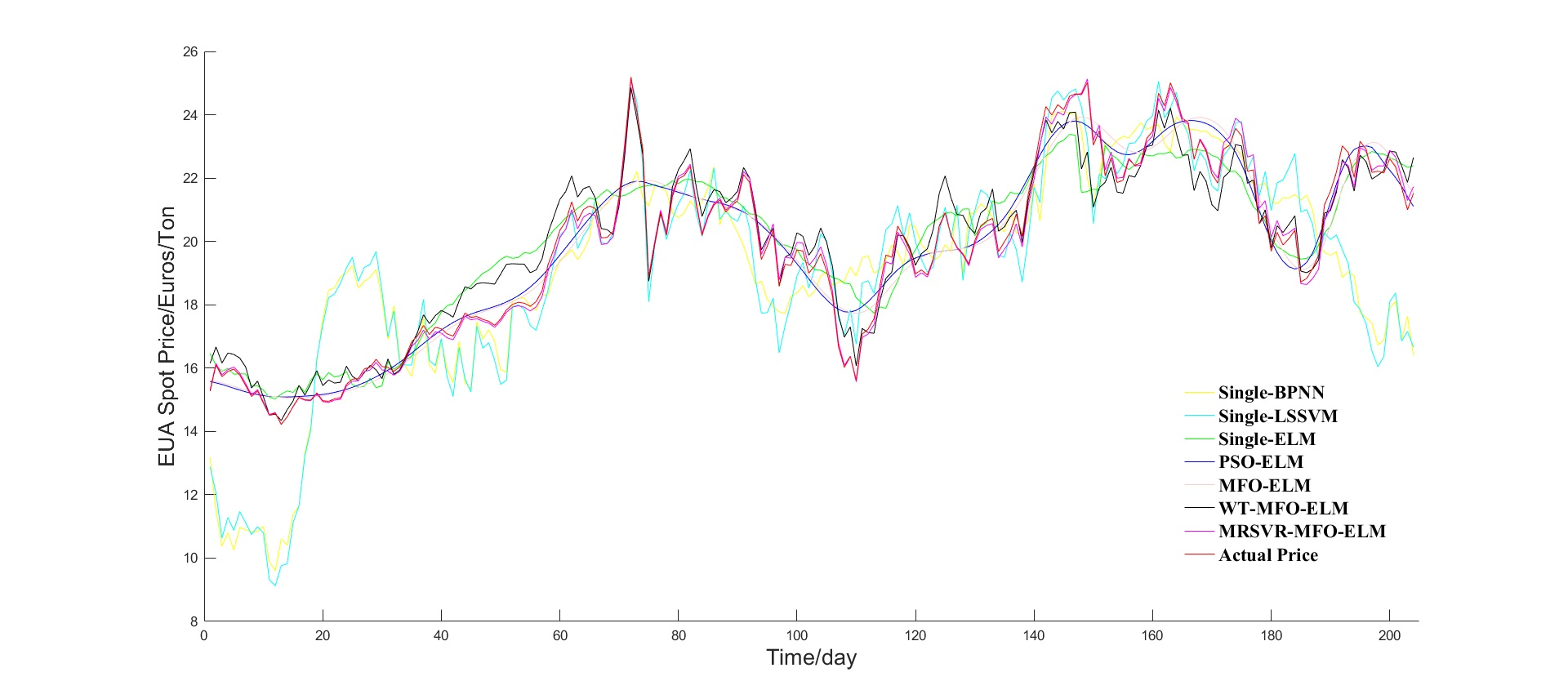
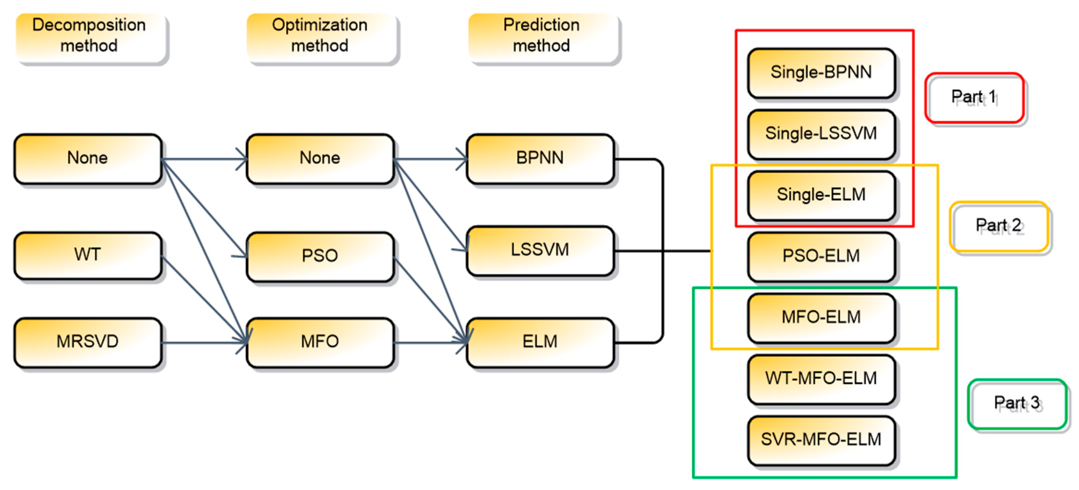
To verify the superiority of the proposed model, a comparison framework is shown in Figure 3, which includes three sections.

In section 1, single BPNN, single LSSVM, and single-ELM were congregated to present the predictive performance of three neural network models and verify the advantages of single ELM.

In section 2, single-ELM, PSO-ELM, and MFO-ELM were collected to demonstrate the necessity of optimizing the parameter of ELM, and verify the advantages of MFO compared with PSO.

In section 3, MFO-ELM, WT-MFO-ELM, MRSVD-MFO-ELM were used to demonstrate the effectiveness of the carbon price decomposition process and the advantage of MRSVD.

4. Empirical Analysis

4.1. Case Studies of the EU Carbon Price

4.1.1. Data Collection

The EU ETS is the world’s largest carbon trading system at present, accounting for about 90% of the global carbon trading scale. The EU ETS includes European emission allowances (EUA) spot market and future market, hence, EUA spot price and three main EUA future price with maturity in December 2019 (DEC19), December 2020 (DEC20), December 2021 (DEC21) were collected, EUA spot price, DEC19, DEC20 data are all from 4 January 2016 to 21 March 2019, and DEC20 is from 26 September 2016 to 21 March 2019. Figure 4 depicts the daily carbon price curve for the EUA spot price, DEC19, DEC20, and DEC21 in Euros per ton, which comes from European Energy Exchange (EEX) [40]. The abscissa of Figure 4 represents the sample number, and its ordinate represents EUA spot price, DEC19 price, DEC20 price, and DEC21 price respectively. As can be seen from Figure 4, the four types of carbon prices have striking similarities. Therefore, this paper only selects the EUA spot price as an experimental sample.

In this paper, five indicators, including EUA spot trading volume, CSX coal future price (coal price), crude oil future price (oil price), natural gas future price (gas price), and Euro Stoxx 50 were used as the influence pre-selection factors of the EUA spot price. EUA spot trading volume data were from EEX [34], CSX coal future price data were from ICE [41], crude oil future price and natural gas future price data were from EIA [42], Euro Stoxx 50 data were from Investing [43]. The data collection range of these indicators was all 4 January 2016 to 21 March 2019, which is illustrated in Figure 5. The abscissa of Figure 5 represents the sample number, and its ordinate represents EUA spot price, EUA spot trading volume, CSX coal price, crude oil future price, natural gas future price and Euro Stoxx 50 respectively.

4.1.2. Input Selection

1. External Factor Selection

Combined with the ADF test, cointegration test, and Granger causality test under the environment of Eviews 7.0, the relationship between variables is accurately judged, and the input factors of MFO-ELM are selected. The flow is shown in Figure 6.

(a) The ADF test

A prerequisite for Granger causality testing is that the time series must be stationary. Otherwise, pseudo-regression problems may occur. Therefore, the unit root test should be performed before the Granger causality test. In this paper, the ADF test is used to perform unit root test on the stationarity of each index sequence, as shown in

Table 1. The augmented Dickey–Fuller (ADF) test results for European emission allowances (EUA) spot price and its external factors.

Test Variable.	t-Statistic	Prob. *	Test Variable	t-Statistic	Prob. *
EUA Spot Price	−1.75758	0.7242	d(EUA Spot Price)	−6.346582	0
Coal Price	−0.863377	0.958	d(Coal Price)	−26.38188	0
Oil Price	−2.066305	0.5633	d(Oil Price)	−28.82263	0
Gas Price	−1.845876	0.3582	d(Gas Price)	−23.00113	0
Euro Stoxx 50	−1.8626	0.3502	d(Euro Stoxx 50)	−27.764	0
EUA Spot Trade Volume	−14.60444	0	-	-	-

* MacKinnon (1996) one-sided p-values.

.

As seen in Table 1, the EUA spot price, coal price, gas price, oil price, and Euro Stoxx 50 are not stationary sequences. However, the sequences are all stable when the first difference is made. But the EUA spot trading volume is a stationary sequence. That is, these series all submit to the identical order except the EUA spot trading volume.

(b) Cointegration test

When all the test series submit to the identical order I(d), the vector autoregression model (VAR) model can be constructed to perform the cointegration test to decide the existence of cointegration relationship and long-term equilibrium relationship between the variables. That is, the premise of the cointegration test is that all the test series submit to the identical order. As shown in Table 1, the EUA spot price, CSX coal future price, crude oil future price, natural gas future price, and Euro Stoxx 50 are all I(1) and can be used for cointegration test, while the EUA spot trading volume is I(0), that is to say, the long-term balanced relationship between EUA spot trading volume and EUA spot price does not exist, then it is abandoned. This article considers the Johansen test, an effective tool to measure the long-term relationships between variables, and to operate cointegration analysis between the variables. Cointegration test results can be seen in

Table 2. Cointegration test results for EUA spot price and its external factors.

Test Variables	Hypothesized No. of CE(s)	Eigenvalue	Trace Statistic	0.05 Critical Value	Prob. **
EUA Spot Price and Coal Price	None *	0.120923	112.8137	15.49471	0.0001
	At most 1 *	0.026159	19.24447	3.841466	0
EUA Spot Price and Oil Price	None *	0.146913	117.0423	15.49471	0.0001
	At most 1 *	0.027394	17.41576	3.841466	0
EUA Spot Price and Gas Price	None *	0.182831	142.8526	15.49471	0.0001
	At most 1 *	0.028096	17.66877	3.841466	0
EUA Spot Price and Euro Stoxx 50	None *	0.220548	201.6133	15.49471	0.0001
	At most 1 *	0.026289	19.47446	3.841466	0

*: denotes rejection of the hypothesis at the 0.05 level. **: MacKinnon–Haug–Michelis (1999) p-values.

.

Table 2 demonstrates that there is a cointegration relationship between the EUA spot price and coal price, oil price, gasoline price, Euro Stoxx 50, which is the foundation of the Granger causality test.

(c) Granger causality test

Results from the cointegration test verify that there is a long-term relationship between pre-selected external factors and EUA spot prices, but their causality has not been introduced. Therefore, it is highly desirable to perform the Granger causality test to analyze the Granger causality between two variables. The Akaike information criterion was used to choose the lag, and the Granger causality test results are presented in

Table 3. Granger causality test results for EUA spot price and its external factors.

Test Variables	F-Statistic	Prob.	Lag	Conclusion
Coal Price→EUA Spot Price	4.06991	0.0174	2	Exist a Granger causality
EUA Spot Price→Coal Price	1.08564	0.3382	2	Not exist a Granger causality
Oil Price→EUA Spot Price	13.0678	0.0003	1	Exist a Granger causality
EUA Spot Price→Oil Price	0.23313	0.6294	1	Not exist a Granger causality
Gas Price→EUA Spot Price	31.104	3.0 × 10−8	1	Exist a Granger causality
EUA Spot Price→Gas Price	0.08135	0.7756	1	Not exist a Granger causality
Euro Stoxx 50→EUA Spot Price	20.8186	6.0 × 10−6	1	Exist a Granger causality
EUA Spot Price→Euro Stoxx 50	0.02983	0.8629	1	Not exist a Granger causality

.

As can be seen from Table 3, the EUA spot price was not the Granger cause of the price of coal, oil, gas, and Euro Stoxx 50, but they were the Granger cause of EUA spot price under certain lag phases. This paper selected coal price 1 and 2 years ahead (Lag 2), oil price 1 year ahead (Lag 1), gas price 1 year ahead (Lag 1) and Euro Stoxx 50 1 year ahead (Lag 1) as variables for MFO-ELM input when predicting the EUA spot price.

2. Internal Factor Selection

(a) Carbon price decomposition

With the intention of reducing noise influence, WT and MRSVD were utilized, respectively, to decompose the time series and remove the stochastic volatility. The abscissa of Figure 7 and Figure 8 are both represent the sample number, and their ordinate represent actual EUA spot price, de-noised signal and noise respectively. It can be seen in Figure 7 and Figure 8 that the EUA spot price sequences are divided into an approximate component A1 (de-noised signal) and a detail component D1 (noise signal). The former will show carbon price’s major wave motion, while the later contains peak and random volatility. Compared to the original carbon price, A1 offers a smooth form, while D1 presents high-frequency sections. Consequently, A1 was taken as the carbon price with the intention of increasing efficiency, and it owns a smaller phase shift and less waveform distortion when decomposed by MRSVD.

(b) Lags determination by PACF

To test the correlation between historical prices quantities and the prices targeted, this paper introduced PACF to choose the models’ input variables. Namely, PACF was utilized to discover hysteresis, which is important when internal correlation has been eliminated. Figure 9, as well as Figure 10, illustrates the results of PACF for approximate components of the EUA spot price after WT and MRSVD, respectively.

Set xi as the output variable. If the PACF at lag k exceeds the 95% confidence interval, choose xi–k as one of the input variables.

Table 4. The results of external and internal input factors selection for EUA spot price forecasting.

External Input Factors	Internal Input Factors by WT	Internal Input Factors by MRSVD
Coal Price (t-1)	EUA Spot Price (t-1)	EUA Spot Price (t-1)
Coal Price (t-2)	EUA Spot Price (t-2)	EUA Spot Price (t-2)
Oil Price (t-1)		EUA Spot Price (t-3)
Gas Price (t-1)		EUA Spot Price (t-4)
Euro Stoxx 50 (t-1)		EUA Spot Price (t-5)

presents the external and internal input variables for the EUA spot price after WT and MRSVD for MFO-ELM.

4.1.3. Parameters Setting and Forecasting Evaluation Criteria

For those parameter settings likely to influence the forecast precision, it is indispensable to appoint the parameters of the proposed model and its comparison models. The specifications are presented in

Table 5. Parameters of the proposed model and its comparison models.

Model	Parameters
BPNN	Hidden layer node = 7; Learning rate = 0.0005
LSSVM	γ = 50; δ2 = 2
ELM	Hidden layer node = 10, g(x) = ‘sig’
PSO	Sizepop = 20; Maxgen = 500; The search band = [−5,5]; c1 = c2 = 1.49445; w = 0.729
MFO	Sizepop = 20; Maxgen = 500; The search band = [−5,5]

.

γ denotes the regularization parameter, δ² is the core parameter, γ denotes the regularization parameter, g(x) denotes the hidden layer activation function, Sizepop denotes the initial population size, Maxgen denotes the maximum number of iterations, c1 and c2 are acceleration factors, and w is inertia weight. Each parameter in Table 5 is consistently revised through simulation to get ideal results. To effectively measure prediction capability, this paper puts forward common error criteria to examine the precision of models related, which include mean absolute error ($MAE$), mean absolute error $(MAPE$), root mean square error ($RMSE$) and $R^2$ determination coefficient. The equations are expressed as follows:

$$MAE=\frac{1}{n}\left|y_i-{y_i}^{*}\right|,$$

(18)

$$MAPE=\frac{1}{n}{{\displaystyle \sum }}_{i=1}^n\left|\frac{y_i-{y_i}^{*}}{y_i}\right|\times 100\%,$$

(19)

$$RMSE=\sqrt{\frac{1}{n}{{\displaystyle \sum }}_{i=1}^n{\left|\frac{y_i-{y_i}^{*}}{y_i}\right|}^2},$$

(20)

$$R^2=\frac{{\left(n{{\displaystyle \sum }}_{i=1}^n{y}_i\times {y_i}^{*}-{{\displaystyle \sum }}_{i=1}^n{y}_i{{\displaystyle \sum }}_{i=1}^n{y_i}^{*}\right)}^2}{\left(n{{\displaystyle \sum }}_{i=1}^n{{y_i}^{*}}^2-{\left({{\displaystyle \sum }}_{i=1}^n{y_i}^{*}\right)}^2\right)\left(n{{\displaystyle \sum }}_{i=1}^n{y_i}^2-{\left({{\displaystyle \sum }}_{i=1}^n{y}_i\right)}^2\right)},$$

(21)

where n represents the number of training samples, and $y_i$ and ${y_i}^{*}$ are actual and predicted values.

4.1.4. EUA Spot Price Forecasting

The specimen contains two subsets: training set and testing set. The 610 data from 1 April 2016 to 31 May 2018 are used as the training set, and the 204 data from1 June 2018 to 20 March 2019 are used as the testing set. The training set was utilized to build the forecasting model, while the testing set was utilized to examine the model’s robustness. And then, the proposed MFO-ELM model for EUA spot price forecasting was implemented in MATLAB 2016a on a Windows 7 system.

Figure 11 shows the convergence curve of the MFO. It is obvious that as the times of iterations increased, the fitness curve sloped downward and tended to stabilize at the 100th generation iteration, it meant that MFO operates ideally when finding the best parameters.

As shown in Figure 12, it is clear that the MRSVR-MFO-ELM model owns a better fit curve than the other comparison models. The results of WT-MFO-ELM, MFO-ELM, and PSO-ELM performed slightly worse in terms of suitability, while single ELM, single LSSVM, single BP showed the worst performance, and their points deviated from the true value.

Figure 13 plots a histogram that shows the comparison of MAE, MAPE, RMSE and R² clearly and visually. We can draw the following conclusions from Figure 13:

(a) MRSVD-MFO-ELM provides the best prediction of the EUA spot price based on the evaluation indicators in MAE, MAPE, RMSE and $R^2$. The MAE, MAPE and RMSE’s values of MRSVD-MFO-ELM were 0.151580, 0.007464, 0.009248, respectively, which were much smaller than MAE, MAPE, RMSE’s values of single BPNN 1.642773, 0.088583, 0.122379. The $R^2$ value of MRSVD-MFO-ELM was 0.995465, which was much larger than the R² value of single BPNN 0.599798, showing the good performance of MRSVD-MFO-ELM in the EUA spot price forecast.

(b) Compare single ELM with single BP and single LSSVM to verify the correctness of the prediction algorithm selection. The best performance of single ELM in MAE was 0.828777, MAPE was 0.041909, RMSE was 0.053768, $R^2$ was 0.863472. It was more ideal than single BP and single LSSVM, indicating that ELM is a kind of model more appropriate for forecasting EUA spot price.

In addition, it can be seen that there were significant gaps between the first two models and the last five ones. The first two models were based on BPNN and LSSVM, respectively, while the last five models were all ELM-based models, showing that the selection of forecasting model is of vital importance in the EUA spot price forecast.

(c) Compare PSO-ELM, MFO-ELM, and single ELM to verify the importance of the optimization algorithm. The models with optimization algorithm (PSO-ELM, MFO-ELM) had smaller MAE, MAPE, RMSE and larger $R^2$ than models without optimization algorithm (single ELM). Therefore, the conclusion could be drawn that compared to a single method, the hybrid model combined optimization algorithm is able to achieve quite better results.

Compare PSO-ELM with MFO-ELM to further verify the superiority of MFO relative to PSO. The values of MAE, MAPE, RMSE and R² of MFO-ELM were 0.587899, 0.029411, 0.038200, and 0.925086, respectively, while the value of MAE, MAPE, RMSE and $R^2$ of MFO-ELM were 0.698999, 0.035321, 0.043473, 0.905014, respectively. Therefore, MFO-ELM performed slightly better than PSO-ELM, indicating that MFO has superiority in optimizing ELM parameters. The reason is that, unlike PSO, which relies on an equation to update the position of the agent, the ability to simultaneously balance the detection and development of MFO by moths and flames allows MFO to reduce the likelihood of trapping into local optimum and show superior capability.

(d) To illustrate the rationality and validity of the decomposition algorithm applied to the EUA spot price series, a comparison between the decomposition-based model (MRSVR-MFO-ELM, WT-MFO-ELM) and MFO-ELM was performed. It is clear that the performance order of the three models is MRSVR-MFO-ELM, WT-MFO-ELM, and MFO-ELM from the best to the worst, which proves that the decomposition method offers a contribution to improve the prediction accuracy.

In addition, compare MRSVR-MFO-ELM with WT-MFO-ELM to further verify the excellence of MRSVR over WT. It can be seen that there was an improvement for MRSVR-MFO-ELM relative to WT-MFO-ELM, wherein MAE, MAPE, RMSE were decreased by 0.388657, 0.01995, 0.024736, respectively, and $R^2$ was increased by 0.04406. It conveys the excellence of MRSVD to WT, which may result from the number of WT decomposition layers being limited, while MRSVD is not limited by the number of decomposition layers, and multi-level multi-resolution decomposition of the original signal can be performed.

4.2. Case Studies of China Carbon Price

4.2.1. Data

In October 2011, the National Development and Reform Commission (NDRC) approved seven pilot projects in Beijing, Shanghai, Tianjin, Hubei, Chongqing, Guangdong, and Shenzhen to conduct carbon trading. On 19 December 2017, with the approval of the State Council, the NDRC issued the National Carbon Emissions Trading Market Construction Plan (Power Generation Industry), marking the completion of the overall design of China’s carbon emission trading system and its official launch. This will be the largest system of carbon trading, involving about 1700 power generation companies, with a total carbon emission exceeding 3 billion tons. Therefore, research on China’s carbon market is very important. Because the national unified carbon emission trading data are still incomplete, this paper chose the daily trading price of the Hubei carbon market as a case study, which was considered to be more typical to certify the capability and excellence of the model [44]. Data from 4 January 2016 to 19 April 2019 come from the China Carbon Trading website [45]. Figure 14 shows the daily carbon price curve for the regional carbon market pilot in Hubei Province, China, in Yuan/ton, indicating carbon prices’ highly uncertainty, nonlinearity, dynamic, and complex.

4.2.2. Input Selection

1. External Factor Selection

This article still uses the CSX coal future price (coal price), crude oil future price (oil price), and natural gas future price (gas price) as the external factors affecting the Hubei carbon Price, and uses the Shanghai composite index (SCI) to replace Euro Stoxx 50. SCI data from 4 January 2016 to 19 April 2019was obtained from Investing.

The results of the ADF and cointegration tests show that the carbon price and its external factors in Hubei are all I(1), and there is a cointegration relationship. It can be seen from

Table 6. Granger causality test results for the Hubei carbon price and its external factors.

Test Variables	F-Statistic	Prob.	Lag	Conclusion
Coal Price→Hubei Carbon Price	5.18669	0.0058	2	Exist a Granger causality
Hubei Carbon Price→Coal Price	1.28690	0.2768	2	Not exist a Granger causality
Oil Price→Hubei Carbon Price	2.07086	0.0831	4	Exist a Granger causality
Hubei Carbon Price→Oil Price	1.01171	0.4006	4	Not exist a Granger causality
Gas Price→Hubei Carbon Price	2.27988	0.0783	3	Exist a Granger causality
Hubei Carbon Price→Gas Price	1.40521	0.2402	3	Not exist a Granger causality
SCI→Hubei Carbon Price	4.86517	0.0277	1	Exist a Granger causality
Hubei Carbon Price→SCI	1.30192	0.2542	1	Not exist a Granger causality

that the four external factors were the Granger reasons for the carbon price in Hubei.

2. Internal Factor Selection

PACF results for Hubei carbon prices after WT and MRSVD are presented in Figure 14 and Figure 15, respectively. The lags were fixed at a 95% confidence level. Therefore, after WT and MRSVD were decomposed, lags 1–6 and lags 1–3 were chosen to be input variables for Hubei carbon price prediction.

Table 7. The results of external and internal input factors selection for Hubei carbon price forecasting.

External Input Factors	Internal Input Factors by WT	Internal Input Factors by MRSVD
Coal Price (t-1)	Hubei Carbon Price (t-1)	Hubei Carbon Price (t-1)
Coal Price (t-2)	Hubei Carbon Price (t-2)	Hubei Carbon Price (t-2)
Oil Price (t-1)	Hubei Carbon Price (t-3)	Hubei Carbon Price (t-3)
Oil Price (t-2)	Hubei Carbon Price (t-4)
Oil Price (t-3)	Hubei Carbon Price (t-5)
Oil Price (t-4)	Hubei Carbon Price (t-6)
Gas Price (t-1)
Gas Price (t-2)
Gas Price (t-3)
SCI (t-1)

shows the external and internal input variables of Hubei carbon price after WT and MRSVD for MFO-ELM.

4.2.3. Chinese Carbon Price Forecasting

Like the description above, the samples are divided into two subsets; the 602 data from 4 January 2016 to 22 June 2018 were used as the training set, and the 200 data from 25 June 2018 to 18 April 2019 were used as the testing set. The model MRSVD-MFO-ELM, as well as its six comparative models, was used for Hubei carbon price prediction, and the results are presented in Figure 16. For a clear and visual display of the comparison models, Figure 17 plots the histogram of the evaluation criteria MAE, MAPE, RMSE, and R².

We make the conclusion that the hybrid model MRSVD-MFO-ELM has the optimal predictive power with the smallest MAE, MAPE, RMSE and maximum $R^2$. This also proves the universal applicability of MRSVD-MFO-ELM in both EU ETS and China ETS.

5. Conclusions

In this paper, a new hybrid model in view of MRSVD and ELM optimized by MFO for carbon price forecasting is proposed. First, through the ADF test, cointegration test, and Granger causality test, the external factors of the carbon price are selected in turn. To choose the internal factors of the carbon price, the carbon price sequences were decomposed by MRSVD, and the lags were decided by PACF. And then, MFO was used for the optimization of the parameters of the ELM; both the external factors and internal factors were inputted into the MFO-ELM model. Finally, the ability and effectiveness of the MRSVD-MFO-ELM were tested using a variety of models and carbon series. Overall, based on the carbon price forecast results of the EU ETS and China ETS, the following conclusions can be drawn:

(a) Coal prices, oil prices, gas prices, and EuroStoxx 50 are the Granger cause for the EUA spot price, while EUA spot trading volume is not. Coal prices, oil prices, gas prices, and the Shanghai Composite Index are the Granger cause for Hubei’s carbon price.

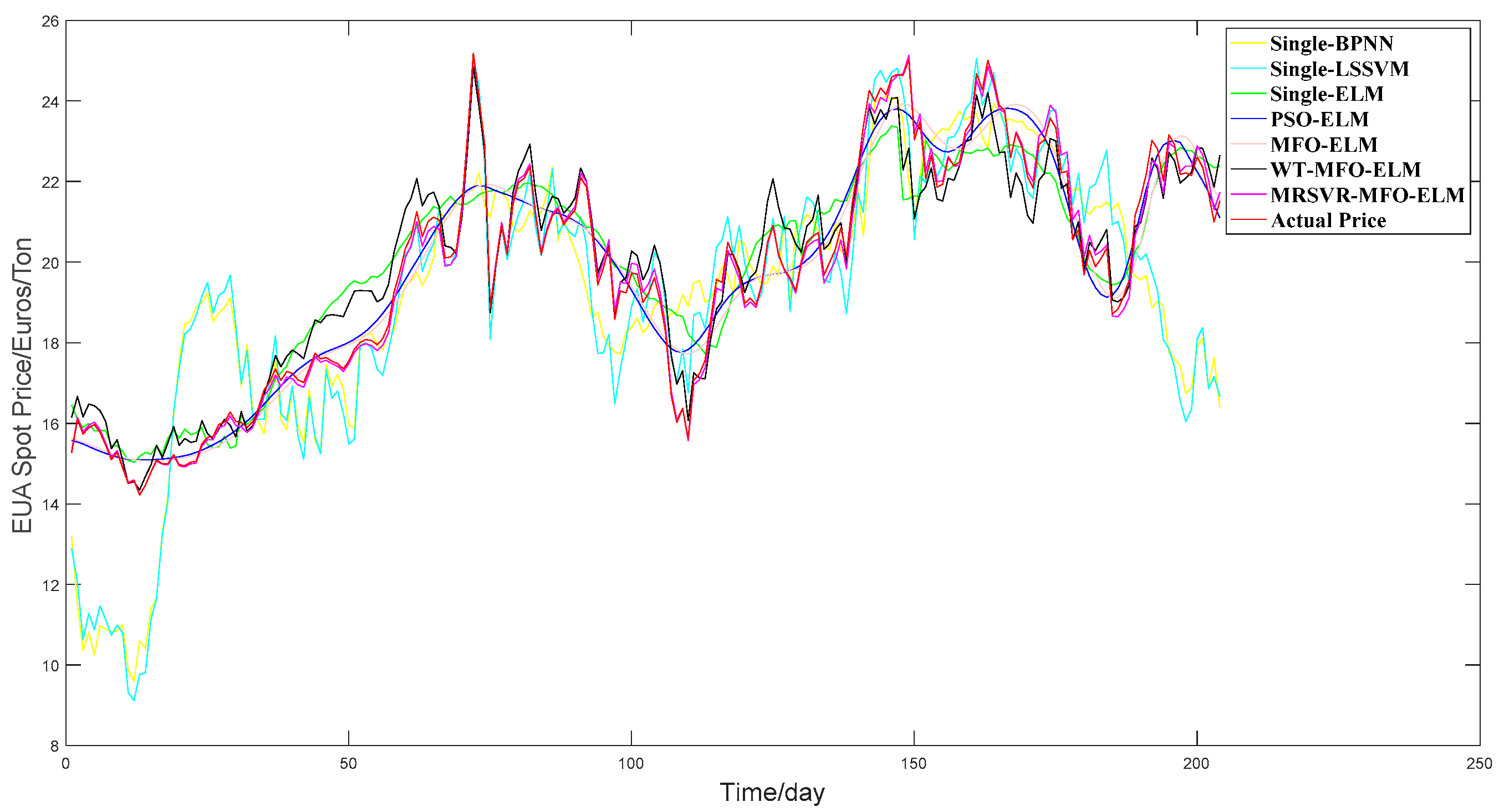
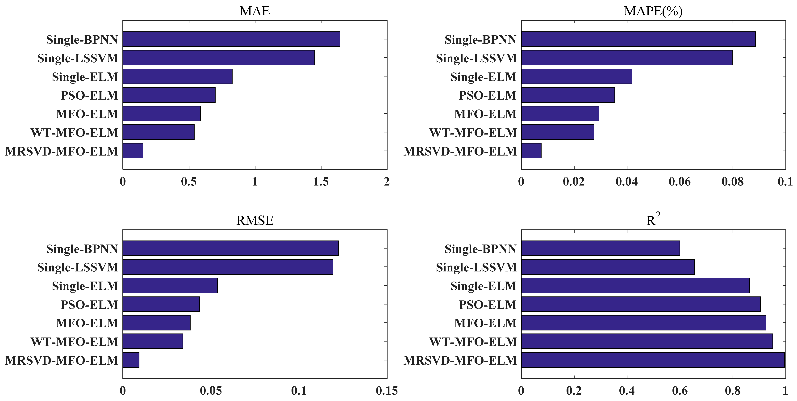
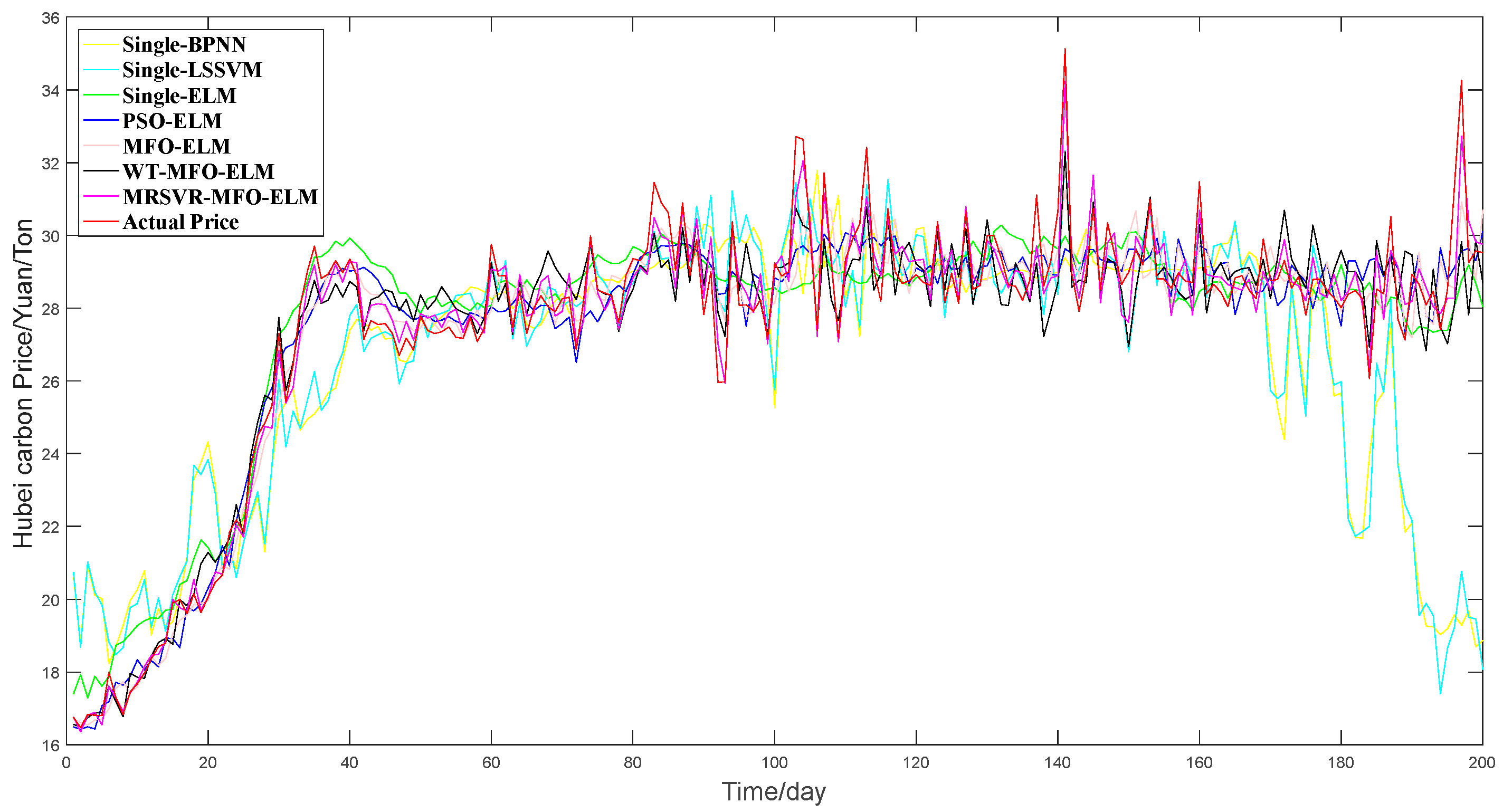
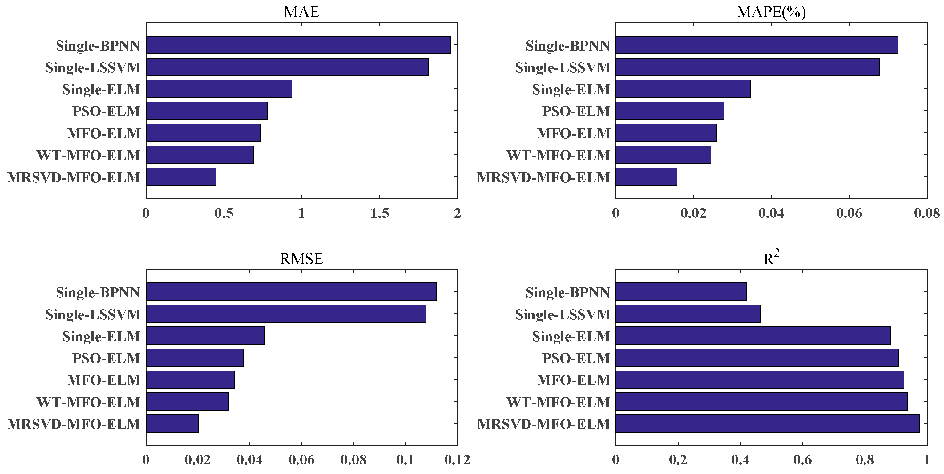
(b) Compared with WT-MFO-ELM, MFO-ELM, PSO-ELM, single ELM, single LSSVM, and single BPNN, the MRSVD-MFO-ELM model shows a clear strength in carbon price prediction results.

(c) ELM is a prediction model that is more suitable for carbon price forecasting than LSSVN and BPNN.

(d) ELM with an optimization algorithm is able to achieve better results than the ELM without optimization algorithms, and MFO performs better than the PSO in the optimization of ELM parameters.

(e) Decomposition methods help to improve prediction accuracy, and MRSVD presents superiority to WT in decomposing the carbon price.

This paper proposes a carbon price prediction model with high accuracy, to provide a scientific decision-making tool for carbon emission trading investors to comprehensively evaluate the value of carbon assets, avoid carbon market risks caused by carbon price changes and promote the stable and healthy development of carbon market.

By comparing the carbon prices of EU ETS and China ETS from 20 March 2018 to 20 March 2019, we find that the average value of the EUA spot price was 18.61 Euros per ton. However, the HUBEI carbon price was only 24.32 Yuan per ton, which was much lower than the EUA spot price. Therefore, China’s carbon market should take corresponding measures to reasonably price carbon assets. On the one hand, a reasonable carbon price can force enterprises to carry out low-carbon transformation more actively; on the other hand, it can attract more social capital to enter the carbon market and increase the market’s activity.

This paper primarily studied carbon price prediction, which takes consideration of energy price indicators, economic indicators, and historical carbon price sequences. In addition, there are many factors affecting carbon prices, such as policy, climate, carbon supply, and carbon market-related product prices. Therefore, there are still several directions to be studied.

References

1. Zhao, X.; Han, M.; Ding, L. Usefulness of economic and energy data at different frequencies for carbon price forecasting in the EU ETS. Appl. Energy 2018, 216, 132–141. [Google Scholar] [CrossRef]
2. Carnero, M.A.; Olmo, J.; Pascual, L. Modelling the Dynamics of Fuel and EU Allowance Prices during Phase 3 of the EU ETS. Energies 2018, 11, 3148. [Google Scholar] [CrossRef]
3. Chung, C.; Jeong, M.; Young, J. The Price Determinants of the EU Allowance in the EU Emissions Trading Scheme. Sustainability 2018, 10, 4009. [Google Scholar] [CrossRef]
4. Aatola, P.; Ollikainen, M.; Toppinen, A. Price determination in the EU ETS market: Theory and econometric analysis with market fundamentals. Energy Econ. 2013, 36, 380–395. [Google Scholar] [CrossRef]
5. Yu, J.; Mallory, M.L. Exchange rate effect on carbon credit price via energy markets. J. Int. Money Financ. 2014, 47, 145–161. [Google Scholar] [CrossRef]
6. Koch, N.; Fuss, S.; Grosjean, G.; Edenhofer, O. Causes of the EU ETS price drop: Recession, CDM, renewable policies or a bit of everything—New evidence. Energy Policy 2014, 73, 676–685. [Google Scholar] [CrossRef]
7. Alberola, É.; Chevallier, J.; Chèze, B. Price drivers and structural breaks in European carbon prices 2005–2007. Energy Policy 2008, 36, 787–797. [Google Scholar] [CrossRef]
8. Fan, J.H.; Todorova, N. Dynamics of China’s carbon prices in the pilot trading phase. Appl. Energy 2017, 208, 1452–1467. [Google Scholar] [CrossRef]
9. Zhu, B.Z.; Wei, Y.M. Carbon price forecasting with a novel hybrid ARIMA and least squares support vector machines methodology. Omega 2013, 41, 517–524. [Google Scholar] [CrossRef]
10. Na, W. Forecasting of Carbon Price Based on Boosting-ARMA Model. Stat. Inf. Forum 2017, 32, 28–34. [Google Scholar]
11. Byun, S.J.; Cho, H. Forecasting carbon futures volatility using GARCH models with energy volatilities. Energy Econ. 2013, 40, 207–221. [Google Scholar] [CrossRef]
12. Zeitlberger, A.C.; Brauneis, A. Modeling carbon spot and futures price returns with GARCH and Markov switching GARCH models Evidence from the first commitment period (2008–2012). Cent. Eur. J. Oper. Res. 2016, 24, 149–176. [Google Scholar] [CrossRef]
13. Guan, X.T. Research on Carbon Market Transaction Price Forecast Based on Grey Theory; Southwest Jiaotong University: Chengdu, China, 2016. [Google Scholar]
14. Chevallier, J. Nonparametric modeling of carbon prices. Energy Econ. 2011, 33, 1267–1282. [Google Scholar] [CrossRef]
15. Tsai, M.-T.; Kuo, Y.-T. A Forecasting System of Carbon Price in the Carbon Trading Markets Using Artificial Neural Network. Int. J. Environ. Sci. Dev. 2013, 4, 163–167. [Google Scholar] [CrossRef]
16. Zhang, J.; Li, D.; Hao, Y.; Tan, Z. A hybrid model using signal processing technology, econometric models and neural network for carbon spot price forecasting. J. Clean. Prod. 2018, 204, 958–964. [Google Scholar] [CrossRef]
17. Zhu, B.; Han, D.; Wang, P.; Wu, Z.; Zhang, T.; Wei, Y.-M. Forecasting carbon price using empirical mode decomposition and evolutionary least squares support vector regression. Appl. Energy 2017, 191, 521–530. [Google Scholar] [CrossRef]
18. Huang, G.B.; Zhu, Q.Y.; Siew, C.K. Extreme learning machine: A new learning scheme of feed forward neural networks. In Proceedings of the International Joint Conference on Neural Networks, Budapest, Hungary, 25–29 July 2004; pp. 985–990. [Google Scholar]
19. Li, S.; Goel, L.; Wang, P. An ensemble approach for short-term load forecasting by extreme learning machine. Appl. Energy 2016, 170, 22–29. [Google Scholar] [CrossRef]
20. Abdoos, A.A. A new intelligent method based on combination of VMD and ELM for short term wind power forecasting. Neurocomputing 2016, 203, 111–120. [Google Scholar] [CrossRef]
21. Shrivastava, N.A.; Panigrahi, B.K. A hybrid wavelet-ELM based short term price forecasting for electricity markets. Int. J. Electr. Power Energy Syst. 2014, 55, 41–50. [Google Scholar] [CrossRef]
22. Sun, W.; Wang, C.; Zhang, C. Factor analysis and forecasting of CO2 emissions in Hebei, using extreme learning machine based on particle swarm optimization. J. Clean. Prod. 2017, 162, 1095–1101. [Google Scholar] [CrossRef]
23. Mirjalili, S. Moth-flame optimization algorithm: A novel nature-inspired heuristic paradigm. Knowl. Based Syst. 2015, 89, 228–249. [Google Scholar] [CrossRef]
24. Mei, R.N.S.; Sulaiman, M.H.; Mustaffa, Z.; Daniyal, H. Optimal reactive power dispatch solution by loss minimization using moth-flame optimization technique. Appl. Soft Comput. 2017, 59, 210–222. [Google Scholar]
25. Elsakaan, A.A.; El-Sehiemy, R.A.; Kaddah, S.S.; Elsaid, M.I. An enhanced moth-flame optimizer for solving non-smooth economic dispatch problems with emissions. Energy 2018, 157, 1063–1078. [Google Scholar] [CrossRef]
26. Tan, Z.; Zhang, J.; Wang, J.; Xu, J. Day-ahead electricity price forecasting using wavelet transform combined with ARIMA and GARCH models. Appl. Energy 2010, 87, 3606–3610. [Google Scholar] [CrossRef]
27. Wei, S.; Chongchong, Z.; Cuiping, S. Carbon pricing prediction based on wavelet transform and K-ELM optimized by bat optimization algorithm in China ETS: The case of Shanghai and Hubei carbon markets. Carbon Manag. 2018, 9, 605–617. [Google Scholar] [CrossRef]
28. Wang, Y.-H.; Yeh, C.-H.; Young, H.-W.V.; Hu, K.; Lo, M.-T. On the computational complexity of the empirical mode decomposition algorithm. Phys. A Stat. Mech. Appl. 2014, 400, 159–167. [Google Scholar] [CrossRef]
29. Wang, S.; Zhang, N.; Wu, L.; Wang, Y. Wind speed forecasting based on the hybrid ensemble empirical mode decomposition and GA-BP neural network method. Renew. Energy 2016, 94, 629–636. [Google Scholar] [CrossRef]
30. Abu-Shikhah, N.; Elkarmi, F. Medium-term electric load forecasting using singular value decomposition. Energy 2011, 36, 4259–4271. [Google Scholar] [CrossRef]
31. Bhatnagar, G.; Saha, A.; Wu, Q.J.; Atrey, P.K. Analysis and extension of multiresolution singular value decomposition. Inf. Sci. 2014, 277, 247–262. [Google Scholar] [CrossRef]
32. Zhao, G.; Xu, L.; Gardoni, P.; Xie, L. A new method of deriving the acceleration and displacement design spectra of pulse-like ground motions based on the wavelet multi-resolution analysis. Soil Dyn. Earthq. Eng. 2019, 119, 1–10. [Google Scholar] [CrossRef]
33. Yue, Y.; Jiang, T.; Han, C.; Wang, J.; Chao, Y.; Zhou, Q. Suppression of periodic interference during tunnel seismic predictions via the Hankel-SVD-ICA method. J. Appl. Geophys. 2019, 168, 107–117. [Google Scholar] [CrossRef]
34. Zhou, K.; Li, M.; Li, Y.; Xie, M.; Huang, Y. An Improved Denoising Method for Partial Discharge Signals Contaminated by White Noise Based on Adaptive Short-Time Singular Value Decomposition. Energies 2019, 12, 3465. [Google Scholar] [CrossRef]
35. Sha, H.; Mei, F.; Zhang, C.; Pan, Y.; Zheng, J. Identification Method for Voltage Sags Based on K-means-Singular Value Decomposition and Least Squares Support Vector Machine. Energies 2019, 12, 1037. [Google Scholar] [CrossRef] [Green Version]
36. Sheng, H.; Li, C.; Wang, H.; Yan, Z.; Xiong, Y.; Cao, Z.; Kuang, Q. Parameters Extraction of Photovoltaic Models Using an Improved Moth-Flame Optimization. Energies 2019, 12, 3527. [Google Scholar] [CrossRef] [Green Version]
37. Xu, Y.; Chen, H.; Heidari, A.A.; Luo, J.; Zhang, Q.; Zhao, X.; Li, C. An efficient chaotic mutative moth-flame-inspired optimizer for global optimization tasks. Expert Syst. Appl. 2019, 129, 135–155. [Google Scholar] [CrossRef]
38. Liu, X.; Yang, L.; Zhang, X.; Wang, L. A Model to Predict Crosscut Stress Based on an Improved Extreme Learning Machine Algorithm. Energies 2019, 12, 896. [Google Scholar] [CrossRef] [Green Version]
39. Li, N.; He, F.; Ma, W. Wind Power Prediction Based on Extreme Learning Machine with Kernel Mean p-Power Error Loss. Energies 2019, 12, 673. [Google Scholar] [CrossRef] [Green Version]
40. EUA Spot Price, DEC19 Price, DEC20 Price, DEC21 Price, EUA Spot Trading Volume. Available online: https://www.eex.com/en/ (accessed on 21 March 2019).
41. CSX Coal Future Price. Available online: https://www.theice.com/market-data (accessed on 21 March 2019).
42. Crude Oil Future Price, Natural Gas Future Price. Available online: https://www.eia.gov/ (accessed on 21 March 2019).
43. Euro Stoxx 50, Shanghai Composite Index. Available online: https://cn.investing.com/ (accessed on 19 April 2019).
44. Qi, S.; Wang, B.; Zhang, J. Policy design of the Hubei ETS pilot in China. Energy Policy 2014, 75, 31–38. [Google Scholar] [CrossRef]
45. Hubei Carbon Price. Available online: http://www.tanjiaoyi.com/ (accessed on 19 April 2019).
Figure 1. The decomposition process of multi-resolution singular value decomposition (MRSVD).
Energies 12 04283 g001
Figure 2. The flowchart of the carbon price forecasting model.
Energies 12 04283 g002
Figure 3. The comparison framework of the carbon price forecasting model.
Energies 12 04283 g003
Figure 4. The original carbon price under the European Union emissions trading scheme (EU ETS).
Energies 12 04283 g004
Figure 5. The curves of European emission allowances (EUA) spot trading volume and its external factors.
Energies 12 04283 g005
Figure 6. The flowchart of external factor selection.
Energies 12 04283 g006
Figure 7. Decomposed results of EUA spot price by wavelet transform (WT).
Energies 12 04283 g007
Figure 8. Decomposed results of EUA spot price by MRSVD.
Energies 12 04283 g008
Figure 9. The partial autocorrelation function (PCAF) results of the EUA spot price after WT.
Energies 12 04283 g009
Figure 10. The PCAF results of the EUA spot price after MRSVD.
Energies 12 04283 g010
Figure 11. The convergence curve of the moth–flame optimization (MFO).
Energies 12 04283 g011
Figure 12. The fitting curves of seven models for EUA spot price forecasting.
Energies 12 04283 g012
Figure 13. Evaluation criteria values of seven models for EUA spot price forecasting.
Energies 12 04283 g013
Figure 14. The PCAF results of Hubei carbon price after WT.
Energies 12 04283 g014
Figure 15. The PCAF results of Hubei carbon price after MRSVD.
Energies 12 04283 g015
Figure 16. The fitting curves of seven models for Hubei carbon price forecasting.
Energies 12 04283 g016
Figure 17. Evaluation criteria values of seven models for Hubei carbon price forecasting.
Energies 12 04283 g017