Article

Wake of a Ducted Vertical Axis Tidal Turbine in Turbulent Flows, LBM Actuator-Line Approach

1
Normandie Univ, UNICAEN LUSAC, EA 4253, 60 rue Max-Pol Fouchet, CS 20082 Cherbourg, France
2
Conservatoire National des Arts et Métiers-INTECHMER, Bd de Collignon, 50110 Tourlaville, France
*
Author to whom correspondence should be addressed.
Energies 2019, 12(22), 4273; https://doi.org/10.3390/en12224273
Submission received: 3 October 2019 / Revised: 29 October 2019 / Accepted: 6 November 2019 / Published: 9 November 2019
(This article belongs to the Section A3: Wind, Wave and Tidal Energy)

Abstract

:
Vertical axis tidal turbines are devices that extract the kinetic energy from tidal currents. Tidal currents can be highly turbulent. Since ambient turbulence affects the turbine hydrodynamic, it is critical to understand its influence in order to optimize tidal farms. Actuator Line Model (ALM) combined with Large Eddy Simulation (LES) is a promising way to comprehend this phenomenon. In this article, an ALM was implemented into a Lattice Boltzmann Method (LBM) LES solver. This implementation gives good results for predicting the wake of a vertical axis tidal turbine placed into a turbulent boundary layer. The validated numerical configuration was then used to compute the wake of a real size ducted vertical axis tidal turbine. Several upstream turbulence rates were simulated. It was found that the shape of the wake is strongly influenced by the ambient turbulence. The cost-to-precision ratio of ALM-LBM-LES compared to fully resolved LBM-LES makes it a promising way of modeling tidal farms.

Graphical Abstract

1. Introduction

In the context of the global energy crisis, developing renewable energies is of primal importance. Among the renewable resources available are tidal currents. Tidal currents can be exploited with tidal turbines. Tidal turbines extract the kinetic energy contained in tidal currents, mostly in areas where maximum currents are over 1.5 m.s 1 [1]. There are numerous technologies for tidal turbines and most of them can be classified into two categories: the horizontal axis and the vertical axis. This work is realized in collaboration with Hydroquest (Figure 1), a vertical axis tidal turbines manufacturer. Thus, this paper investigates the behavior of vertical axis tidal turbines. Most tidal sites are characterized by strong turbulence intensities [2]. Several test campaigns have already been performed, such as in the sound of Islay where the turbulence intensity was found to be between 9.5 % and 10.3 % [3] or in the Grand Passage where the turbulence intensity was found to be between 10 % and 20 % [4]. The presence of turbulence in most tidal sites has led companies and academics to study the effects of ambient turbulence over tidal turbines. Mycek et al. [5] carried out such study for a horizontal axis tidal turbine model. They showed that going from 3 % to 15 % turbulence intensity decreases the power coefficient by a maximum of 10 % . It also reduces the wake recovery by more than 5 D . Tidal turbines will most likely be installed into farms. The results from Mycek et al. show that interactions between turbulence and tidal turbines will directly affect the layout and performances of farms. Predicting those interactions is thus crucial for reducing the cost of tidal farms.
Several studies of vertical axis tidal turbines have been conducted during the past few years. Recently, Ouro et al. [6] carried out an experimental study of a vertical axis tidal turbine model in a turbulent flow with approximately 15 % turbulence intensity for the streamwise velocity. They have highlighted different regions of the wake and the persistence of the turbine footprint up to 14 D . Hochman et al. [7] studied the impact of the presence of an atmospheric boundary layer on vertical axis wind turbine model. They showed that there is little impact of the atmospheric boundary layer on the turbine. However, little is known about the impact of several turbulent inflow conditions over a single real size tidal turbine.
Vertical axis tidal turbines are home to complex phenomena such as dynamic stall. During a revolution of the rotor, the blade of a vertical axis turbine have an oscillating angle of attack that passes through a maximum positive value and a minimum negative value. At a low enough tip-speed ratio, the angle of attack can be superior to the static stall angle. The main effect of the dynamic stall is to delay the stall, thus increasing the performance of the turbine. It is therefore important to consider the dynamic stall when studying vertical axis tidal turbine. The downstream half of the blade trajectory is located in the wake of the upstream half. Thus, there is a strong asymmetry between the upstream half and the downstream half. Brochier et al. [8] showed how vortex shedding occurs during the rotation of the blades and how it affects the right/left symmetry. Ouro et al. [9] proposed a Large Eddy Simulation (LES) geometry resolved study of a vertical axis tidal turbine. They showed the vortex shedding strong dependence on tip-speed ratio and how it affects the hydrodynamic of the turbine.
Experimental studies are limited to turbine models and thus suffer from scale effects. In situ measurement are still expensive and difficult to acquire. Blade-resolved Computational Fluid Dynamics (CFD) approaches are appropriate to study vertical axis tidal turbines [9]. Because the hydrodynamic of vertical axis tidal turbines is highly unsteady, LES are well adapted here [9]. LES computational cost is still prohibitive for real size tidal turbine [10] and simplified approaches are preferred solutions. Shamsoddin and Porté-Agel [11] showed that Actuator Line Model (ALM) LES is more appropriate than Actuator Cylinder LES for modeling vertical axis turbine. Liu et al. [12] modeled a horizontal axis tidal turbine model and showed that ALM-LES is well suited for modeling tidal turbine in different turbulent conditions.
This paper proposes the study of a ducted three-bladed H-type Darrieus contra-rotating vertical axis tidal turbine. This study was carried out with a Lattice Boltzmann Method (LBM) ALM LES approach. The LBM is a highly parallelizable unsteady CFD method [13]. Since it has a low numerical dissipation [14], it is well suited for propagating the wake of tidal turbines. The actuator line model used considers dynamic stall effect. Four upstream turbulence intensities were simulated. The chosen turbulence intensities are 0 % , 4 % , 8 % and 12 % . The main goal of this study was to highlight the effects of several turbulence rates on a single vertical axis tidal turbine, thus providing a better understanding to tidal turbines manufacturers. This work is divided into three sections, after this Introduction. Section 2 gives elements on the theoretical background of the approach. Since this approach has not been validated yet, validation elements are also presented in this section. Section 3 presents the results of ALM-LBM simulations of the vertical axis turbine. Section 4 gives the conclusions and prospects of this work.

2. Materials and Methods

This section is divided into four subsections. Section 2.1 succinctly presents the LBM models used. Section 2.2 introduces the implemented ALM model. Then, the approach is validated with an experimental case in Section 2.3. Section 2.4 is dedicated to the real-size turbine simulation set-up.

2.1. The Lattice Boltzmann Method

The LBM is an unsteady CFD method based on the Lattice Gas Automata and the Boltzmann equation [13]. The LBM solver used here is the open-source library Palabos [15], developed at the University of Geneva. LBM describes the fluid from a molecular point of view through distribution functions f. Distribution functions represent the density of molecules at a certain location in space with a given velocity. Thus, it is a continuous function of space, time and velocity. Space is discretized into a Cartesian grid, or lattice, with a grid spacing Δ x . Cartesian grids in Palabos can be divided into several levels, by a factor 2 in mesh size and time step between two adjacent levels. This multi-block approach was described by Lagrava et al. [16].
Velocity space in Palabos is discretized by defining a finite set of directions of propagation. At each lattice node lies n distribution functions f i , each representing the density of molecules going in a direction. The set used in this article is the D 3 Q 27 set with 27 directions of propagation, where 3 stands for three dimensions. Time in LBM is discretized into constant time steps Δ t . The fluid behavior is resolved into two steps, the collision step and the streaming step. The collision step is calculated with Equation (1):
f i ( x , t ) = Ω ( f i ( x , t ) ) ,
where Ω is the collision operator and f i are the post-collision distribution functions. The collision operator represents the collision between molecules and is the core of the method. There are many collision operators available in Palabos and even more in the literature. The collision operator used in this paper is a regularized BGK collision operator. It was described by Malaspinas [17] and was chosen for its stability [17]. The collision operator used allows fluid forcing. Indeed, an external force is needed for implementing the actuator line model. The streaming step consists in the propagation of distribution functions onto the neighboring nodes pointed by the discrete directions of propagation. It is calculated with Equation (2):
f i ( x + c i Δ t , t + Δ t ) = f i ( x , t ) ) ,
where c i are the directions of propagation and Δ t is the time step. To reduce the mesh size, a LES model is used. It is a static Smagorinsky model and was described by Malaspinas and Sagaut [18]. Following the work of Shamsoddin and Porté-Agel [11], we chose C s = 0.1 .
All the boundary conditions used are based on a second-order accurate finite-difference scheme described by Skordos [19] and Latt et al. [20]. It was chosen because of its stability at high Reynolds number [20]. For generating the inflow turbulence, a Divergence Free Synthetic Eddy Method (DFSEM) [21] was implemented by Palabos, Grondeau et al. [22]. To increase the numerical stability of simulations, viscous damping zones are placed on the side boundaries and on the outlet.

2.2. Actuator Line Model

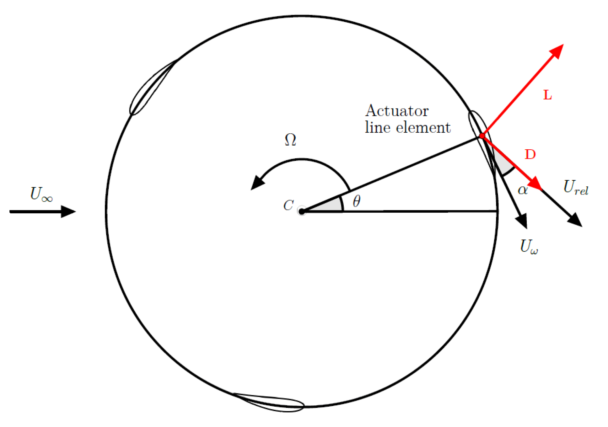
Since it was not present in Palabos, an actuator line model was implemented. The chosen model is a modified MIT dynamic stall model, which was described in detail by Shamsoddin and Porté-Agel [23]. This latter approach has been slightly modified. In their article, the averaged angle of attack α f i t is generated with an eighth-order polynomial. In this study, it is generated with a cubic spline in order to better capture the evolution of the angle of attack. Actuator Line Models, introduced by Shen and Sørensen [24], represent the blades with a force f A L computed from the airfoil tabulated C L and C D . The dynamic stall model acts on those two coefficients and has a non-negligible influence [11]. The blades of the turbine are simplified into lines, which are discretized into a number of elements (Figure 2). The force f A L is applied to the fluid at the location of these elements and is calculated with Equation (3).
f A L ρ = ( c Δ l ) ( U r e l 2 2 ) ( C L D S e L + C D D S e D ) ,
where c is the chord of the blade, Δ l is the spacing between elements and U r e l is the norm of the relative velocity of the blade. Spacing Δ l is equal to the mesh size at the turbine location. C L D S and C D D S are the lift and drag coefficients, respectively, modified by the dynamic stall algorithm described in [23]. e L is the lift unit vector and e D is the drag unit vector. The relative velocity is calculated with Equation (4):
U r e l = ( U f l u i d . N ) N + ( U f l u i d . T U ω ) T ,
where U ω = ω R R , with R the radius of the rotor and ω R its rotational speed. U f l u i d is the fluid velocity calculated at the element location. The vector N is normal to the blade displacement and the vector T is tangent to the blade displacement. The angle of attack α is calculated with Equation (5):
α = t a n 1 U f l u i d . N U f l u i d . T U ω .
The actuator line moves at the rotational speed of the rotor ω R at each lattice iteration. Shamsoddin et al. [11] applied the force on a single node of the mesh. To avoid numerical instabilities, the force is distributed around each element of the actuator line. The distribution kernel is η ( ϵ , d ) and is given in Equation (6):
η ( ϵ , d ) = 1 ϵ 3 π 3 / 2 e x p d ϵ 2 ,
where d is the distance between a node of the lattice and an actuator line element. Studies about the choice of the ϵ parameter already exist. Some studies suggest choosing ϵ = 4 Δ x [25,26], where Δ x is the mesh size at the turbine location. In Palabos, the domain is divided into cuboids of n × n × n nodes; here, n = 14 . Those cuboids are then distributed as equally as possible between the processors. To do non-local operations, the nodes surrounding a cuboid need to be loaded with it, thus degrading the efficiency. To keep the efficiency of Palabos and stay as local as possible, a compromised between the methods of Bachant et al. [25] and Shamsoddin and Porté-Agel [11] is made and we chose ϵ = 2 Δ x . The same ϵ value was chosen by Liu et al. [12] for modeling a horizontal axis tidal turbine. The force applied to lattice nodes is calculated with Equation (7):
f A L ( x ) = η ( ϵ , d ) f A L .

2.3. Accuracy of the Model

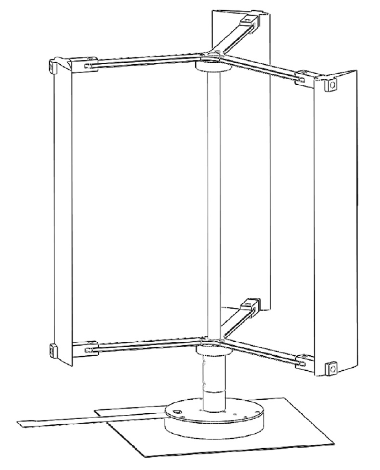
The code was validated with the experimental results from Rolin and Porté-Agel [27]. The case consists in a three-bladed vertical axis wind turbine placed in a turbulent boundary layer. The rotor characteristics are given in Table 1 and the turbine is illustrated in Figure 3. The blades are straight and their profile is a NACA0018. The wind tunnel is 28.00 m long, 2.57 m wide and 2.00 m tall. The turbine is located 20.00 m downstream of the tunnel contraction such that the turbulent boundary layer is fully developed [27]. The turbine half-height is located 0.13 m above the ground. The reference velocity is the axial velocity at the turbine mid-height, U H / 2 = 9.43 m.s 1 .
The turbine was modeled with the ALM dynamic-stall model presented in Section 2.2. Tabulated C L and C D were taken from Kumar et al. [28] for low angles of attack (inferior to 25 ) and from Sheldahl and Klimas [29] for high angles of attack [11]. The mast of the turbine has a radius of approximately 4 × 10 3 m and it is also modeled with a force. Its drag coefficient is 1. The H-bars are also modeled with a force. Their length is approximately 7 × 10 3 m, their lift is neglected, and they have a drag of 0.05 , estimated with a 2 D k ω URANS simulation.
The upstream velocity profiles are generated with a DFSEM boundary condition. The DFSEM, based on the SEM of Jarrin et al. [30], was introduced by Poletto et al. [21]. It generates a random upstream turbulence that respects a prescribed Reynolds tensor. Input parameters of the DFSEM are the average axial velocity profile, the average Reynolds tensor profile, the size of the DFSEM eddies and the number of DFSEM eddies. Upstream average axial velocity and fluctuations were extracted from Rolin and Porté-Agel [27]. The Reynolds tensor is symmetric and all its diagonal components are equal to the axial velocity fluctuations. Eddies are spherical and their diameter is 0.15 m. The number of eddies is set to have an eddy density of 2.0 . The eddy density is defined as the ratio between the volume of eddies and the volume of the DFSEM domain [21]. The top and side boundary conditions are velocity-imposed boundary conditions set to match the prescribed inflow velocity profile. The outlet is a pressure-imposed boundary condition. The bottom boundary condition is a velocity-imposed boundary condition modified with a wall law, based on the formulation of Spalding [31].
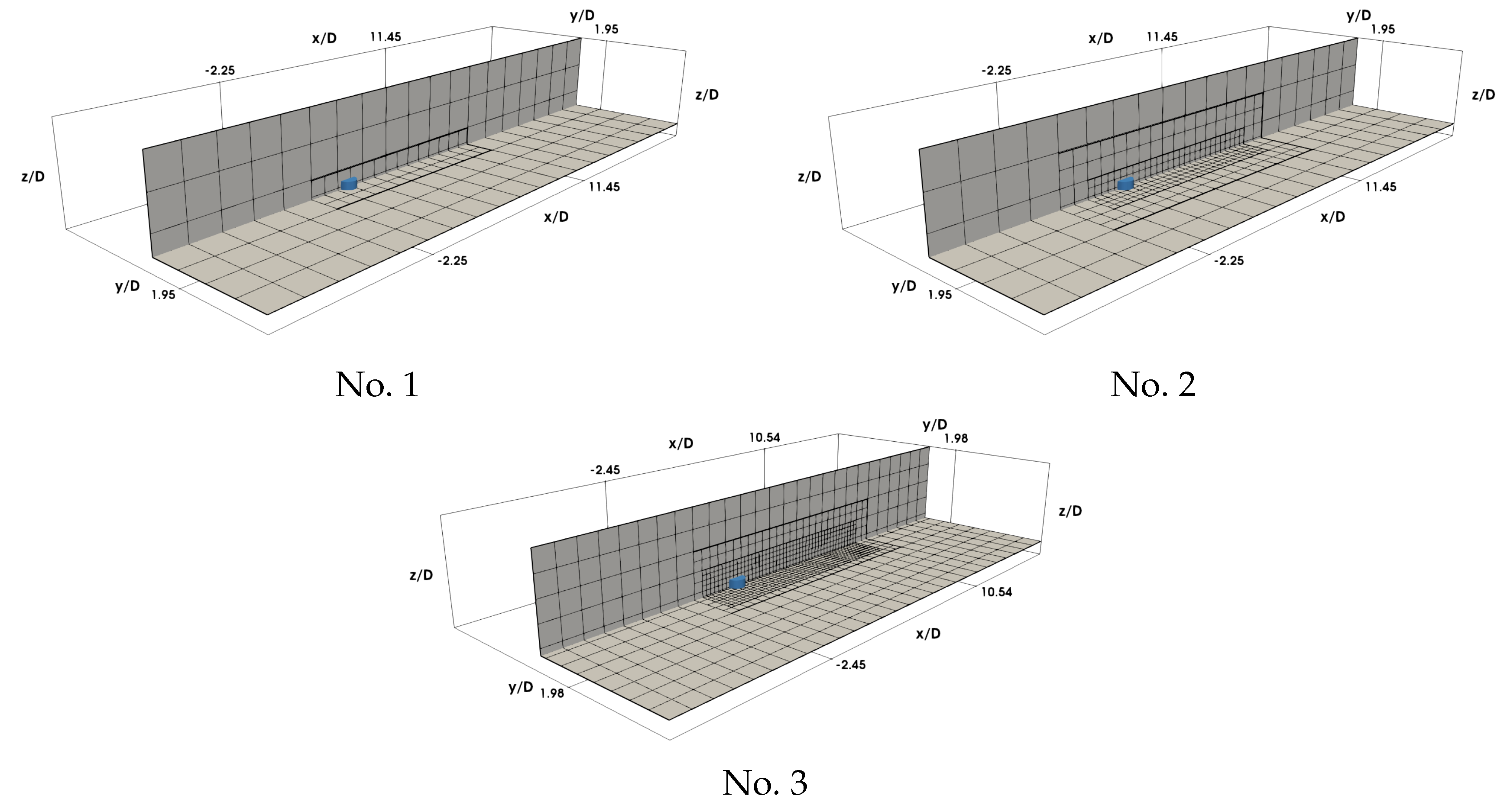
Computational domain dimensions were set to match the wind tunnel dimensions, except for the length. The computational domain is 6 m long and the turbine is located 12 D downstream of the inlet. Because the distribution kernel parameter ϵ varies with the mesh size Δ x , three mesh sizes were tested to evaluate the influence of both mesh size and distribution kernel. The LBM is a weakly compressible method. The time step was set to keep the Mach number identical in all cases, Ma m a x 0.08 . Table 2 summarizes the various meshes, visible in Figure 4. Simulations were carried out at CRIANN [32] (France) on Broadwell CPU cores ( 2.4 GHz).
U D e f = 1 < U x > / U H / 2
U x * = < U x > / U H / 2
T K E + = T K E W T K E 0
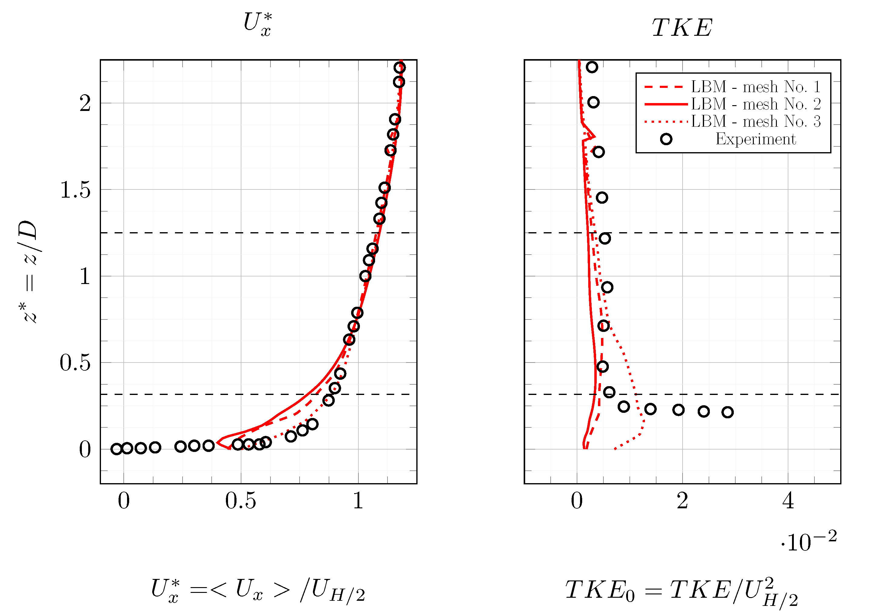
Three wake quantities were investigated. The average axial velocity deficit is defined in Equation (8), where < U x > is the time-averaged axial velocity. The dimensionless average axial velocity is calculated with Equation (9). The dimensionless turbulent kinetic energy (TKE) is defined in Equation (10), where T K E W is the T K E calculated in the wake and T K E 0 is the T K E calculated upstream of the turbine. Both T K E are divided by U H / 2 2 . Figure 5 shows the location of the turbine and the plane where the statistics are calculated. The convergence lasted 70 rotations and data were averaged over 60 rotations of the turbine. An additional plane was extracted 2.0 D upstream of the turbine to evaluate differences between the experimental flow and the numerical flow (Figure 6). LBM average axial velocity profiles are close to experimental profiles. Differences are observed in the ground vicinity. Indeed, the wall law does not allow predicting the proper flow behavior in the viscous sub-layer. Similarly, high differences are observed on the T K E in this area. The mesh resolution does not allow for a proper turbulence production. The turbulence generated by the DFSEM close to the bottom is not propagated on a long enough distance and, in lack of production, it is dissipated. Above the flume bottom, T K E profiles from the ALM-LBM simulations are close to the experimental one. The small T K E peak observed at z / D = 1.8 comes from the influence of the mesh interface between two levels of the mesh.
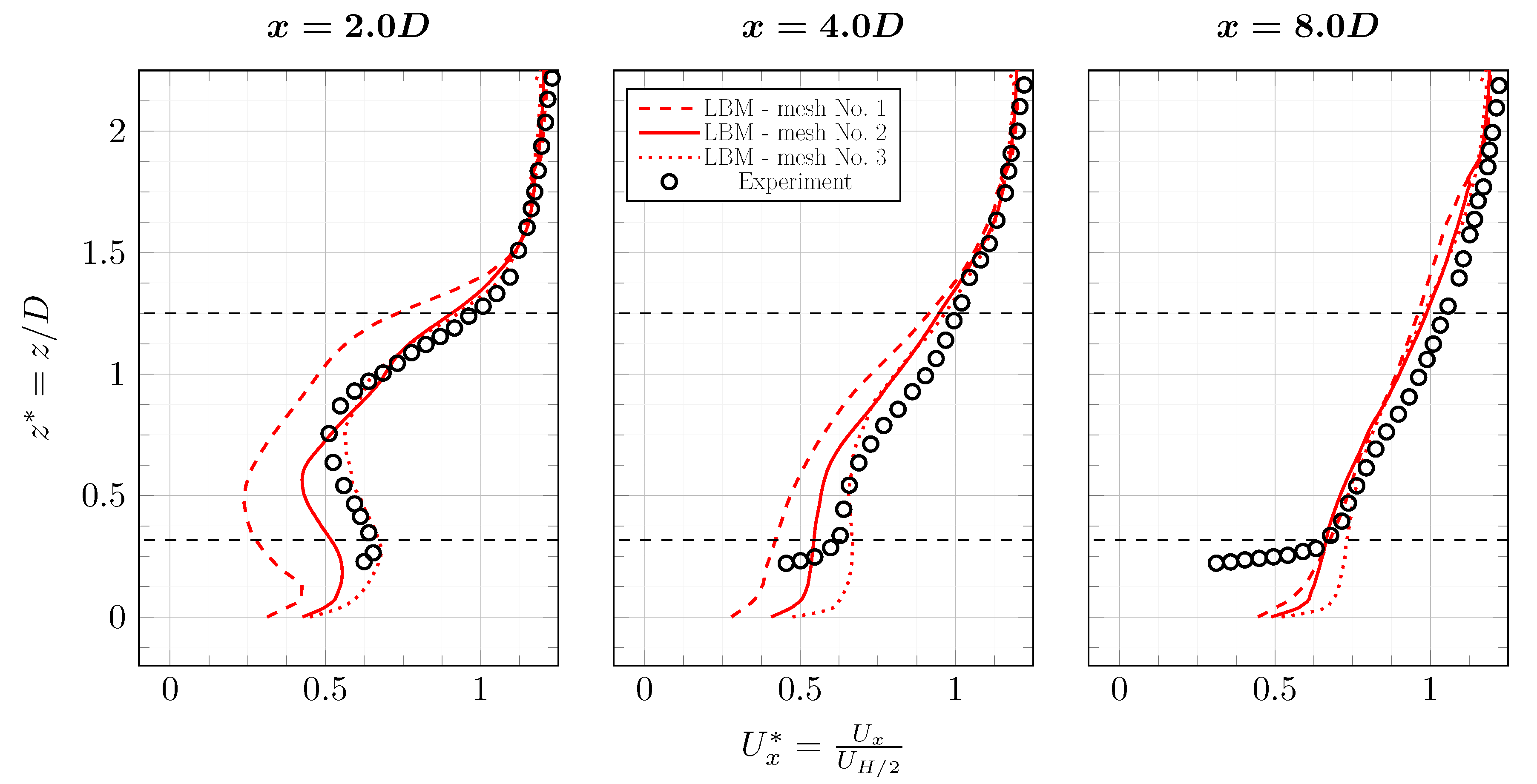
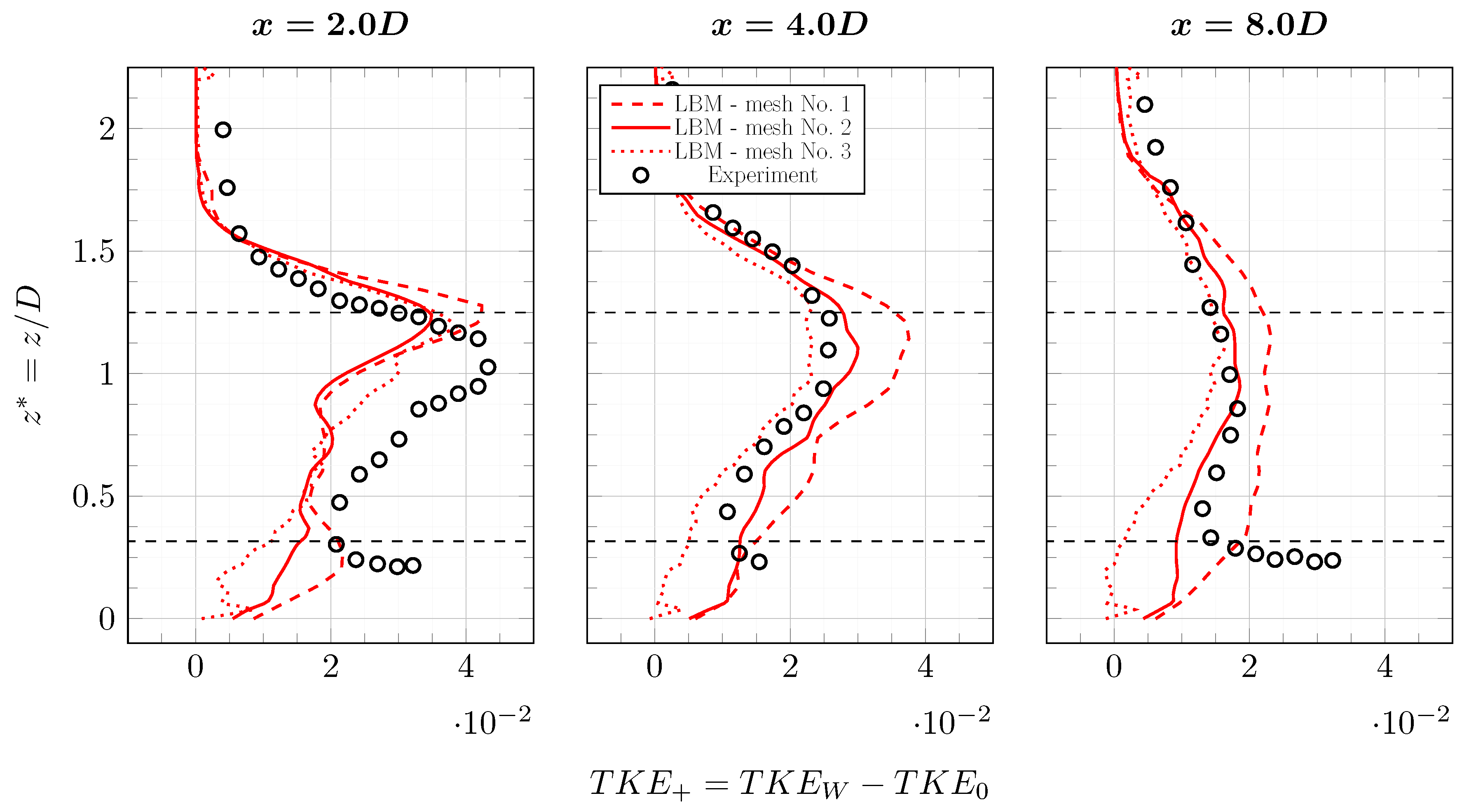
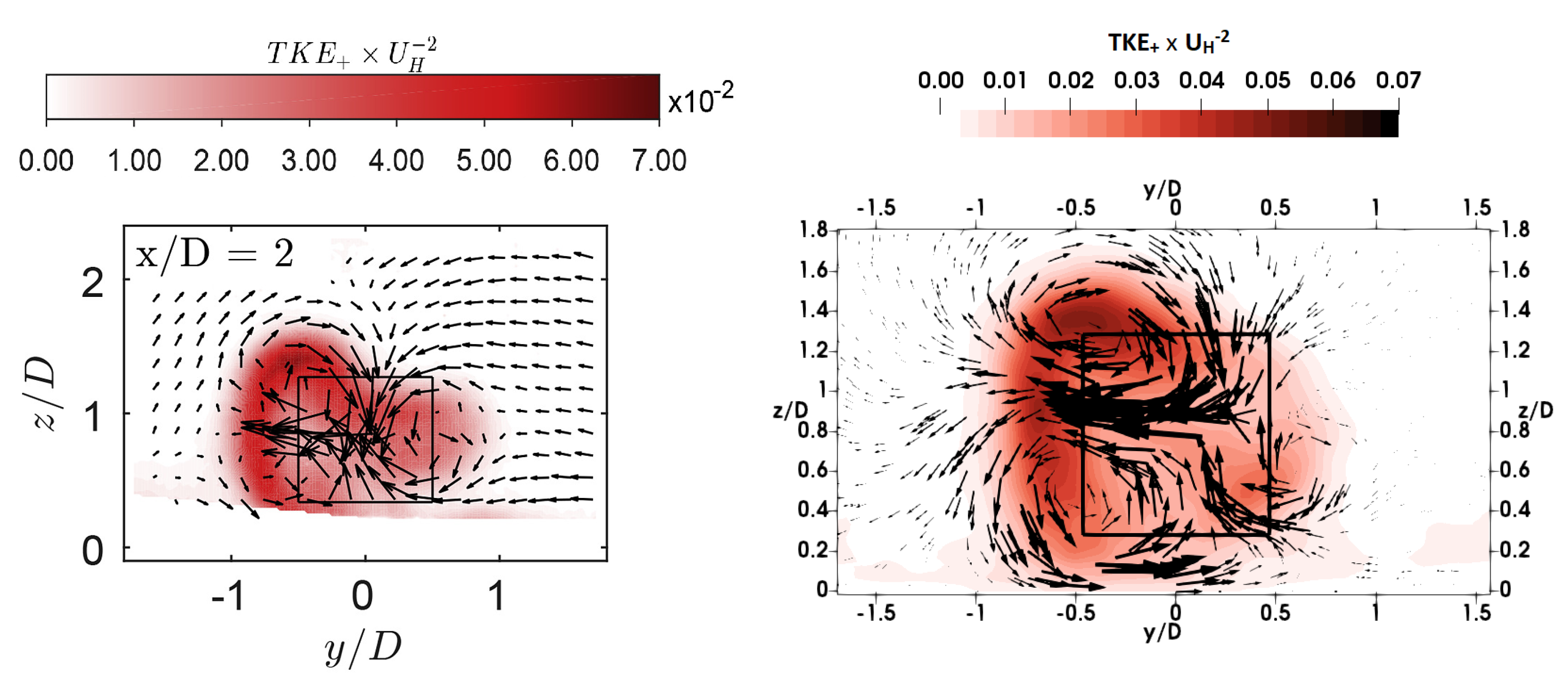
Figure 7 shows the average axial velocity deficit in the wake of the turbine and Figure 8 the average axial velocity. The maximum velocity deficit at 2.0 D is different for the three meshes. The velocity deficit for Mesh No. 3 is too small compared to the experimental one. This difference tends to disappear after 4.0 D and the maximum velocity deficit is correctly predicted. The only difference that persist in the far wake is the asymmetry of the profile in Figure 7. It is more pronounced on the experimental profile than on the simulation profiles. Figure 9 and Figure 10 show the average TKE in the wake of the turbine. The asymmetry difference can be observed in Figure 9. The ALM model is functioning with a wide angle of attack range (between −60 and 60 ) because of the low tip-speed ratio. This could induce some discrepancies. Figure 11 shows the contour of T K E + in a plane 2.0 D downstream of the turbine. In-plane velocity vectors are also plotted. Two contra-rotating vortices in the negative y side are identified in both the experimental and simulation results. Further away in the wake, 6.0 D downstream of the turbine, the bottom vortex is no longer visible in the experimental plane (Figure 12) while it is still there in the simulation. In the experiment, the bottom vortex vanishes because of the turbulent boundary layer. In the simulations, because the turbulence is not energetic enough close to the flume bottom, the contra-rotating vortices pair is conserved. This difference in wake structure could also induce the discrepancies observed on the wake asymmetry. Vertical profiles plotted in Figure 8 and Figure 10 are relatively close to experimental profiles. Only differences close to the bottom persist. Errors of the LBM-LES simulations are given in Table 3. Mesh No. 2 gives the best results overall. It is surprising to find out that it is not Mesh No. 3. In Section 2.2, it is explained that the ϵ parameter depends on the mesh size and is equal to ϵ = 2 Δ x . Therefore, the distribution volume for Mesh No. 3 is rather small compared to the blade chord. This could explain the differences for Mesh No. 3. It would be interesting to increase the distribution parameter ϵ as the mesh size decreases, but for reasons of efficiency, it is not possible to do so at this time.
Mesh No. 2 gives relatively good wake prediction both for shapes and quantities. The configuration with Δ x = D / 30 was kept for modeling the real-size tidal turbine. Most of the differences observed between the experiment and the simulations probably come from the low mesh resolution close to the bottom of the flume. Resolving the flow in this area would cost a lot of computational resources and is not adapted to simplified approaches such as ALM. Since the real-size turbine will not be as close to the viscous sublayer as the turbine from Rolin et al. [27], its influence should not be as significant.

2.4. Turbine Set-Up

The turbine studied here has the same design as the Hydroquest turbine in Figure 1. The turbine has four rotors. The top rotors are shifted by 60 degrees compared to the bottom rotors. The left and right rotors are contra-rotating. Rotors are H-type Darrieus with straight blades. Blades chord and profile are confidential. Tabulated C L and C D are obtained with XFLR5 software with N c r i t = 9 and 300 panels. Table 4 summarizes the rotors characteristics. The tip-speed ratio λ is chosen close to the operating point of the turbine, λ = 1.5 .
Rotors axis and H-bars are modeled with actuator lines. As for the blades, forces from axis and H-bars are distributed around the actuator lines elements. The stator is modeled with an off-lattice approach, described in Guo et al. [33]. A no-slip boundary condition or a wall model would require an unaffordable fine mesh considering the Reynolds numbers at stake. A free-slip condition is used to model the interactions between rotors and stator. The off-lattice algorithm is set to impose a free-slip boundary condition on the stator walls. The bottom of the stator is located 5 m above the sea-bed. Figure 13 is an illustration of the geometry used for the LBM-ALM simulations. The stator is approximately 11 m high, 25 m wide and 10 m long. The equivalent diameter D e q is equal to the turbine width, D e q = 25.0 m.
The inflow velocity profiles are generated with a DFSEM boundary condition. The average axial velocity profile is constructed with the power law given in Equation (11):
U x ( z ) = U x δ z δ 1 n ,
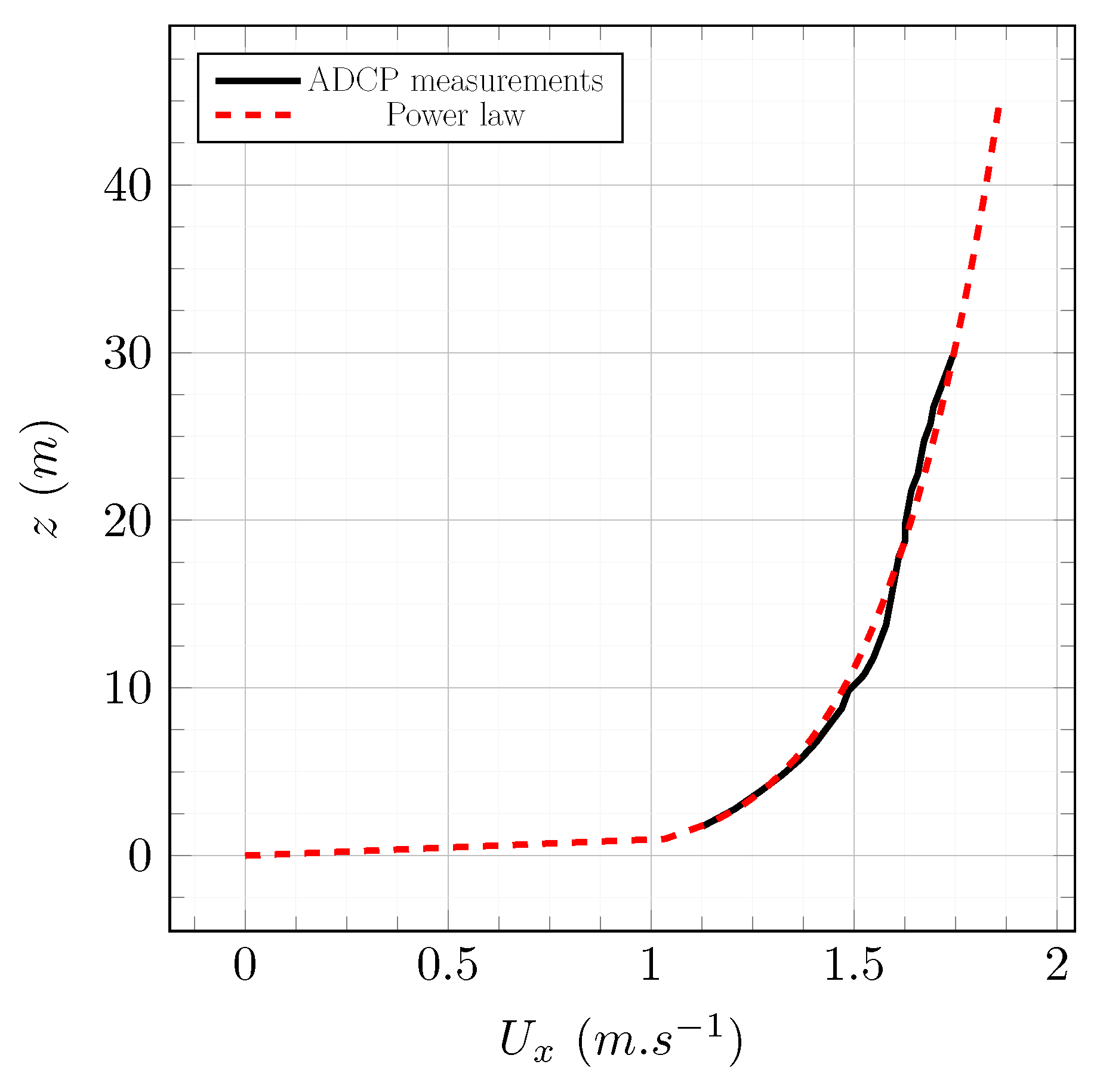
where U x δ is the axial velocity at height δ and z is the distance from the sea-bed. For the simulations presented afterwards, δ is equal to 10.0 m and U x δ = 1.475 m . s 1 . The parameter n depends on the flow. Here, n = 6.5 was chosen, relatively to the velocity profile measured in the Alderney Race from Thiébaut et al. [34] and shown in Figure 14. The tip-speed ratio is calculated with λ = ω R / U x δ = 1.5 . The Reynolds tensor was chosen to have a constant turbulence intensity from the sea-bed to the surface. The prescribed Reynolds tensor is diagonal and its components are equal. It is constructed to have I x = I y = I z = 0 , 4 , 8 , 12 % . The eddies are spherical and their radius is equal to L = 8.0 m. The bottom boundary condition is a velocity-imposed boundary condition modified with the law of the wall of Spalding [31]. The top and side boundary conditions are velocity-imposed boundary conditions that match the velocity profile given by Equation (11). The outlet is a pressure-imposed boundary condition.
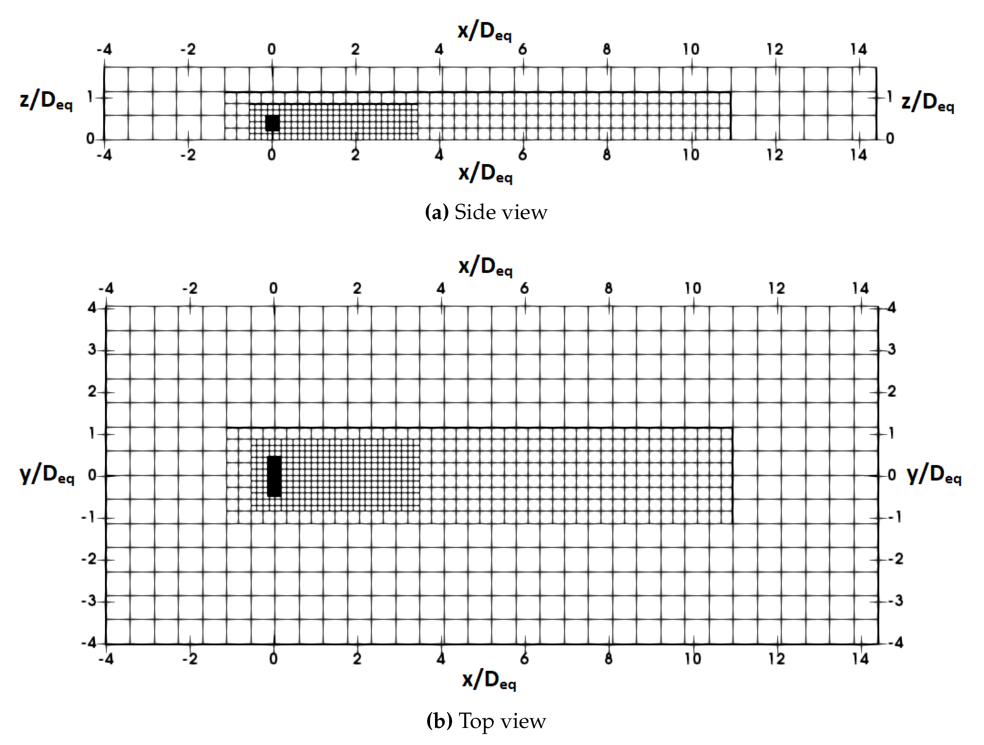
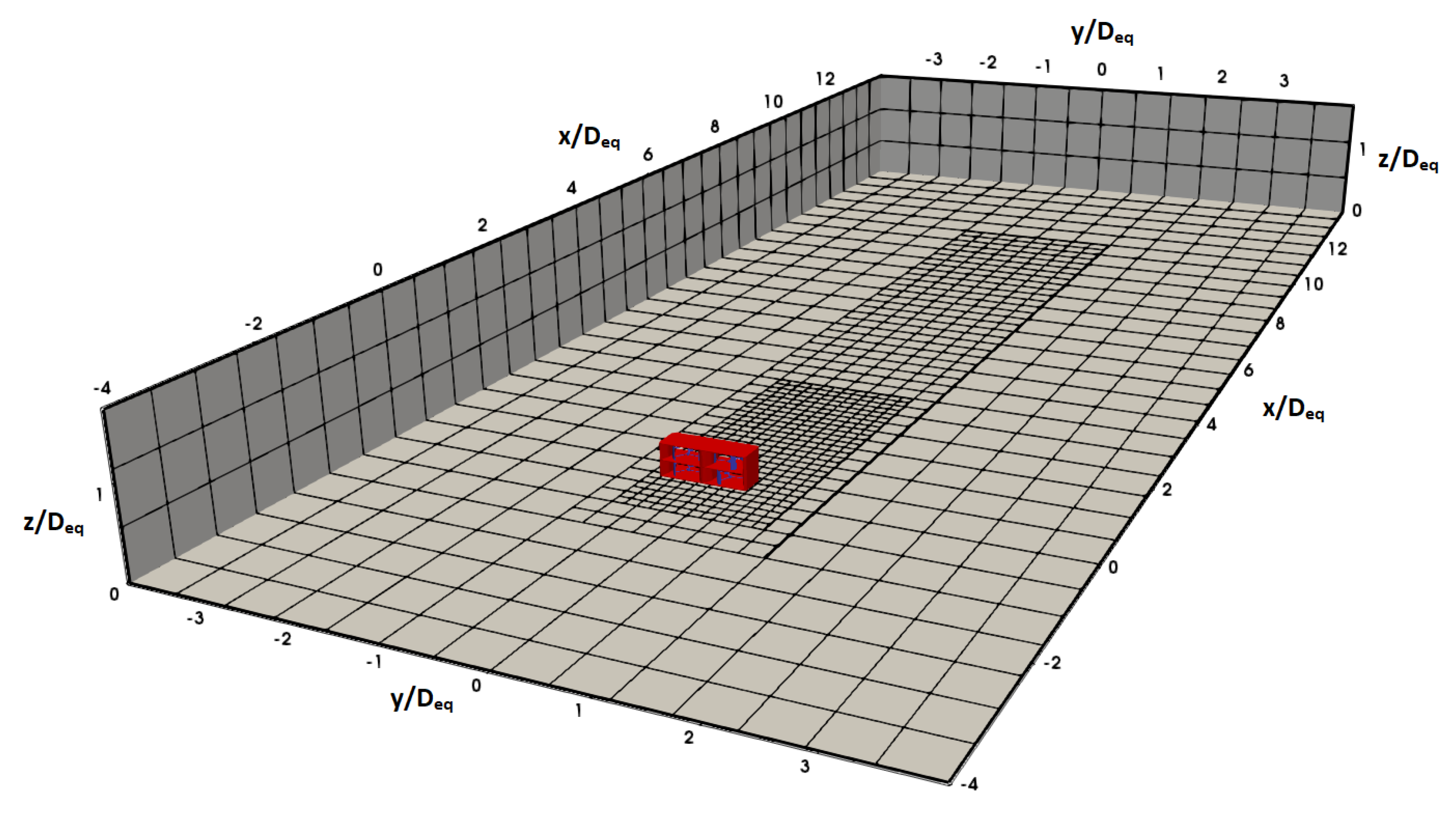
The depth was chosen close to the depth of the Alderney race tidal site [34]: z = 43.12 m. The domain is 460 m long and 200 m wide. The turbine is located 4 D e q downstream of the inlet. The numerical domain is divided into three sub-domains. The finest domain, where the turbine is located, goes up to 3.2 D e q downstream of the turbine. The intermediate domain goes from 3.2 D e q up to 10.5 D e q and the coarsest domain is for the remaining domain. Figure 15 is a cross-sectional view of the mesh and Figure 16 is a three-dimensional view of the computational domain. The finest mesh was chosen according to Section 2.3: Δ x = D / 30 = 0.257 m. There are 12.6 × 10 6 LBM nodes in the mesh and it takes 48.5 h . C P U to compute a single revolution.

3. Results

This section gives the results of the simulations of the turbine presented in Section 2.4. It is divided into two subsections. Section 3.1 is about the influence of inflow conditions over averaged wake quantities. Section 3.2 shows how inflow turbulence influences the shape of the wake.

3.1. Wake Recovery

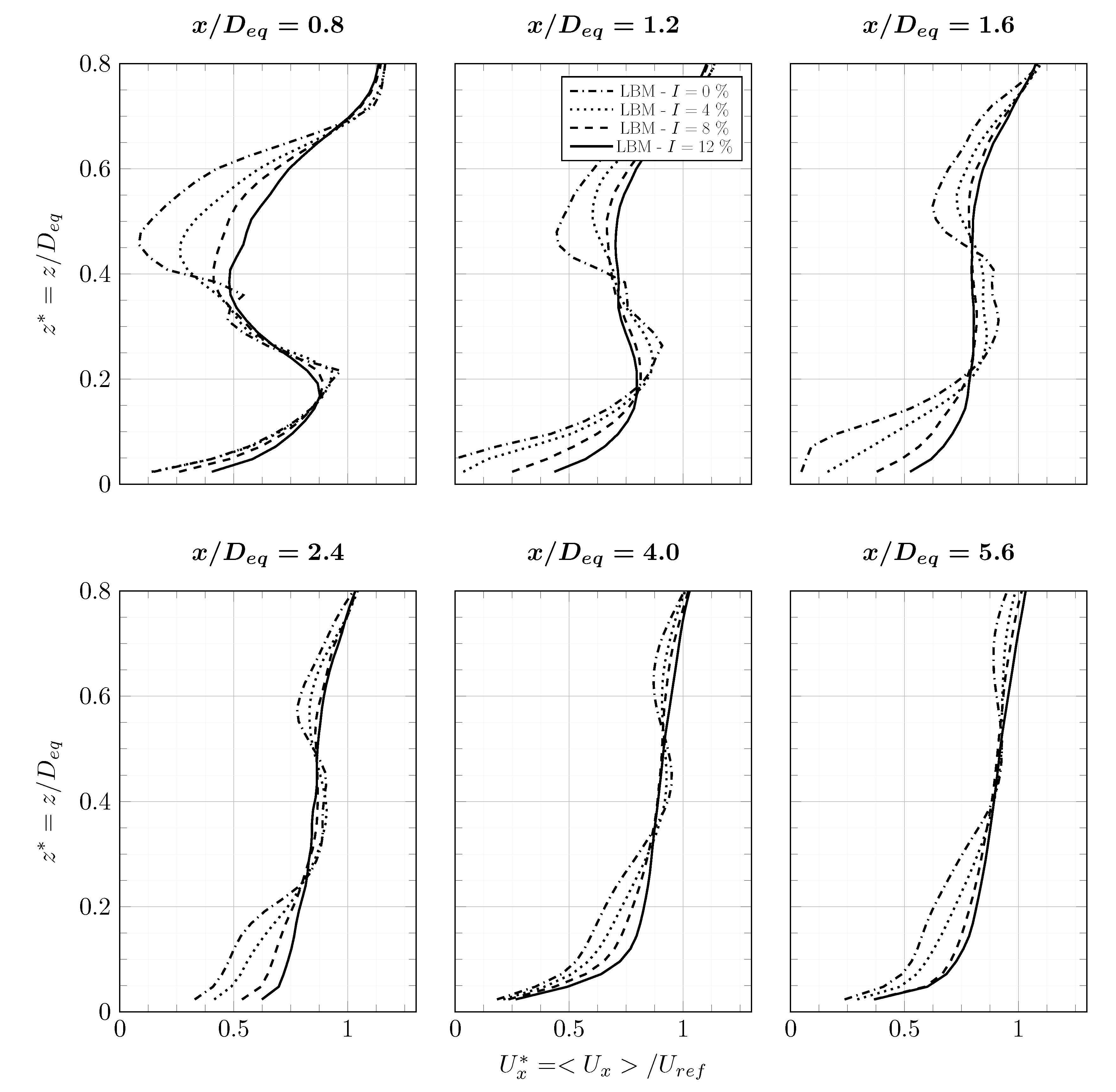
Averages were computed over 60 rotations, after a convergence of 40 rotations. The results were made dimensionless for confidentiality reasons. The average axial velocity < U x > was divided by U r e f . Figure 17 shows the horizontal average axial velocity profiles in the wake of the turbine. Profiles from the bottom rotors and from the top rotors are different, independently of the turbulence rate. The asymmetry according to the y direction is stronger for the bottom profiles than for the top profiles. Because of the upstream velocity profile, the fluid axial velocity at the bottom rotors height is lower than the velocity at the top rotors height. Thus, the tip-speed ratio is higher for the bottom rotors. The asymmetry is counter-intuitive since it should weaken as the tip-speed ratio increases. Differences between the bottom and top profiles tend to be reduced by the ambient turbulence. The higher the turbulent rate is, the lower the asymmetry is. The asymmetry diminishes significantly after 1.6 D e q and even disappears for the higher turbulence rate. The same can be observed on the vertical axial velocity profiles, as visible in Figure 18.
In the close wake, the velocity deficit is greatly influenced by the ambient turbulence. In the far wake, the upstream turbulence intensity seems to have little influence over the horizontal average axial velocity profiles. The turbine footprint is still present 5.6 D e q downstream of the turbine and the maximum velocity deficit is lower than 20 % . However, on the vertical axial velocity profiles, the turbulence seems to affect the velocity deficit in the far wake. The higher the upstream turbulence is, the lower the velocity deficit is.
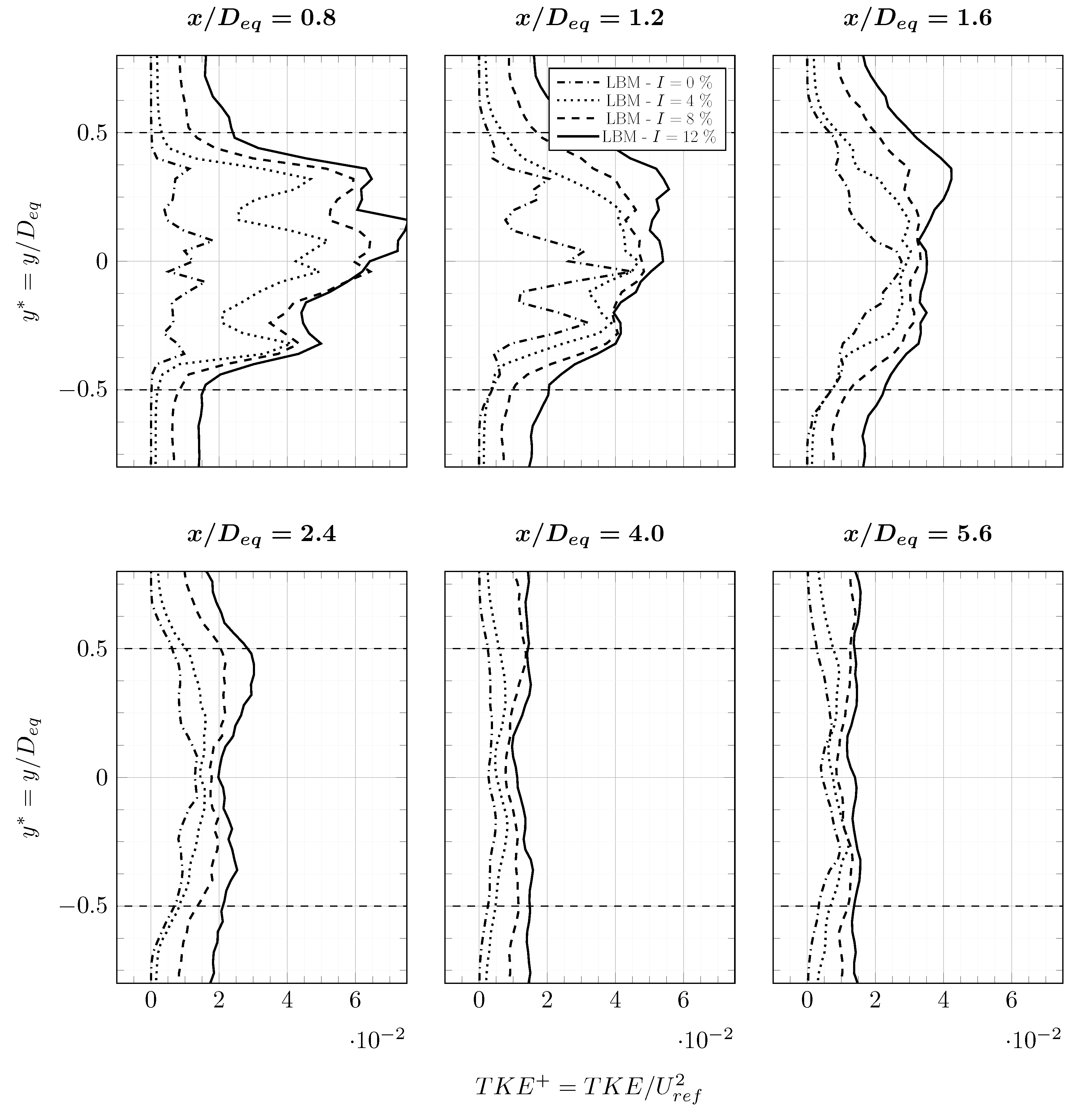
Figure 19 shows the average TKE profiles in the wake of the turbine. In the close wake, 0.8 D e q downstream of the turbine, four peaks can be observed on the I = 0 % and I = 4 % profiles. The two peaks from the positive y side come from the positive y rotors and the two negative y peaks come from the negative y rotors. On the I = 8 % and I = 12 % turbulence intensity profiles, only three peaks are visible: two peripheral peaks coming from the negative y rotors and positive y rotors and one big central peak. This highlight the influence of ambient turbulence over the merging of the wake of the positive y rotors and the negative y rotors. The T K E levels are greatly influenced by the upstream turbulence. A higher upstream turbulence increases the T K E in the wake of the turbine. After 4.0 D e q downstream of the turbine, the T K E levels in the wake are close to the T K E of the ambient flow. However, 5.6 D e q downstream of the turbine, the footprint is still visible for the I = 0 % profile and the T K E is not zero.
Profiles of average wake quantities have been described. The upstream turbulence influence have been highlighted. However, a more comprehensive approach is needed to better understand the influence of ambient turbulence over the wake of the turbine. Such approach is carried out in the next section.

3.2. Wake Structures

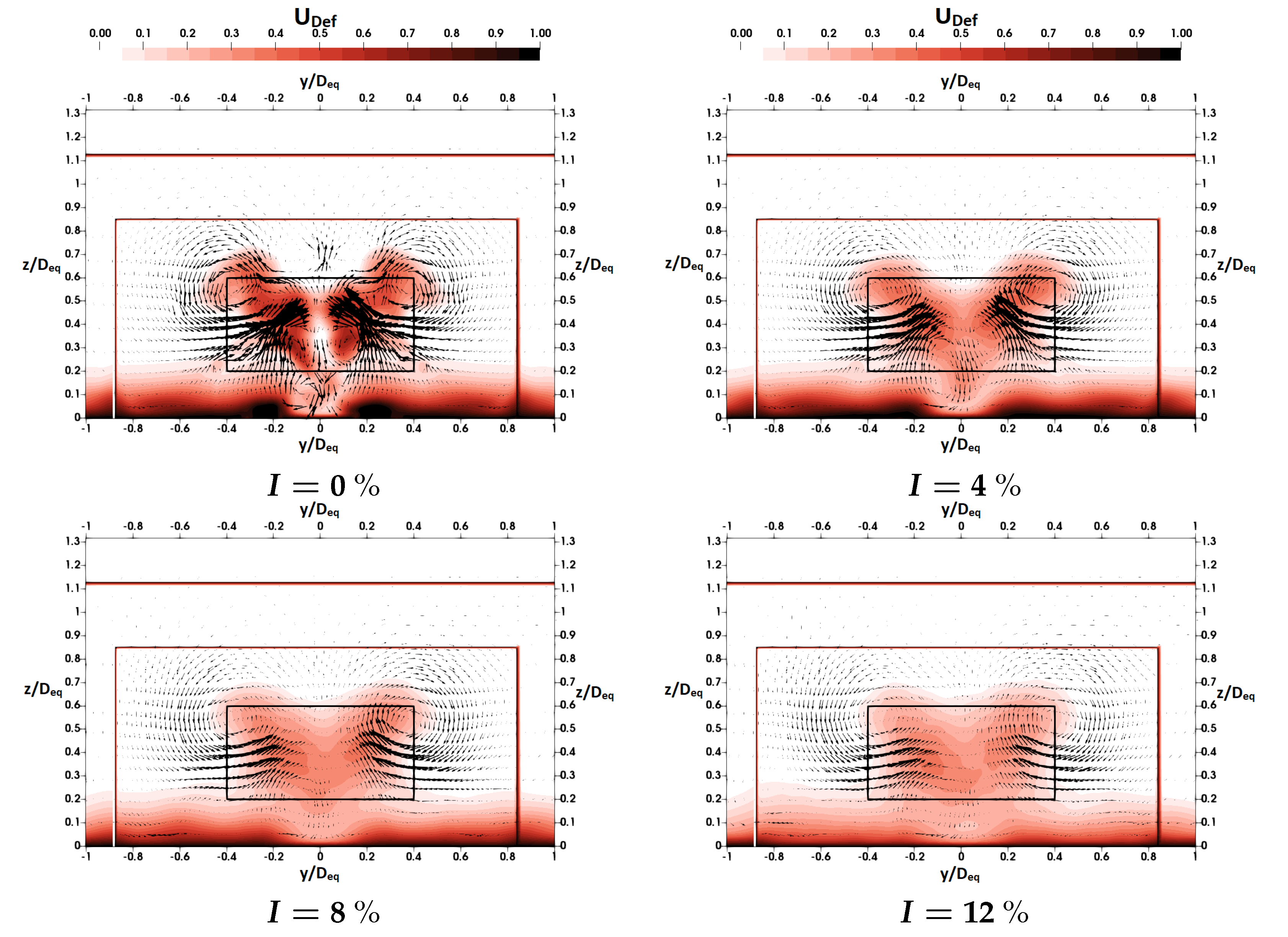
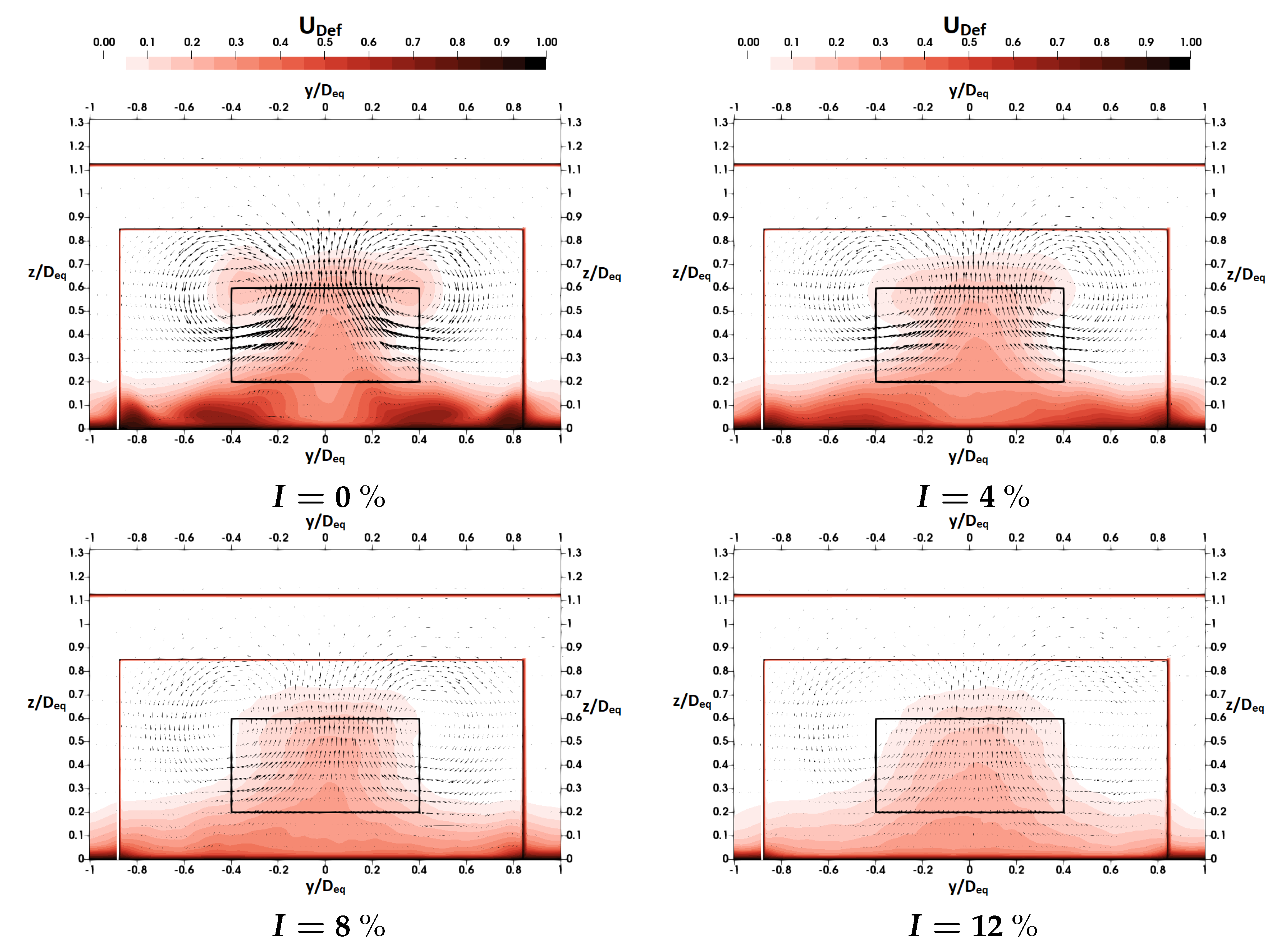
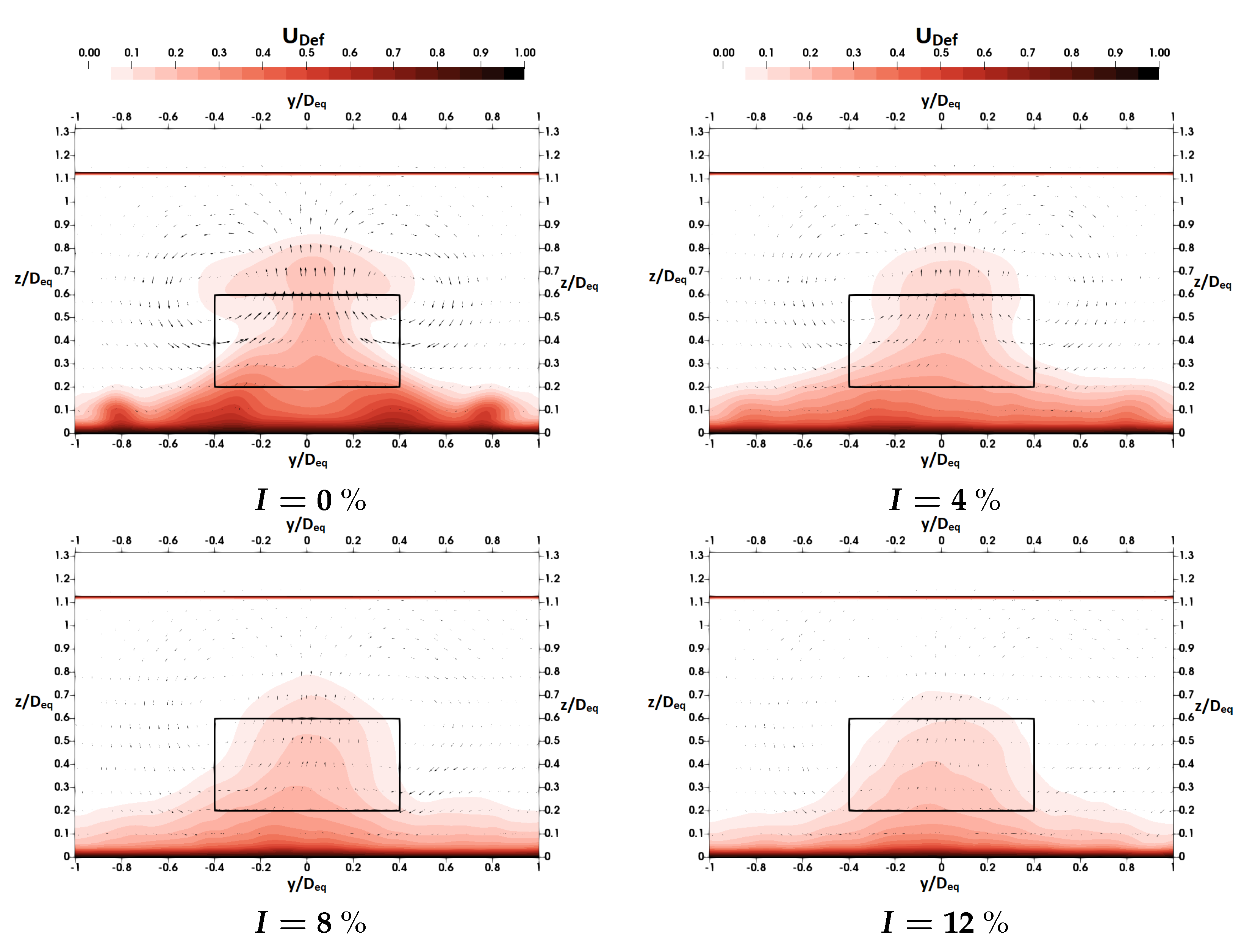
Contours of the velocity deficit in the wake of the turbine are visible 1.2 D e q downstream of the turbine in Figure 20, 3.2 D e q downstream in Figure 21 and 5.2 D e q downstream in Figure 22. Velocity vectors are also projected onto the extracted planes. The influence of ambient turbulence on the shape of the wake is visible at each downstream distance.
In the close wake, 1.2 D e q downstream of the turbine, two distinct wakes are observed on the I = 0 % figure while a single wake is observed on the other profiles. This confirms the influence of turbulence over wakes merging, a phenomenon already highlighted in Section 3.1. Two vortices can be observed at the location of the top corners of the turbine. In Figure 20, those vortices are observed independently of the turbulence rate. However, their intensity seems to be diminished by the ambient turbulence. They appear to be giving the wake a T shape.
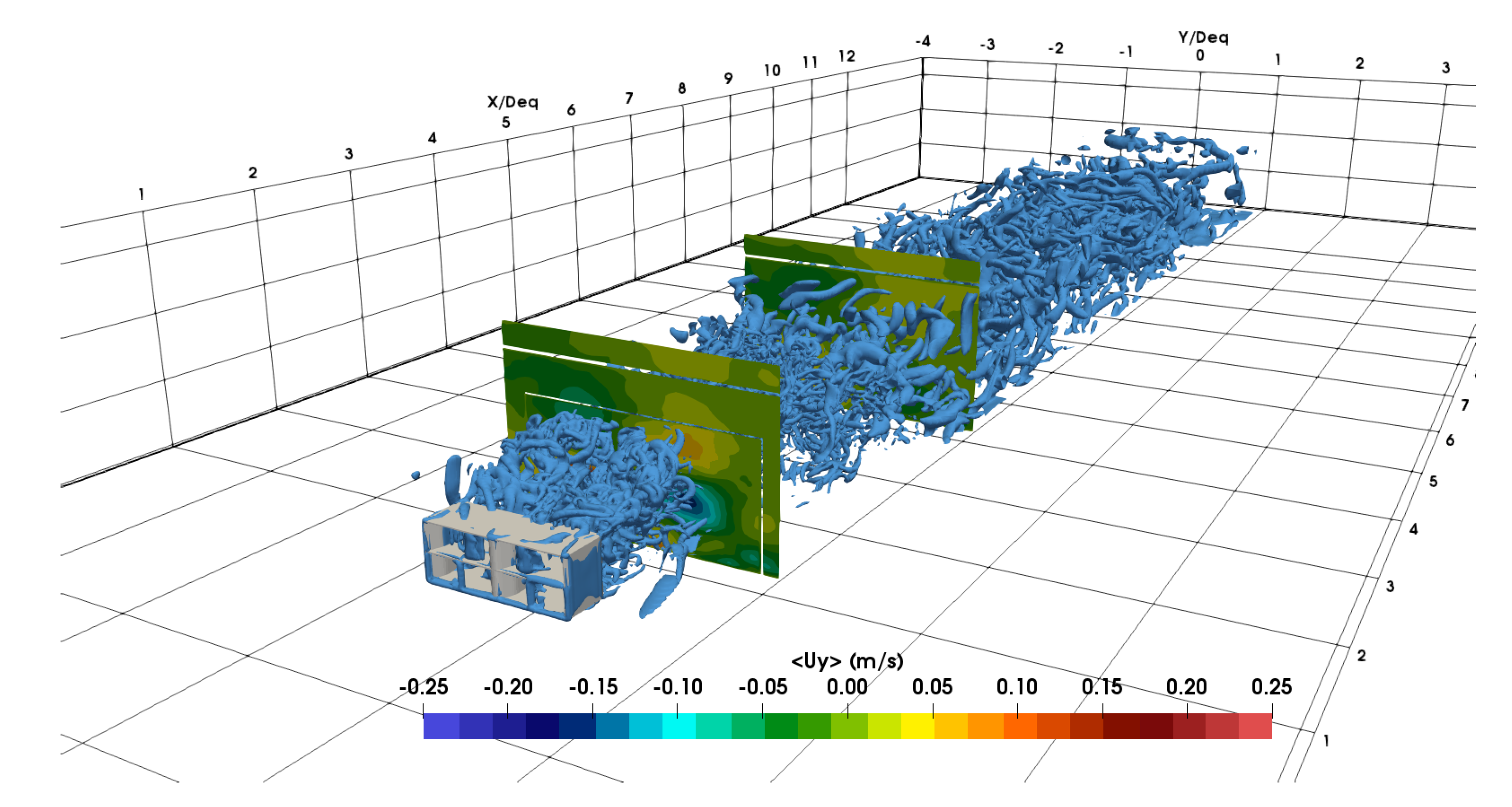
Figure 23 and Figure 24 show instantaneous iso-contours of the L a m b d a 2 criterion in the wake of the turbine for, respectively, I = 0 % and I = 12 % . Planes of the average < U y > velocity are also represented. In both cases, the vortices are visible on the < U y > planes at x / D e q = 1.2 . At x / D e q = 4.2 , the vortices are visible for I = 0 % but much less obvious for I = 12 % . On the instantaneous iso-contours, those vortices are visible as sets of smaller vortices. For I = 0 % , two sets are clearly observable up to x / D e q = 4.2 . For I = 12 % , the two sets are only observable up to x / D e q = 1.2 . The ambient turbulence seems to affect the coherence of the vortices sets. This was seen with the velocity contours and vectors.
At the moment, it is not possible to know whether they are generated by the stator or by the rotor. Further in the wake, the ambient turbulence affects these vortices and causes them to lose their consistency. The shape of the wake is thus influenced and the T shape is smoothed into a square shape. In Figure 22, 5.2 D e q downstream of the turbine, the T shape is observable only on the I = 0 % figure.
As shown in Section 3.1, a strong vertical asymmetry was observed in the close wake. It is possible that this asymmetry is caused by these two vortices. Indeed, at the location of the bottom rotors, the radial velocity is directed toward the turbine center. This phenomenon crushes the wake of the bottom rotors toward the center of the turbine. Since the vortices are weaker for high turbulence rates, the asymmetry is greatly reduced. This is observed in Figure 17.

4. Conclusions

The implementation of an ALM in a LBM solver was realized. The ALM-LBM-LES approach was validated with the experimental case of Rolin and Porté-Agel [27]. A mesh sensitivity study was performed and the mesh Δ x = D / 30 was found to have the highest accuracy. Some discrepancies with the experiment were observed and are most likely due to the low mesh resolution in the viscous sublayer. It is to be noted that there is no tip-loss correction in the ALM-LBM-LES model. Yu et al. [35] showed that adding a tip-loss correction when modeling a horizontal axis wind turbine can reduce the error of the predicted power. It could be an interesting addition to the ALM-LBM-LES model. Nevertheless, the T K E and velocity deficit are relatively well predicted. The shape of the wake is also correctly computed and the two contra-rotating vortices pairs are observed in the close wake, 2.0 D downstream of the turbine.
The ALM-LBM-LES computational cost is a lot lower than LBM-LES blade-resolved approaches. A LBM-LES blade-resolved study of a horizontal axis tidal turbine model was performed by Grondeau et al. [36]. The computational time required to compute a single revolution of the turbine is 450 h.CPU, whereas it is 14 h.CPU for the tidal turbine model simulated here. The same horizontal axis tidal turbine model was studied by Elie et al. [37] with an actuator-disc LES approach. Their code uses an explicit weakly-compressible Navier–Stokes solver. For a mesh size of Δ x = D / 30 , it takes 7.2 h.CPU to compute a revolution of the turbine. It is half the time needed here. However, they only meshed the turbine area with a mesh size of Δ x = D / 30 , thus the number of elements is 7.6 × 10 5 compared to 5.2 × 10 6 here where the wake is also refined at Δ x = D / 30 .
The validated mesh configuration and ALM-LBM-LES model were then used to compute the wake of a real-size tidal turbine. The influence of the turbulence over the wake was assessed. It was observed that the close wake is strongly modified by the upstream turbulence. The influence of ambient turbulence on the far wake is weaker but can still be observed on velocity contours. The presence of two vortices at the top corner of the turbine was highlighted. It was showed that they may have an influence on the vertical asymmetry of the wake. Their intensity and consistency is weakened by the ambient turbulence.
The influence of ambient turbulence on the far wake is limited. Even if the top-corner vortices lose their intensity, they are still observable with I = 12 % , 140.0 m downstream of the turbine. Given the way they affect the shape of the wake, it is possible that they contribute to maintaining the velocity deficit between them. It would then be interesting to use the same numerical configuration to investigate the behavior of the turbine with other turbine configurations, for example with an opposite direction of rotation and without the stator.
After 2.0 D e q , the velocity deficit is relatively low. From the horizontal profiles of the average axial velocity, it is estimated to be around 10 % at x / D e q = 2.4 for I = 12 % . Since it has been shown that the ALM-LBM-LES gives relatively good wake prediction in the close wake, it would be interesting to study a farm with longitudinal spacing starting from [ 2.0 , 2.5 ] D e q . Indeed, one way to optimize tidal farms is to find the smallest distance possible between turbines. A four-turbine farm modeled with the ALM-LBM-LES is estimated to use around [ 200 , 300 ] h.CPU for each revolution of the turbines. Considering the computational resources we have, this would allow us to model several farm configurations.

Author Contributions

Software, M.G., P.M. and E.P.; validation, M.G.; writing–original draft preparation, M.G.; writing–review and editing, M.G., S.G. and E.P.; supervision, S.G.; project administration, S.G.; funding acquisition, S.G.

Funding

This research was funded by Agence de l’Environnement et de la Maîtrise de l’Energie grant number 1682C0085 and Conseil Régional de Normandie grant number 17E01557.

Acknowledgments

This work was funded by l’Agence de l’Environnement et de la Maîtrise de l’Energie (ADEME) [38] in the frame of the OCEANQUEST project and the Région Normandie in the frame of the project SEMARIN. Computational resources were provided by the Centre Régional Informatique et d’Applications Numériques de Normandie (CRIANN) [32] and by the Manche county council. The authors would like to thank Hydroquest [39] for the data provided concerning the Hydroquest/CMN tidal turbine. The authors would like to thank the Palabos project [15], without whom this work would not exist. The authors would also like to thank the ALGLIB project [40] for the open-source interpolation algorithm.

Conflicts of Interest

The authors declare no conflict of interest.

Abbreviations

The following abbreviations are used in this manuscript:
ALMActuator Line Model
CFDComputational Fluid Dynamics
DFSEMDivergence Free Synthetic Eddy Method
LBMLattice Boltzmann Method
LESLarge Eddy Simulation
SEMSynthetic Eddy Method
TKETurbulent Kinetic Energy

References

  1. Multon, B. Energies Marines Renouvelables; Hermes Science: Paris, France, 2011. [Google Scholar]
  2. Clark, T. Turbulence in Marine Environments (TiME): A framework for understanding turbulence and its effects on tidal devices. In Proceedings of the 11th European Wave and Tidal Energy Conference, Nantes, France, 6–11 September 2015. [Google Scholar]
  3. Milne, I.A.; Sharma, R.N.; Flay, R.G.J.; Bickerton, S. Characteristics of the turbulence in the flow at a tidal stream power site. R. Soc. 2013, 371, 196. [Google Scholar] [CrossRef] [PubMed]
  4. Hay, A. Turbulence and Bottom Stress in Grand Passage and Minas Passage; Technical Report; Department of Oceanography, Dalhousie University: Halifax, NS, Canada, 2014. [Google Scholar]
  5. Mycek, P.; Gaurier, B.; Germain, G.; Pinon, G.; Rivaolen, E. Experimental study of the turbulence intensity effects on marine current turbines behaviour. Part I: One single turbine. Renew. Energy 2014, 66, 729–746. [Google Scholar] [CrossRef] [Green Version]
  6. Ouro, P.; Runge, S.; Luo, Q.; Stoesser, T. Three-dimensionality of the wake recovery behind a vertical axis turbine. Renew. Energy 2019, 133, 1066–1077. [Google Scholar] [CrossRef]
  7. Hochman, T.; Martinelli, L.; Smits, A. The effect of inflow conditions on vertical axis wind turbine wake structure and performance. J. Wind. Eng. Ind. Aerodyn. 2018, 183, 1–18. [Google Scholar] [CrossRef]
  8. Brochier, G.; Fraunié, P.; Béguier, C. Water channel experiments of dynamic stall on Darrieus wind turbine blades. J. Propuls. Power 1986, 2, 445–449. [Google Scholar] [CrossRef]
  9. Ouro, P.; Stoesser, T. An immersed boundary-based large-eddy simulation approach to predict the performance of vertical axis tidal turbines. Comput. Fluids 2017, 152, 74–87. [Google Scholar] [CrossRef] [Green Version]
  10. Ahmed, U.; Apsley, D.D.; Afgan, I.; Stallard, T.; Stansby, P.K. Fluctuating loads on a tidal turbine due to velocity shear and turbulence: Comparison of CFD with fields data. Renew. Energy 2017, 112, 235–246. [Google Scholar] [CrossRef]
  11. Shamsoddin, S.; Porté-Agel, F. Large Eddy Simulation of Vertical Axis Wind Turbine Wakes. Energies 2014, 7, 890–912. [Google Scholar] [CrossRef]
  12. Liu, C.; Hu, C. An actuator line—Immersed boundary method for simulation of multiple tidal turbines. Renew. Energy 2019, 136, 473–490. [Google Scholar] [CrossRef]
  13. Guo, Z.; Shu, C. Lattice Boltzmann Method and Its Application in Engineering; World Scientific: Singapore, 2013. [Google Scholar]
  14. Marié, S.; Ricot, D.; Sagaut, P. Comparison between lattice Boltzmann Method and Navier–Stokes high order schemes for computational aeroacoustics. J. Comput. Phys. 2009, 228, 1056–1070. [Google Scholar] [CrossRef]
  15. Available online: https://palabos.unige.ch/ (accessed on 8 November 2019).
  16. Lagrava, S.; Daniel, W.; Malaspinas, O.; Latt, J.; Chopard, B. Advances in multi-domain lattice Boltzmann grid refinement. J. Comput. Phys. 2012, 231, 4808–4822. [Google Scholar] [CrossRef] [Green Version]
  17. Malaspinas, O. Increasing stability and accuracy of the lattice Boltzmann scheme: Recursivity and regularization. arXiv 2015, arXiv:1505.06900v1. [Google Scholar]
  18. Malaspinas, O.; Sagaut, P. Consistent subgrid scale modelling for lattice Boltzmann methods. J. Fluid Mech. 2012, 700, 514–542. [Google Scholar] [CrossRef]
  19. Skordos, P.A. Initial and boundary conditions for the lattice Boltzmann method. Phys. Rev. E 1993, 48, 4823–4842. [Google Scholar] [CrossRef] [PubMed] [Green Version]
  20. Latt, J.; Chopard, B.; Malaspinas, O.; Deville, M.; Michler, A. Straight velocity boundaries in the lattice Boltzmann method. Phys. Rev. E 2008, 77, 056703. [Google Scholar] [CrossRef] [PubMed]
  21. Polleto, R.; Craft, T.; Revell, A. A new divergence free synthetic eddy method for the reproduction of inlet flow conditions for LES. Flow Turbul. Combust. 2013, 91, 519–539. [Google Scholar] [CrossRef]
  22. Grondeau, M.; Mercier, P.; Guillou, S.; Poirier, J.; Poizot, E.; Mear, Y. Numerical simulation of a tidal turbine model in a turbulent flow with the Lattice Boltzmann Method. In Proceedings of the 12th European Wave and Tidal Energy Conference, Cork, Ireland, 27 August–1 September 2017. [Google Scholar]
  23. Shamsoddin, S.; Porté-Agel, F. A large-eddy simulation of vertical axis wind turbine wakes in the atmospheric boundary layer. Energies 2016, 9, 366. [Google Scholar] [CrossRef]
  24. Sørensen, J.N.; Shen, W.Z. Numerical Modling of Wind Turbine Wakes. J. Fluids Eng. 2002, 124, 393–399. [Google Scholar] [CrossRef]
  25. Bachant, P.; Goude, A.; Wosnik, M. Actuator line modeling of vertical-axis turbines. arXiv 2016, arXiv:1605.01449. [Google Scholar]
  26. Mendoza, V.; Bachant, P.; Wosnik, M.; Goude, A. Validation of an actuator line model coupled to a dynamic stall model for pitching motions characteristic to vertical axis turbine. J. Phys. Conf. Ser. 2016, 753. [Google Scholar] [CrossRef]
  27. Rolin, V.; Porté-Agel, F. Exprimental investigation of vertical-axis wind-turbine wakes in boundary layer flow. Renew. Energy 2018, 118, 1–13. [Google Scholar] [CrossRef]
  28. Kumar, V.; Paraschivoiu, M.; Paraschivoiu, I. Low Reynolds Number Vertical Axis Wind Turbine for Mars. Wind. Eng. 2010, 34, 461–476. [Google Scholar] [CrossRef]
  29. Sheldahl, R.E.; Klimas, P.C. Aerodynamics Characteristics of Seven Symmetrical Airfoil Sections through 180-Degree Angle of Attack for Use in Aerodynamic Analysis of Vertical Axis Wind Turbine; Technical Report; Sandia: Albuquerque, NM, USA, 1981. [Google Scholar]
  30. Jarrin, N.; Prosser, R.; Uribe, J.C.; Benhamadouche, S.; Laurence, D. Reconstruction of turbulent fluctuations for hybrid RANS/LES simulations using a Synthetic-Eddy-Method. Int. J. Heat Fluid Flow 2009, 30, 435–442. [Google Scholar] [CrossRef]
  31. Spalding, D. A single formula for the law of the Wall. J. Appl. Mech. 1961, 28, 455–458. [Google Scholar] [CrossRef]
  32. Available online: https://www.criann.fr/ (accessed on 8 November 2019).
  33. Guo, Z.; Zheng, C.; Shi, B. Non-equilibrium extrapolation method for velocity and pressure boundary conditions in the lattice Boltzmann method. Chin. Phys. 2002, 11, 366–374. [Google Scholar]
  34. Thiébaut, M.; Sentchev, A.; Bailly du Bois, P. Merging velocity measurments and modeling to improve understanding of tidal stream resource in Alderney race. Energy 2019, 178, 460–470. [Google Scholar] [CrossRef]
  35. Yu, Z.; Zheng, X.; Ma, Q. Study on actuator line modeling of two NREL 5-MW wind turbine wakes. Appl. Sci. 2018, 8, 434. [Google Scholar] [CrossRef]
  36. Grondeau, M.; Poirier, J.; Guillou, S.; Mear, Y.; Mercier, P.; Poizot, E. Modelling the wake of a tidal turbine with upstream turbulence: LBM-LES versus Navier-Stokes LES. In Proceedings of the 13th European Wave and Tidal Energy Conference, Napoli, Italy, 1–6 September 2019. [Google Scholar]
  37. Elie, B.; Oger, G.; Guillerm, P.E.; Alessandrini, B. Simulation of horizontal axis tidal turbine wake using a Weakly-Compressible Cartesian Hydrodynamic solver with local mesh refinement. Renew. Energy 2017, 108, 336–354. [Google Scholar] [CrossRef]
  38. Available online: https://www.ademe.fr/ (accessed on 8 November 2019).
  39. Available online: http://www.hydroquest.net/ (accessed on 8 November 2019).
  40. Bochkanov, S. ALGLIB. Available online: https://www.alglib.net/ (accessed on 8 November 2019).
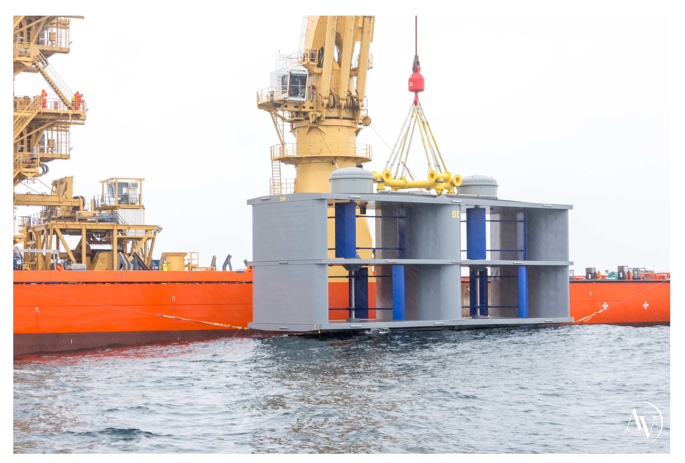
Figure 1. Hydroquest/CMN tidal turbine to be installed at Paimpol-Bréhat test site (France).
Energies 12 04273 g001
Figure 2. Actuator line scheme with: U the upstream velocity, Ω the rotational speed, θ the angular position, C the center of rotation, U ω the tangential velocity, U r e l the relative velocity, α the angle of attack, L the lift force, and D the drag force.
Energies 12 04273 g002
Figure 3. Vertical axis wind turbine tested in Rolin and Porté-Agel [27].
Energies 12 04273 g003
Figure 4. Meshes used for the ALM-LBM mesh sensitivity study. Meshes are represented in cubes of 14 × 14 × 14 nodes. Turbine is represented with the blue cylinder. Plane x y is at turbine mid-height and plane x z is at canal mid-width.
Energies 12 04273 g004
Figure 5. Average axial velocity deficit at different locations in the wake of the turbine. Axis origin is the center of the turbine. Dimensions are scaled by the turbine diameter. The results are from ALM-LBM simulation with Mesh No. 2. U D e f = 1 < U x > / U H / 2 .
Energies 12 04273 g005
Figure 6. Average axial velocity and TKE upstream of the tidal turbine [27]: experimental data and ALM-LBM results for the three meshes. Turbine footprint is drawn in horizontal black dashed-lines.
Energies 12 04273 g006
Figure 7. Average axial velocity deficit y profiles in the wake of the tidal turbine [27] at T S R = 1.1 : experimental data and ALM-LBM results for the three meshes. Turbine footprint is drawn in horizontal black dashed-lines.
Energies 12 04273 g007
Figure 8. Average axial velocity z profiles in the wake of the tidal turbine [27] at T S R = 1.1 : experimental data and ALM-LBM results for the three meshes. Turbine footprint is drawn in horizontal black dashed-lines.
Energies 12 04273 g008
Figure 9. Average axial TKE y profiles in the wake of the tidal turbine [27] at T S R = 1.1 : experimental data and ALM-LBM results for the three meshes. Turbine footprint is drawn in horizontal black dashed-lines.
Energies 12 04273 g009
Figure 10. Average axial TKE z profiles in the wake of the tidal turbine [27] at T S R = 1.1 : experimental data and ALM-LBM results for the three meshes. Turbine footprint is drawn in horizontal black dashed-lines.
Energies 12 04273 g010
Figure 11. Contour of average TKE normalized by the upstream velocity U H / 2 , 2.0 D downstream of the turbine: experimental data from [27] on the left and from the ALM-LBM simulation with Mesh No. 2 on the right. Average velocity vectors are projected onto the plane. Turbine footprint is delimited in black.
Energies 12 04273 g011
Figure 12. Contour of average TKE normalized by the upstream velocity U H / 2 , 6.0 D downstream of the turbine: experimental data from [27] on the left and from the ALM-LBM simulation with Mesh No. 2 on the right. Average velocity vectors are projected onto the plane. Turbine footprint is delimited in black.
Energies 12 04273 g012
Figure 13. Turbine used for the LBM-ALM simulations. Grey parts are modeled in off-lattice and blue parts with forces. The direction of rotation is indicated with red arrows.
Energies 12 04273 g013
Figure 14. Axial velocity profiles obtained from the power law with n = 6.5 and from ADCP measurements in the Alderney Race during ebb [34].
Energies 12 04273 g014
Figure 15. Cross-sectional views of the mesh. The mesh is represented in cubes of 14 × 14 × 14 nodes. Dimensions are scaled by the equivalent diameter D e q = 25.0 m. Axis origin is the center of the turbine. (a): side view at the turbine mid-width. (b): top view at the turbine mid-height.
Energies 12 04273 g015
Figure 16. Illustration of the computational domain. Dimensions are scaled by the equivalent diameter D e q = 25.0 m. The mesh on the domain boundaries is represented in cubes of 14 × 14 × 14 nodes. Stator is in red and rotors are in blue.
Energies 12 04273 g016
Figure 17. Average axial velocity y profiles in the wake of the tidal turbine at T S R = 1.5 . ALM-LBM results for the four turbulence rates. Black curves are extracted at the bottom rotors mid-height. Red curves are extracted at the top rotors mid-height. Turbine footprint is drawn in horizontal black dashed lines. Dimensions are scaled by the equivalent diameter D e q = 25.0 m.
Energies 12 04273 g017
Figure 18. Average axial velocity z profiles in the wake of the tidal turbine at T S R = 1.5 . Vertical profiles aligned with rotors center. Since y profiles are symmetrical, only the profiles from the positive y side rotors are shown. ALM-LBM results for the four turbulence rates. Dimensions are scaled by the equivalent diameter D e q = 25.0 m.
Energies 12 04273 g018
Figure 19. Average T K E + y profiles in the wake of the tidal turbine at T S R = 1.5 . Horizontal profiles extracted at the turbine mid-height. ALM-LBM results for the four turbulence rates. Turbine footprint is drawn in horizontal black dashed lines. Dimensions are scaled by the equivalent diameter D e q = 25.0 m.
Energies 12 04273 g019
Figure 20. Contour of axial velocity deficit, 1.2 D e q downstream of the turbine. Velocity vectors are projected onto the plane. Turbine footprint is delimited in black. ALM-LBM simulations with four turbulence rates. U D e f = 1 < U x > / U r e f .
Energies 12 04273 g020
Figure 21. Contour of axial velocity deficit, 3.2 D e q downstream of the turbine. Velocity vectors are projected onto the plane. Turbine footprint is delimited in black. ALM-LBM simulations with four turbulence rates. U D e f = 1 < U x > / U r e f .
Energies 12 04273 g021
Figure 22. Contour of axial velocity deficit, 5.2 D e q downstream of the turbine. Velocity vectors are projected onto the plane. Turbine footprint is delimited in black. ALM-LBM simulations with four turbulence rates. U D e f = 1 < U x > / U r e f .
Energies 12 04273 g022
Figure 23. Average < U y > velocity planes at x / D e q = 1.2 and x / D e q = 4.2 in the wake of the turbine for an upstream turbulence rate of I = 0 % . Dimensions are scaled by the equivalent diameter D e q = 25.0 m. Vortices are represented with instantaneous iso-contour of the L a m b d a 2 criterion, L a m b d a 2 = 1.0 × 10 5 . x and y axis are centered at the turbine location.
Energies 12 04273 g023
Figure 24. Average < U y > velocity planes at x / D e q = 1.2 and x / D e q = 4.2 in the wake of the turbine for an upstream turbulence rate of I = 12 % . Dimensions are scaled by the equivalent diameter D e q = 25.0 m. Vortices are represented with instantaneous iso-contour of the L a m b d a 2 criterion, L a m b d a 2 = 1.0 × 10 5 . x and y axis are centered at the turbine location.
Energies 12 04273 g024
Table 1. Rotor configuration from Rolin and Porté-Agel [27].
QuantityValueUnit
Number of blades n3~
Rotor Radius R 0.083 m
Blades height H 0.155 m
Chord length c 0.03 m
Solidity S d 0.54 ~
Tip Speed Ratio λ 1.1 ~
Reynolds number (radius) 5.0 × 10 4 ~
Table 2. Configurations for the ALM-LBM mesh sensitivity study. h.CPU is wall-clock-time multiplied by the number of CPU used.
Mesh D / Δ x Δ x  (m) Δ t  (s)Number of Nodesh.CPU per rev.
No. 115 11.16 × 10 3 3.04 × 10 5 1.5 × 10 6 1.6
No. 230 5.58 × 10 3 1.52 × 10 5 5.2 × 10 6 14
No. 350 3.34 × 10 3 0.91 × 10 5 22.5 × 10 6 128
Table 3. Root-mean-square of the error on the U x * and T K E +  z profiles. Error is averaged between z / D = 0.316 and z / D = 1.25 .
Mesh U x * at 4 D TKE + at 4 D U x * at 8 D TKE + at 8 D U x * at 10 D TKE + at 10 D
No. 1 22.0 % 48.3 % 5.3 % 37.6 % 5.2 % 24.4 %
No. 2 11.0 % 18.4 % 5.8 % 14.4 % 6.9 % 16.0 %
No. 3 6.8 % 19.6 % 5.1 % 37.1 % 6.0 % 43.2 %
Table 4. Rotor configuration.
QuantityValueUnit
Number of blades n3~
Rotor Radius R 4.0 m
Blades height H 3.8 m
Tip-Speed Ratio λ 1.5 ~
Reynolds number (radius) 5.9 × 10 6 ~