Fractional-Order Modeling and Parameter Identification for Ultracapacitors with a New Hybrid SOA Method

Abstract

This paper deals with an ultracapacitor (UC) model and its identification procedure. To take UC’s fractional characteristic into account, two constant phase elements (CPEs) are used to construct a model structure according to impedance spectrum analysis. The different behaviors of UC such as capacitance, resistance, and charge distribution dynamics are simulated by the corresponding part in the model. The resistance under different voltages is calculated through the voltage rebound method to explore its non-linear characteristics and create a look-up table. A nonlinear fractional model around an operation voltage is then deduced by applying the resistance table. This time identification is carried by a proposed hybrid optimization algorithm: Nelder-Mead seeker algorithm (NMSA), which embeds the Nelder–Mead Simplex (NMS) method into the seeker optimization algorithm (SOA). Its time behavior has been compared with the linear fractional model for charging and discharging current profiles at different levels.

1. Introduction

Ultracapacitors (UCs) are currently gaining attention rapidly as a new type of energy-storage component with a higher density than ordinary capacitance and longer cycle life than batteries [1,2]. However, its energy storage principle determines its capacity cannot temporarily surpass the battery [3]. Thence, it is always associated with batteries in the energy storage unit when it supplies energy to electric vehicles (EV) or hybrid electric vehicles (HEV). UC can meet vehicle startup and acceleration requirements due to its high power rate. Thanks to the short charging time of UC, the braking energy can be absorbed efficiently during decelerating. With a reasonable power distribution strategy in-vehicle, the application of UC is a good way to reduce battery load and further to improve the battery’s cycle life.

In the early stage of UC modeling, the internal properties of UC are analyzed in many electrochemical models. In their model, Gouy and Chapman adopted the principle that ion distribution of the double-layer’s outer element conformed to the laws of Bolzmann [4]. The mathematical model proposed in [5] described the effect of pore size on UC performance. On the contrary, the machine learning model describes the relationships between inputs and outputs without considering the internal structure. The subject [6,7,8] utilized ANN technology to predict the performance of carbon materials in supercapacitors. Among all the modeling approaches, the equivalent circuit model is the most commonly used. Through studying the slow charging behavior of UC, R.L. Spyker and R.M. Nelms used a classical equivalent circuit composed of capacitance in parallel with resistance and an equivalent series resistance [9]. To take into account the fast dynamics, a model consisting of three RC branches is proposed that reflected the internal charge distribution process within a specific voltage range [10]. Because of the widespread use of activated carbon with high surface area, some groups adopted the transmission line model (TLM) to simulate the frequency response of UC and discussed the contribution of the parameters to the impedance spectrum [11]. The complex determination of different elements and large numbers of parameters leads to inconvenience.

To simplify the complexity of the model, the fractional-order model has been employed. A simple UC model composed of a series resistor and a CPE is used to model the impedance in the frequency range in [12]. The capacitance-voltage dependence is taken into account in [13] by implanting a voltage-dependent capacitance in one of the three branches and a fitting formula with an undetermined coefficient is used. N. Bertrand et al. [14] used a set of linear systems to deduce a global nonlinear model.

In a process of model identification, there are traditional methods such as the least square methods, the gradient-based methods, and the maximum likelihood methods. They can be suitable for nonlinear systems after some efforts made by [15]. However, the recognition process of all the above methods needs to derive the objective function, which is difficult to implement in fractional-order systems. The derivative-free algorithms, such as the simplex search method [16] and Nelder–Mead simplex (NMS) algorithm, [17] are successfully applied to the parameter tuning. The limitations of these techniques are the natural local concern and the sensitivity to the initial solution of the algorithm. Fractional order system identification problems have been carried out using global heuristic techniques such as particle swarm optimization (PSO) [18], genetic algorithm (GA) [19], and artificial bee colony algorithm (ABC) [20]. Compared to the local search algorithm, they have a global performance nature and a greater possibility to converge to the global optimal point. Nevertheless, they often oscillate in the vicinity of the optimal point or miss the optimal area due to strong randomness.

The seeker optimization algorithm (SOA) is also a heuristic algorithm, which was invented by Dai [21]. It explores the experience of human search behavior through the analysis of the human random search process. By exchanging experience, seekers determine their direction and step size, then update their location, and, finally, find the optimal point. Since it is proposed, it has been used by researchers in different engineering applications like system modeling and optimal control [22,23]. To overcome the individual limits of SOA, a hybridization of SOA and NM algorithm is used in this paper, which simultaneously retains the benefits of both techniques while discarding their drawbacks.

The proposed modeling approach leads to a model that has the following characteristics:

⬤

The model structure is connected to UC dynamic characteristics;

⬤

The using of fractional order reduces the number of parameters;

⬤

The resistance voltage dependence has been taken into account;

⬤

The hybrid optimization algorithm improves recognition accuracy.

2. Fractional-Order Calculus

Fractional-order calculus (FOC) generalizes the integrals and derivatives from integer-order to arbitrary real order. This theory goes back to a note written by Leibniz, in which the meaning of the half-derivative of the function x was discussed. Some approaches to generalizations of the notion of calculus can be found in [24]. A great deal of work has been done to propose the models of linear time-invariant system and nonlinear system for analyzing the stability, time, frequency domain response, and other properties of the fractional-order model [25,26]. FOC provides an excellent instrument for the description of stochastic memory phenomena such as electrochemical phenomena, chaos, and viscoelasticity. Consider a function $y=f\left(t\right)$, which is integrable and has at least $m\left(mϵN\right)$ continuous derivatives. The universal expression of integer-order derivatives and integrals is as follows:

$${}_a{}^{}D{}_t^{p}f\left(t\right)=\underset{h\to 0}{lim}{h}^{-p}{\sum }_{r=0}^n{(-1)}^r\left(\begin{array}{c}p\\ r\end{array}\right)f\left(t-rh\right),$$

(1)

$$\left(\begin{array}{c}p\\ r\end{array}\right)=\frac{p\left(p-1\right)\left(p-2\right)\cdots \left(p-r+1\right)}{r!}$$

(2)

$\left(\begin{array}{c}p\\ r\end{array}\right)$ is the usual notation for the binomial coefficient, $n=\left[\left(t-a\right)/h\right]$. For $p=m\left(m>0\right)$, ${}_a{}^{}D{}_t^p=\frac{d^{m}t}{d{t}^m}$ represents the derivative of order $m$. On the contrary, ${}_a{}^{}D{}_t^p$ denotes $m$ fold integral if $p=-m\left(m>0\right)$. The unification of integer-order derivatives and integrals is the basis for allowing p in (1) to be an arbitrary real number or even a complex number. In this section, three main definitions of fractional order integrals and derivatives are briefly introduced.

⬤

Grünwald–Letnikov Definition:

$${}_a{}^{}D{}_t^{\alpha }f(t)=\underset{h\to 0}{lim}{h}^{-\alpha }{\displaystyle \sum }_{r=0}^n{\left(-1\right)}^r\left(\begin{array}{c}\alpha \\ r\end{array}\right)f\left(t-rh\right),\left(m-1<\alpha <m\right)$$

(3)

$$\left(\begin{array}{c}\alpha \\ r\end{array}\right)=\frac{1}{\left(\alpha +1\right)B\left(\alpha -r+1,r+1\right)}$$

(4)

⬤

Riemann–Liouville Definition:

$${}_a{}^{}D{}_t^{\alpha }f\left(t\right)=\frac{1}{\Gamma \left(m-\alpha \right)}\frac{d^m}{dt}{\int }_a^t{\left(t-\tau \right)}^{m-\alpha -1}f\left(\tau \right)d\tau ,\left(m-1<\alpha <m\right)$$

(5)

⬤

Caputo definition:

$${}_a{}^{}D{}_t^{\alpha }f\left(t\right)=\frac{1}{\Gamma \left(m-\alpha \right)}{\int }_a^t{\left(t-\tau \right)}^{m-\alpha -1}{f}^{\left(m\right)}\left(\tau \right)d\tau ,\left(m-1<\alpha <m\right)$$

(6)

Grünwald–Letnikov generalizes integer-order calculus directly and requires that $f\left(t\right)$ can be differentiated $m=\left[\alpha \right]+1$ times ($\alpha \in R$). However, a limit operation is not convenient. Rieman–Liouville provides an excellent opportunity to weaken the requirement for the differentiability of $f\left(t\right)$ through m-α-1 times integral before m-order derivative. Another definition was proposed by M.Caputo that exchanges the sequence of derivative and integral. The main advantage of the Caputo approach is permitting the initial conditions for fractional differential equations to take on the same form as for integer-order differential equations, which makes them easy to interpret. Another difference between Caputo’s definition and the other two definitions can be shown in the derivative of a constant C. The Caputo derivative of a constant is 0, whereas the other two bring a nonzero value as Equation (7), so the Caputo definition is used in this paper.

$${}_a{}^{}D{}_t^{\alpha }C=\frac{C{t}^{-\alpha }}{\Gamma \left(1-\alpha \right)}$$

(7)

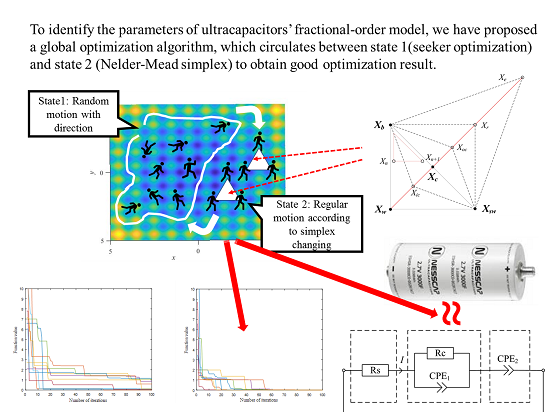
3. A New Hybrid Algorithm: NMSA

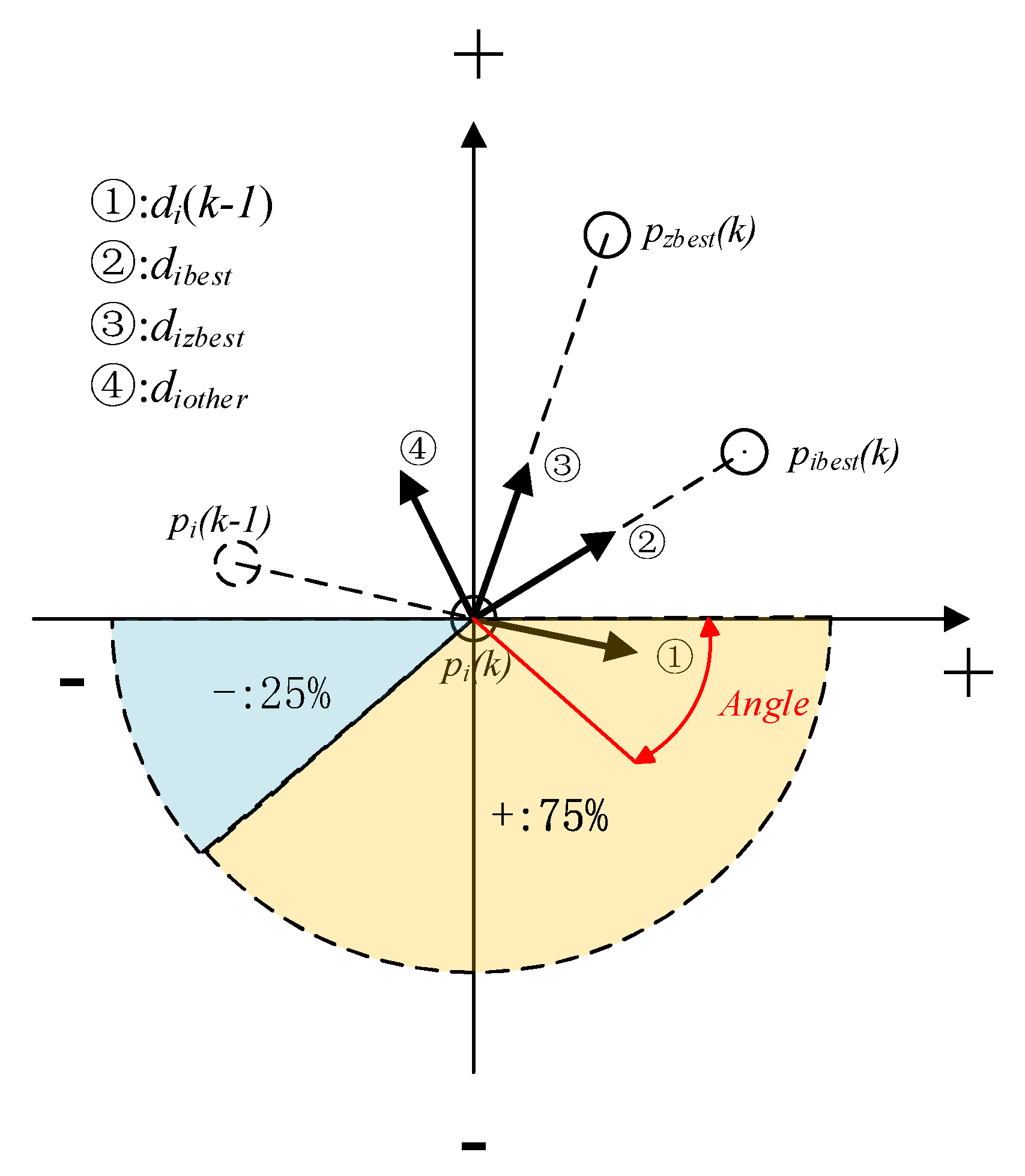
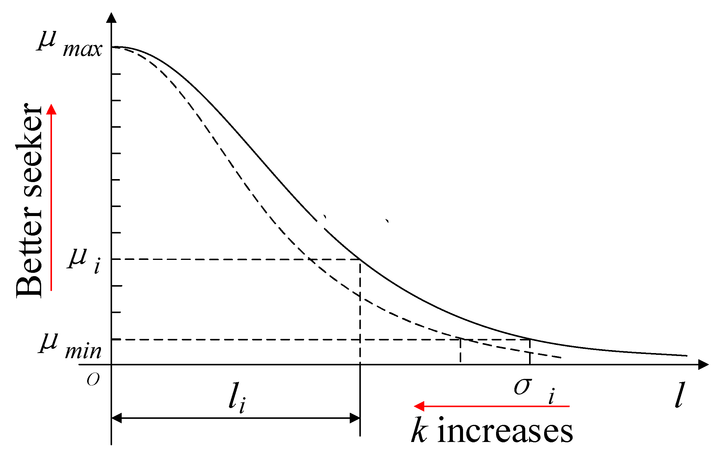
3.1. Seeker Optimization Algorithm (SOA)

SOA is a new swarm intelligence optimization algorithm, which has better optimization quality and robustness than GA and PSO [21]. It resolves optimization problems by means of map search. n seekers search for the lowest position on the D-dimension map if there are D optimized variables. The lowest position stands for the set of optimal parameters and the height of a point is calculated by the objective function. Their journey lasts for g days, to begin with, they are sent to the initial position randomly on the first day. On each of the following days, they need to record the lowest place they have ever been and the corresponding altitude. Meanwhile, they share their locations and altitudes with the information network, which can be read by everyone and the best location of the past few days can be selected. Afterward, according to several reference locations, each seeker determines the direction and distance to go tomorrow, following a certain rule, and start their search the next day. They move, communicate, and make plans at the end of the day journey until their whole journey is finished and a position closest to the bottom is found.

On kth day, ith seeker $p_i\left(k\right)$ has a tendency to move towards the personal best position $p_{ibest}\left(k\right)$ and the best position of population $p_{zbest}\left(k\right)$. Meanwhile, he tends to inherit the moving direction $d_i\left(k-1\right)$ of the yesterday if $f\left(p_i\left(k\right)\right)<f\left(p_i\left(k-1\right)\right)$ and to reverse it if not. Another reference direction might also exist, which is represented by $d_{iother}\left(k\right)$. Those reference directions are marked in Figure 1. Using horizontal as an example, after the number of reference directions toward the positive direction and those toward the negative direction are counted, respectively, draw the probability distribution semicircle. Then ith seeker determines his moving direction $d_i\left(k\right)$ by generating a random angle. If the angle is as shown in Figure 1, the ith seeker moves positively in horizontal.

The search step length $l_i\left(k\right)$ is calculated by Gaussian membership function in Equation (8). ${\mu }_i$ is a decreasing function of ith seeker’s fitness ranking I_i. I_i means that $f\left(p_i\left(k\right)\right)$ is the $I_i$th lowest in all $f\left(p\left(k\right)\right)$. ${\sigma }_i$ is negatively correlated with k. ${\mu }_i$ allows the seeker near the optimal point to search for more details and ${\sigma }_i$ makes seekers search more carefully at the later stage of the search. Figure 2 is an intuitive expression for determining the step length. ‘→’ represents the tendency to lessen step length.

$$\mu \left(l_i\right)=e^{-\frac{l_i^2}{2{\sigma }_i^2}}$$

(8)

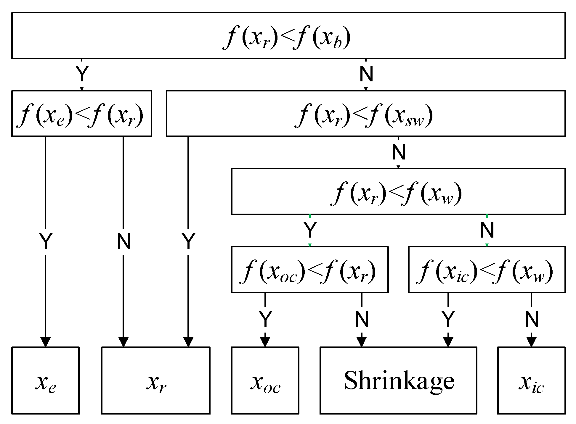
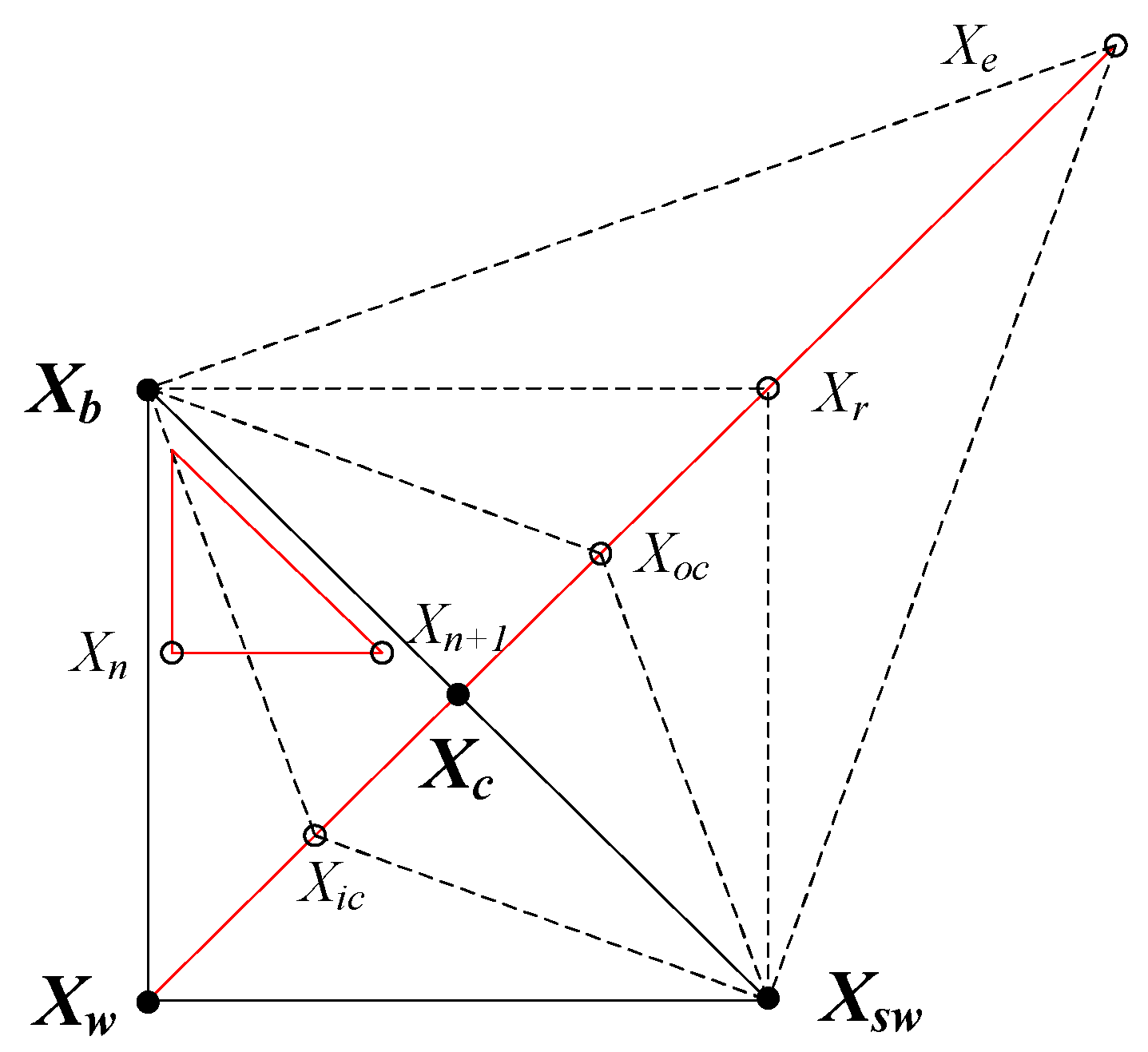
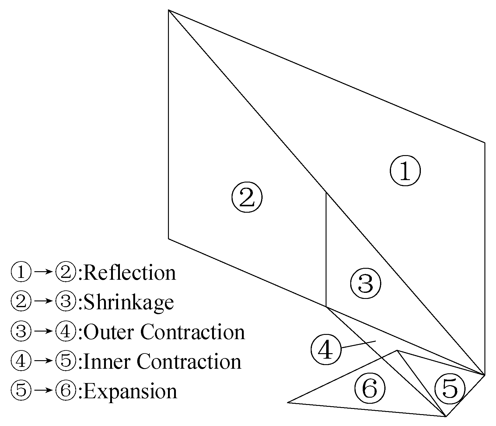
3.2. Nelder–Mead Simplex Algorithm

As a derivative-free method, the NM algorithm is used to construct a simplex to solve unconstrained minimization problems. To minimize a mathematical function $f$ that has $n$ real parameters, the simplex is designed with $n+1$ vertexes and to replace the worst vertex with a better one each iteration via reflection, expansion, contraction, or reduction.

After the initial simplex is determined, the function $f$ is evaluated at each of the vertices, which are later renamed according to its value and then comes the relationship in Equation (9). The basis points and the candidate points that will be used later are listed in

Table 1. Basis points and the candidate points of Nelder–Mead (NM).

Basis		Candidate
Best vertex	$X_b=X_1$	Reflection point	$X_r=X_c+\alpha \left(X_c-X_w\right)$
Second worst vertex	$X_{sw}=X_n$	Expansion point	$X_e=X_c+\beta \left(X_r-X_c\right)$
Worst vertex	$X_w=X_{n+1}$	Outer contraction point	$X_{oc}=X_c+\gamma \left(X_r-X_c\right)$
Centroid	$X_c=\frac{1}{n}{\displaystyle \sum _{i=1}^n}{X}_i$	Inner contraction point	$X_{ic}=X_c+\gamma \left(X_w-X_c\right)$
		Shrinkage points	$\begin{array}{l}{X}_s\left(i\right)=X_b+\delta \left(X_i-X_b\right)\\ i=2, 3,\dots , n+1\end{array}$

. And they are elected pursuant to the rule shown in Figure 3. The NM algorithm is the first step towards finding an effective substitute for $X_w$ along the line segment joining $X_c$ and $X_w$ as seen in Figure 4. If the first step fails, NM no longer explores that line segment but starts to draw closer to $X_b$ by shrinking. Figure 5 shows the evolution of simplex when NM is used to find the optimal point of a 2-dimensional objective function.

$$f\left(X_1\right)\le f\left(X_2\right)\le \cdots \le f\left(X_{n+1}\right)$$

(9)

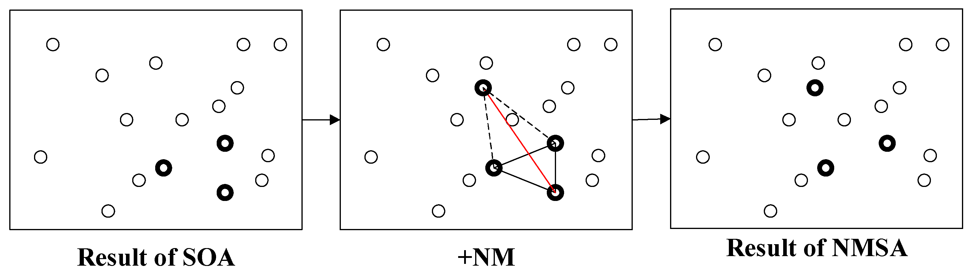
3.3. New Hybrid SOA: NMSA

The random factors in the seeker’s direction and step length bring SOA good global exploration ability. Nevertheless, it is also the randomness that causes its poor local exploration ability. SOA’s later search is always wasted. Besides, when dealing with a multi-extremum problem, SOA may converge to a wrong extreme point because of insufficient exploration to the main extreme point. As a beam search method, the NM simplex method has opposite capability compared with SOA. However, it also produces incorrect outputs due to the quality of the initial simplex. In this paper, a synthetic algorithm of NM and SOA is proposed to make their respective advantages complementary to each other. In every day’s searching, the top $n+1$ seekers of SOA do the NM transformation and iterate once. After that, they begin to share their positions and to make the next day’s plan. A diagram of the proposed method NMSA (The hybrid algorithm based on the seeker algorithm and the Nelder–Mead simplex) is given in Figure 6.

To evaluate the performance of the optimization strategy, a set of artificial test functions has been proposed and used as benchmarks. Typically, they can be classified in the term of modality. If there is only one peak in the function landscape, the function is said to be unimodal (e.g., sphere function, booth function, etc.), which is often used for convergence velocity comparison [27]. On the contrary, the function is a multimodal function (e.g., Rastrigin function, Ackley function, Schwefel function, etc.). It turns out to be an extremely important performance test for global optimization because it creates difficulties in finding a global minimum. In such a landscape, the search process can direct the search away from the true optimal solutions and trapped in one of the local minima.

For our proposed offline global optimization algorithm NMSA, its reliability and precision should be tested. Rastrigin function, one of the multimodel functions, is based on De Jong’s function with the addition of cosine modulation to produce many local minima. In addition, the small fitness differences in the topology increase the complexity of the problem [28]. Therefore, consider the Rastrigin function as the test function of NMSA. The function is given by the following formula and visualized by Figure 7.

$$f\left(x,y\right)=x^2+y^2-10\mathit{cos}\left(2\mathsf{\pi }x\right)-10\mathit{cos}\left(2\mathsf{\pi }y\right)+20$$

(10)

Rastrigin function has several minima. The global one is at (0, 0). This minimum gives a function value $f=0$. The nearest other minima are, respectively, at (0, 1), (0, −1), (1, 0), and (−1, 0), and they all give a value $f=1$. As shown in Figure 8, based on the respective function value obtained by NMSA and SOA after 10 runs, it can be noted that the NMSA algorithm leads successfully to the global minimum compared with the original SOA. With SOA, nearly half of the optimization processes converge to secondary minima and the remainder need at least 90 iterations to converge to the global minimum. NMSA needs less than 60 iterations to get the correct minimum with no wrong judgments in 10 runs. That is because NM offsets the SOA’s weakness in local exploration and improves the directionality in NMSA. In general, NMSA has the following characteristics: (1) Its global and local exploration abilities are well balanced for finding the global minimum; (2) It has combined the ergodicity and directionality effectively for a faster rate of convergence. In

Table 2. Results of SOA and NMSA.

${\left(\mathit{x},\mathit{y}\right)}_{\mathit{s}\mathit{e}\mathit{a}\mathit{r}\mathit{c}\mathit{h}\mathit{e}\mathit{d} \mathit{b}\mathit{y} \mathit{S}\mathit{O}\mathit{A}}$	$\mathit{f}\left(\mathit{x},\mathit{y}\right)$	${\left(\mathit{x},\mathit{y}\right)}_{\mathit{s}\mathit{e}\mathit{a}\mathit{r}\mathit{c}\mathit{h}\mathit{e}\mathit{d} \mathit{b}\mathit{y} \mathit{N}\mathit{M}\mathit{S}\mathit{A}}$	$\mathit{f}\left(\mathit{x},\mathit{y}\right)$
(+8.8432E−3, −1.1794E−2)	+4.3093E−2	(+1.1729E−3, +6.7883E−3)	+9.4136E−3
(−2.0045E−3, −2.9132E−3)	+2.4808E−3	(−4.1521E−3, +3.3201E−5)	+3.4204E−3
(−1.0142E00, −6.2758E−3)	+1.0763E00	(−4.3177E−4, −1.2294E−3)	+3.3684E−4
(+6.6242E−2, −5.0537E−3)	+8.6317E−1	(+2.7027E−3, −7.0799E−3)	+1.1392E−2
(+1.0154E00, −6.6096E−3)	+1.0867E00	(−9.5493E−3, +3.2802E−3)	+2.0220E−2
(+2.1976E−2, −1.4773E−2)	+1.3893E−1	(+2.2814E−3, +6.8896E−4)	+1.1267E−3
(−1.7572E−2, +8.4259E−3)	+7.5280E−2	(−2.1941E−3, −2.5050E−2)	+4.4583E−3
(−9.7707E−1, −2.2125E−2)	+1.1553E00	(−3.0697E−4, +2.6148E−3)	+1.3751E−3
(−2.0418E−2, −5.1174E−2)	+5.9771E−1	(−5.7813E−4, −1.8963E−3)	+7.7976E−4
(+2.3927E−2, +2.9333E−3)	+1.1507E−1	(−9.8208E−4, +1.1038E−4)	+1.9376E−4

, the search results after 100 iterations are presented in two numerical forms: the coordinates of the searched approximate optimal solution and the corresponding fitness value. The former shows that NMSA has advantages over SOA in finding global optimization. As for the latter, the fitness value is numerically equal to the fitness error because the true optimal fitness value in this example is 0. After comparing this value, we can see that the search accuracy of NMSA is about two orders of magnitude higher than that of SOA.

4. Modeling and Identification of UC

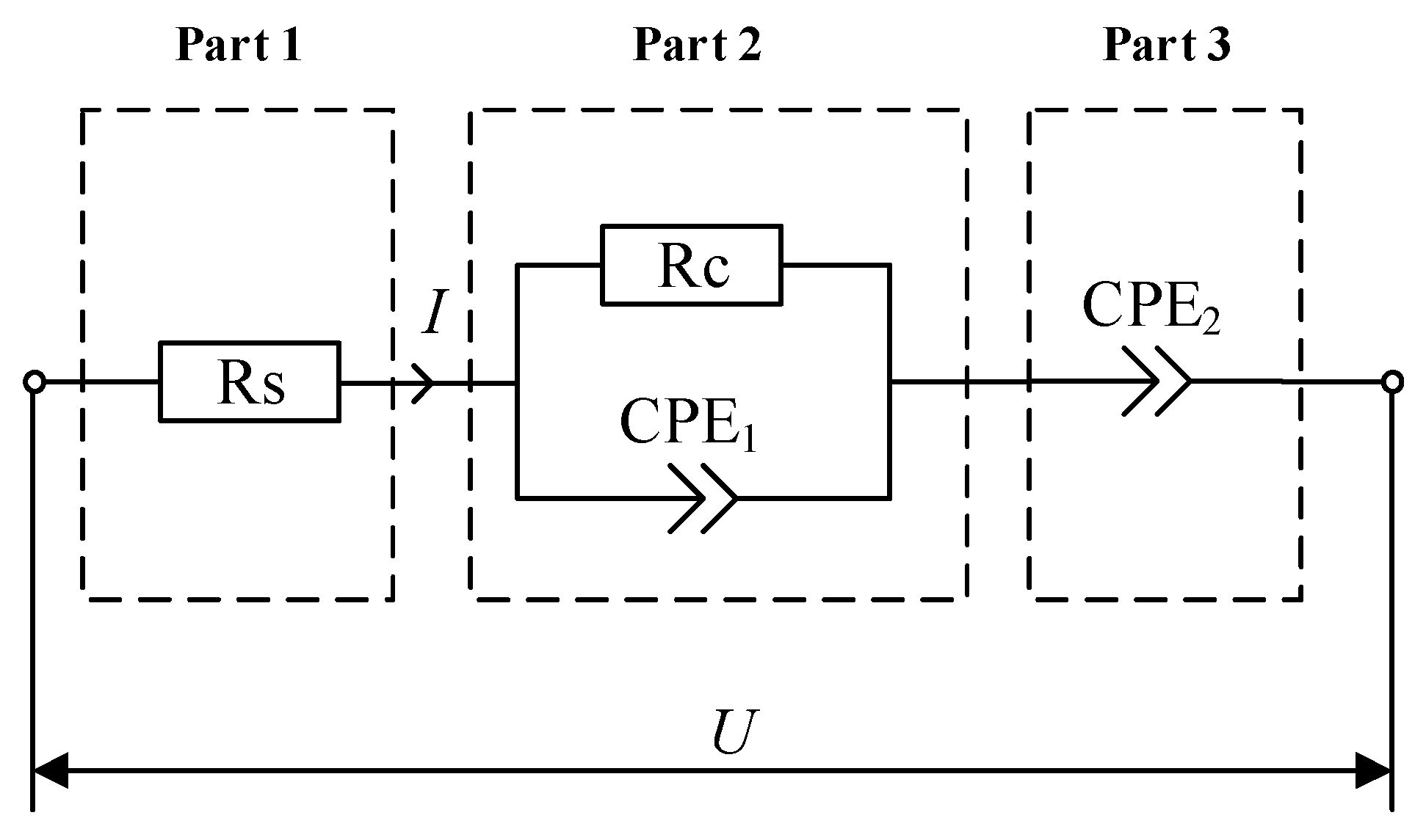
4.1. Fractional Order Modeling of UC

UC, also known as electrochemical double layer capacitor, stores the electrical energy by ion absorption in the double-layer or pseudo-capacitive between electrode and electrolyte. A double layer in the order of 0.3–0.8 nm gradually forms during charging or discharging, which leads to a larger capacitance and higher energy density than ordinary capacitors. In addition, carbon with pores is widely used as the electrode of UC because it provides a larger surface area. Because of that energy storage principle and the use of carbon electrodes, UC performance is affected by distributed surface reactivity, inhomogeneity, and roughness, which can be better characterized by CPE according to the electrochemical impedance spectroscopy (EIS). The impedance curve will deflect downward to a squashed semi-circle if the capacitor parallel with the resistor is replaced by CPE. The CPE can also model the imperfect capacitor behavior of a double-layer capacitor; therefore, this paper proposed a fractional model with 2 CPEs as shown in Figure 9.

The impedance of CPEs can be expressed as follows:

$$Z_{CP{E}_1}\left(j\omega \right)=\frac{1}{C_1{\left(j\omega \right)}^{\alpha }}$$

(11)

$$Z_{CP{E}_2}\left(j\omega \right)=\frac{1}{C_2{\left(j\omega \right)}^{\beta }}$$

(12)

where $C_1$ and $C_2$ are the capacitance coefficients, $\alpha \left(0\le \alpha \le 1\right)$ and $\beta \left(0\le \beta \le 1\right)$ are the fractional orders of CPE. According to the equivalent circuit structure, the transfer function of the fractional model can be delineated by the following:

$$G\left(s\right)=\frac{U\left(s\right)}{I\left(s\right)}=R_s+\frac{R_c}{1+C_1{R}_c{s}^{\alpha }}+\frac{1}{C_2{s}^{\beta }}$$

(13)

where $R_s$ represents the series resistance and $R_s$ is particularly small for UC. Part 2 which consists of $CP{E}_1$ and $R_c$ serves to capture the charge diffusion caused by specifically adsorbed ions. $CP{E}_2$ models the behavior of the double layer. To simplify the solving process, the inverse Laplace transformation in Equation (13) can be divided into three parts due to its linear nature:

$$U\left(t\right)=U_1\left(t\right)+U_2\left(t\right)+U_3\left(t\right)$$

(14)

$$\frac{U_1\left(t\right)}{R_s}=I\left(t\right)$$

(15)

$$\frac{U_2\left(t\right)}{R_c}+C_1{D}_t^{\alpha }{U}_2\left(t\right)=I\left(t\right)$$

(16)

$$C_2{D}_t^{\beta }{U}_3\left(t\right)=I\left(t\right)$$

(17)

With the method proposed in [29] by Zhao C.N. and Xue D.Y., the solution to the fractional-order differential equation

$$a_1{D}^{{\gamma }_1}y(t)+a_2{D}^{{\gamma }_2}y(t)+\cdots +a_n{D}^{{\gamma }_n}y(t)=u(t)$$

(18)

can be written as

$$y(t)=\frac{u(t)-{\sum }_{i=1}^n\left(\frac{a_i}{h^{{\gamma }_i}}{\sum }_{j=1}^{\left[\left(t-t_0\right)/h\right]}{\omega }_j^{\left({\gamma }_i\right)}{y}_{t-jh}\right)}{{\sum }_{i=1}^n\frac{a_i}{h^{{\gamma }_i}}}$$

(19)

$${\omega }_0^{\left({\gamma }_i\right)}=1,{\omega }_j^{\left({\gamma }_i\right)}=\left(1-\frac{{\gamma }_i+1}{j}\right){\omega }_{j-1}^{{\gamma }_i}, j=1, 2,\cdots$$

(20)

For part 1: $U_1\left(t\right)=R_s·I\left(t\right)$;

For part 2: $u(t)=I(t)$, $y(t)=U_2(t)$, $a=[\begin{array}{cc}{C}_1& \frac{1}{R_c}\end{array}]$, $\gamma =\left[\begin{array}{cc}\alpha & 0\end{array}\right]$;

For part 3: $u(t)=I(t)$, $y(t)=U_3(t)$, $a=C_2$, $\gamma =\beta$.

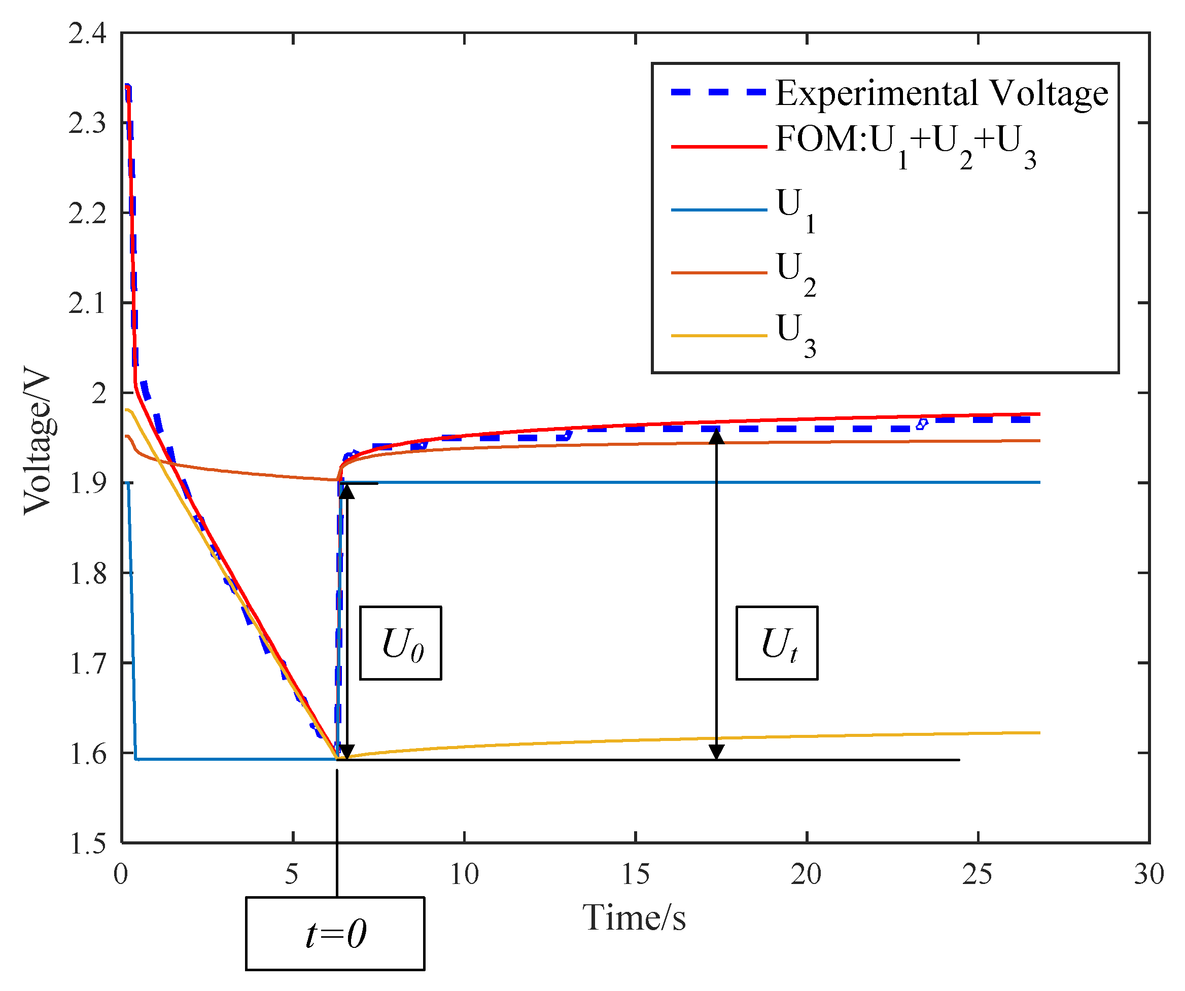
4.2. Time Domain Response Analysis of UC

After the current is set to zero, the terminal voltage of UC varies with the time. This phenomenon is called voltage rebound and can be used to calculate the effective resistance of UC with the formula $R_t=U_t/I$ [30]. The response of Nesscap to a single pulse is drawn in Figure 10. When current is suddenly set to zero, t = 0 and the resistance at this point R₀ = U₀/I. As t increases, $R_t$ increases. If parameters are assigned values: $R_s=1.537 \mathrm{m}\mathsf{\Omega }$, $R_c=5.393 \mathrm{m}\mathsf{\Omega }$, $C_1=7501 \mathrm{F}$, $C_1=2918 \mathrm{F}$, $\alpha =0.2699$, $\beta =0.9663$, the model response fits well with the real response. Decompose the model response into three parts, as shown in Figure 10, according to the previous section. $U_1$ imitates the immediate resistance rebound at t = 0 and equals to U₀, so R_s = R₀. It can be seen both U₂ and U₃ contribute to the response for t > 0 and t < 0. U₂ mainly represents the obvious inertia properties under the sudden current change while U₃ mainly represents the capacitance characteristics. The existence of $\alpha$ and $\beta$ provides a more flexible approach to receive a more accurate model.

The resistance of different voltages at 200 A is calculated by using the same method and its variation with voltage is shown in Figure 11. Charging $R_s$ keeps steady in the charging process. In discharging experiment, $R_s$ increases sharply. In the later parameter identification, $R_s$ is determined by the look-up table method.

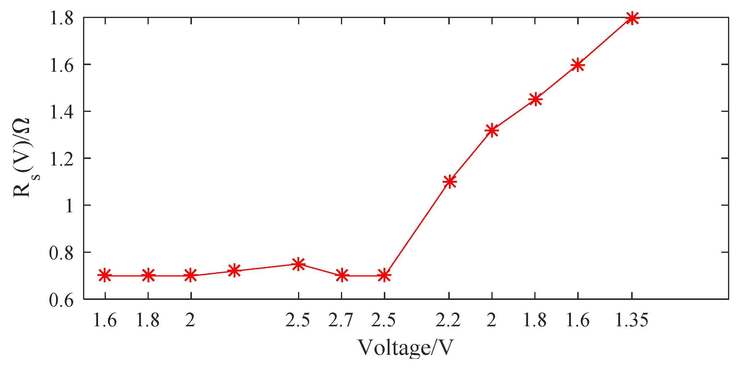
4.3. Parameter Estimation in Time Domain

A Nesscap UC with the nominal capacitance of 3000 F, steady-state resistance of $0.4 \mathrm{m}\mathsf{\Omega }$, power density of 512 W/kg, and energy density of 4.4 Wh/kg is used to carry on charge and discharge experiments at different currents. The rectangular current with an amplitude value of 200 A is the input during charging. When $R_s$ can be determined using the look-up table, the remaining five parameters are identified by NMSA. Its objective function is defined as Equation (21), which can well evaluate the ability of the model to describe the real capacitance behavior. U(t) is the measured voltage and $\widehat{U}(t)$ is the derived result from identified model. Sampling time $t=0.1 \mathrm{s}$. The key parameters of NMSA are as follows: population size S = 20, number of searching days g = 100, dimension of map is 5, reflection factor α = 1, expansion factor β = 2, contraction factor γ = 0.5, shrinkage factor δ = 0.5.

$$fitness=\sqrt{\frac{{\sum }_{j=1}^{\left[\left(t_{end}-t_0\right)/h\right]}\left(U(j)-\widehat{U}(j)\right)}{\left[\left(t_{end}-t_0\right)/h\right]}}$$

(21)

5. Results and Discussion

After performing the optimization procedure, the result is $R_c=14.31 \mathrm{m}\mathsf{\Omega }$, $C_1=7021 \mathrm{F}$, $C_2=3799 \mathrm{F}$, $\alpha =0.7944$, $\beta =0.9994$ for charging. The validation test has been done with charging and discharging currents at levels of 300 A and 400 A. The UC voltage is constrained to vary in the voltage range [1.35 V, 2.7 V]. The results are presented in Figure 12. Compared to the fitness results obtained by NMSA without considering the voltage dependence of $R_s$, great improvement was achieved under a discharge condition. The error between Nesscap and the nonlinear model is within 0.02 V for charging and 0.05 V for discharging. The result shows that the model gives an accurate voltage response for 300 A and 400 A current level. Though there is a slight difference between the charging and discharging, which may be caused by changes in other parameters, it can be neglected. The proposed model simulates UC behavior with good accuracy in the time domain.

6. Conclusions

In this paper, a fractional model of UC is applied. The influence of two fractional parameters $\alpha \left(0\le \alpha \le 1\right)$ and $\beta \left(0\le \beta \le 1\right)$ on the UC model’s time domain is analyzed. $\alpha$ represents the inertia properties in UC, $\beta$ represents the undesirable components in UC. The voltage dependence of $R_s$ is discussed and a look-up table is set up to add nonlinear characteristics to the model using the voltage rebound method. The resistance of UC varies greatly during discharging. A new hybrid optimization algorithm NMSA is proposed in this paper and has been proven to have sufficient global search capability and accuracy. After applying 300 A and 400 A level current to the identified model, it can be proved that the current magnitude and status of charging or discharging have almost no influence or slight influence on the UCs behavior in the range [200 A, 400 A].

References

1. Kurra, N.; Jiang, Q.; Alshareef, H.N. A general strategy for the fabrication of high performance microsupercapacitors. Nano Energy 2015, 16, 1–9. [Google Scholar] [CrossRef] [Green Version]
2. Ladrón de Guevara, A.; Boscá, A.; Pedrós, J.; Climent-Pascual, E.; de Andrés, A.; Calle, F.; Martínez, J. Reduced Graphene oxide/polyaniline electrochemical supercapacitors fabricated by laser. Appl. Surf. Sci. 2019, 467, 691–697. [Google Scholar] [CrossRef]
3. Conway, B.E. Electrochemical Supercapacitors: Scientific Fundamentals and Technological Applications, 1st ed.; Springer Science & Business Media: New York, NY, USA, 2013; pp. 11–31. [Google Scholar]
4. Oldham, K.B. A Gouy–Chapman–Stern model of the double layer at a (metal)/(ionic liquid) interface. J. Electroanal. Chem. 2008, 613, 131–138. [Google Scholar] [CrossRef]
5. Staser, J.A.; Weidner, J.W. Mathematical modeling of hybrid asymmetric electrochemical capacitors. J. Electrochem. Soc. 2014, 161, E3267–E3275. [Google Scholar] [CrossRef]
6. Eddahech, A.; Ayadi, M.; Briat, O.; Vinassa, J.-M. Multilevel neural-network model for supercapacitor module in automotive applications. In Proceedings of the 4th International Conference on Power Engineering, Energy and Electrical Drives, Istanbul, Turkey, 13–17 May 2013; pp. 1460–1465. [Google Scholar]
7. Zhu, S.; Li, J.; Ma, L.; He, C.; Liu, E.; He, F.; Shi, C.; Zhao, N. Artificial neural network enabled capacitance prediction for carbon-based supercapacitors. Mater. Lett. 2018, 233, 294–297. [Google Scholar] [CrossRef]
8. Ma, H.; Wang, B.; Liu, K.R. Distributed Signal Compressive Quantization and Parallel Interference Cancellation for Cloud Radio Access Network. IEEE Trans. Commun. 2018, 66, 4186–4198. [Google Scholar] [CrossRef]
9. Spyker, R.L.; Nelms, R.M. Classical equivalent circuit parameters for a double-layer capacitor. IEEE Trans. Aerosp. Electron. Syst. 2000, 36, 829–836. [Google Scholar] [CrossRef]
10. Zubieta, L.; Bonert, R. Characterization of double-layer capacitors for power electronics applications. IEEE Trans. Ind. Applicat. 2000, 36, 199–205. [Google Scholar] [CrossRef]
11. Itagaki, M.; Suzuki, S.; Shitanda, I.; Watanabe, K.; Nakazawa, H. Impedance analysis on electric double layer capacitor with transmission line model. J. Power Sources 2007, 164, 415–424. [Google Scholar] [CrossRef]
12. Freeborn, T.J.; Maundy, B.; Elwakil, A.S. Fractional-order models of supercapacitors, batteries and fuel cells: A survey. Mater. Renew. Sustain. Energy 2015, 4, 9. [Google Scholar] [CrossRef]
13. Bertrand, N.; Sabatier, J.; Briat, O.; Vinassa, J.-M. Embedded fractional nonlinear supercapacitor model and its parametric estimation method. IEEE Trans. Ind. Electron. 2010, 57, 3991–4000. [Google Scholar]
14. Li, M.; Liu, X. The least squares based iterative algorithms for parameter estimation of a bilinear system with autoregressive noise using the data filtering technique. Signal Process. 2018, 147, 23–34. [Google Scholar] [CrossRef]
15. Ding, F.; Chen, H.; Xu, L.; Dai, J.; Li, Q.; Hayat, T. A hierarchical least squares identification algorithm for Hammerstein nonlinear systems using the key term separation. J. Frankl. Inst. 2018, 355, 3737–3752. [Google Scholar] [CrossRef]
16. Spendley, W.; Hext, G.R.; Himsworth, F.R. Sequential application of simplex designs in optimisation and evolutionary operation. Technometrics 1962, 4, 441–461. [Google Scholar] [CrossRef]
17. Nazareth, L.; Tseng, P. Gilding the lily: A variant of the Nelder-Mead algorithm based on golden-section search. Comput. Optim. Appl. 2002, 22, 133–144. [Google Scholar] [CrossRef]
18. Sun, J.; Zhao, J.; Wu, X.; Fang, W.; Cai, Y.; Xu, W. Parameter estimation for chaotic systems with a drift particle swarm optimization method. Phys. Lett. A 2010, 374, 2816–2822. [Google Scholar] [CrossRef]
19. Zhang, L.; Hu, X.; Wang, Z.; Sun, F.; Dorrell, D.G. Fractional-order modeling and State-of-Charge estimation for ultracapacitors. J. Power Sources 2016, 314, 28–34. [Google Scholar] [CrossRef]
20. Li, X.; Yin, M. Parameter estimation for chaotic systems by hybrid differential evolution algorithm and artificial bee colony algorithm. Nonlinear Dyn. 2014, 77, 61–71. [Google Scholar] [CrossRef]
21. Dai, C.; Chen, W.; Cheng, Z.; Li, Q.; Jiang, Z.; Jia, J. Seeker optimization algorithm for global optimization: A case study on optimal modelling of proton exchange membrane fuel cell (PEMFC). J. Electr. Power 2011, 33, 369–376. [Google Scholar] [CrossRef]
22. Ketabi, A.; Sheibani, M.R.; Nosratabadi, S.M. Power quality meters placement using seeker optimization algorithm for harmonic state estimation. J. Electr. Power 2012, 43, 141–149. [Google Scholar] [CrossRef]
23. Kumar, M.R.; Deepak, V.; Ghosh, S. Fractional-order controller design in frequency domain using an improved nonlinear adaptive seeker optimization algorithm. Turk. J. Electr. Eng. Comput. 2017, 25, 4299–4310. [Google Scholar] [CrossRef]
24. Ross, B. A brief history and exposition of the fundamental theory of fractional calculus. In Fractional Calculus and Its Applications, 1st ed.; Ross, B., Ed.; Springer: Berlin, German, 1975; Volume 457, pp. 1–36. [Google Scholar]
25. Monje, C.A.; Chen, Y.; Vinagre, B.M.; Xue, D.; Feliu-Batlle, V. Fractional-Order Systems and Controls: Fundamentals and Applications, 1st ed.; Springer Science & Business Media: London, UK, 2010; pp. 9–34. [Google Scholar]
26. Dzieliński, A.; Sierociuk, D.; Sarwas, G. Some applications of fractional order calculus. Bull. Pol. Acad. Sci. Tech. Sci. 2010, 58, 583–592. [Google Scholar] [CrossRef] [Green Version]
27. Mühlenbein, H.; Schomisch, M.; Born, J. The parallel genetic algorithm as function optimizer. Parallel Comput. 1991, 17, 619–632. [Google Scholar] [CrossRef]
28. Thomas, B. Evolutionary Algorithms in Theory and Practice: Evolution Strategies, Evolutionary Programming, Genetic Algorithms, 1st ed.; Oxford University Press: New York, NY, USA, 1996; pp. 137–159. [Google Scholar]
29. Xue, D.; Bai, L. Numerical algorithms for Caputo fractional-order differential equations. Int. J. Control 2017, 90, 1201–1211. [Google Scholar] [CrossRef]
30. Zhao, J.; Gao, Y.; Burke, A.F. Performance testing of supercapacitors: Important issues and uncertainties. J. Power Sources 2017, 363, 327–340. [Google Scholar] [CrossRef]
Figure 1. Determine the search direction.
Energies 12 04251 g001
Figure 2. Determine the search step length.
Energies 12 04251 g002
Figure 3. NM evolutionary process.
Energies 12 04251 g003
Figure 4. NM algorithm.
Energies 12 04251 g004
Figure 5. A case of NM algorithm.
Energies 12 04251 g005
Figure 6. NMSA algorithm.
Energies 12 04251 g006
Figure 7. Visualization of Rastrigin function.
Energies 12 04251 g007
Figure 8. The Fitness curve of the seeker optimization algorithm (SOA) and NMSA; (a) is the fitness curve of SOA; (b) is the fitness curve of NMSA.
Energies 12 04251 g008
Figure 9. Ultracapacitor (UC) fractional model.
Energies 12 04251 g009
Figure 10. Single-pulse response of UC.
Energies 12 04251 g010
Figure 11. Resistance variation at 200 A.
Energies 12 04251 g011
Figure 12. Comparison between model voltage response and UC voltage (The left side is the response curve and the right side it the response error compared with UC voltage) (a) Validation test with 300 A charging profile; (b) Validation test with 400 A charging profile; (c) Validation test with 300 A discharging profile; (d) Validation test with 400 A discharging profile.
Energies 12 04251 g012aEnergies 12 04251 g012b