Thermodynamic Performance of a Double-Effect Absorption Refrigeration Cycle Based on a Ternary Working Pair: Lithium Bromide + Ionic Liquids + Water

Abstract
:
1. Introduction
2. Measuring Method and Thermodynamic Properties
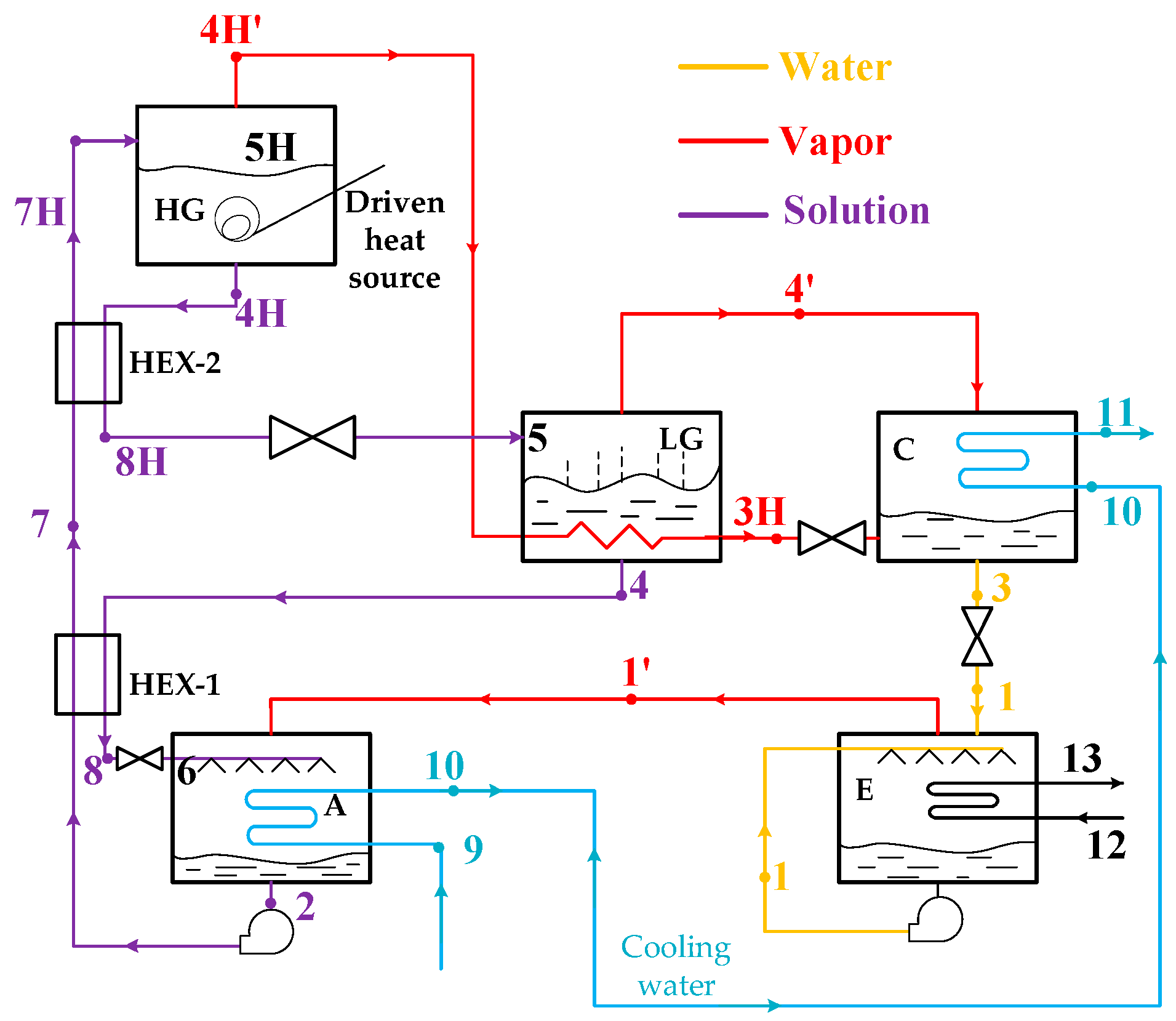
3. Thermodynamic Analysis of a Double-Effect Absorption Refrigeration Cycle
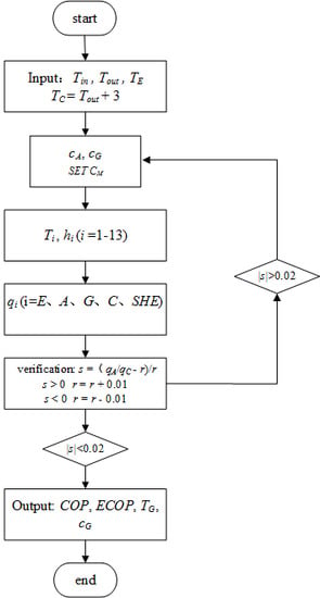
3.1. Thermodynamic Calculation
- The cycle is under a steady state.
- The kinetic and potential energies are negligible.
- Enthalpy of the fluid does not change when flowing through the expansion valve.
- The refrigerant leaving the condenser is saturated liquid.
- The refrigerant leaving the evaporator is saturated vapor.
3.2. Thermodynamic Calculation Results
3.3. Thermodynamic Analysis and Discussion
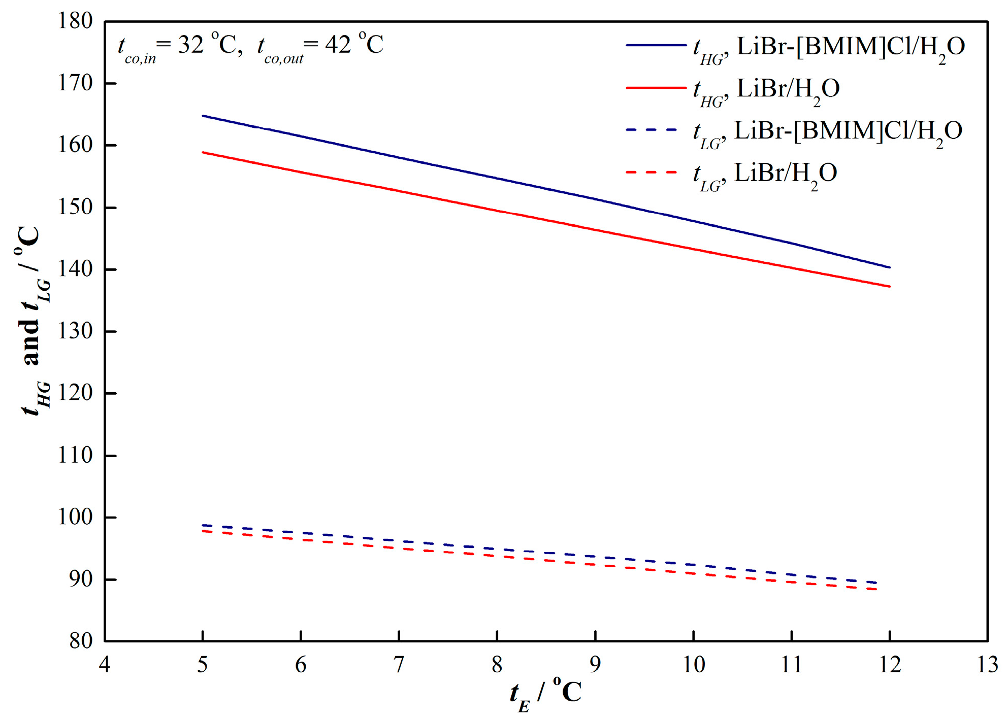
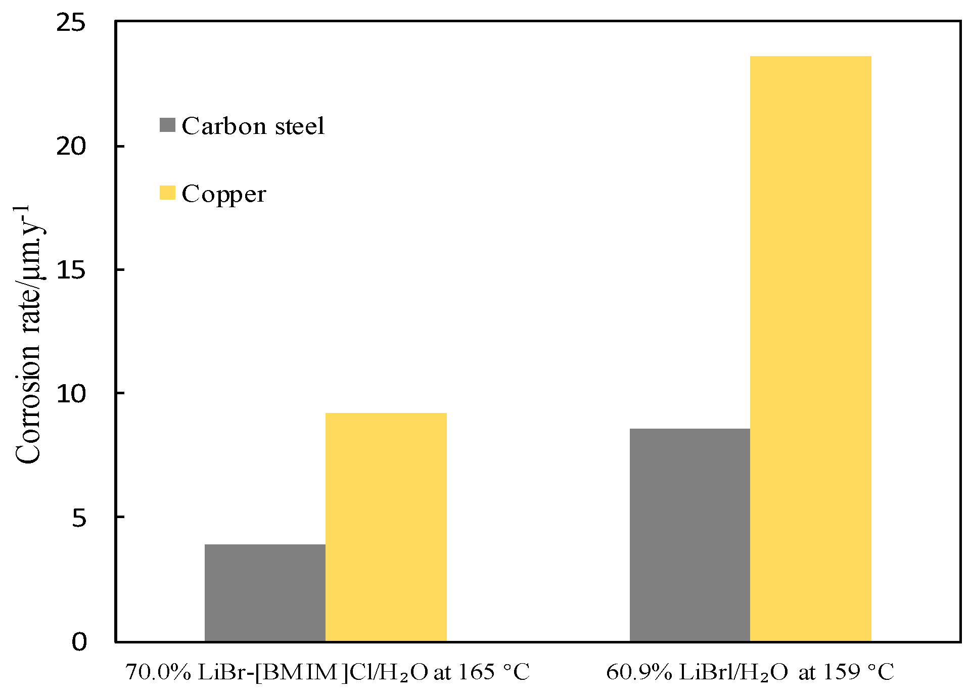
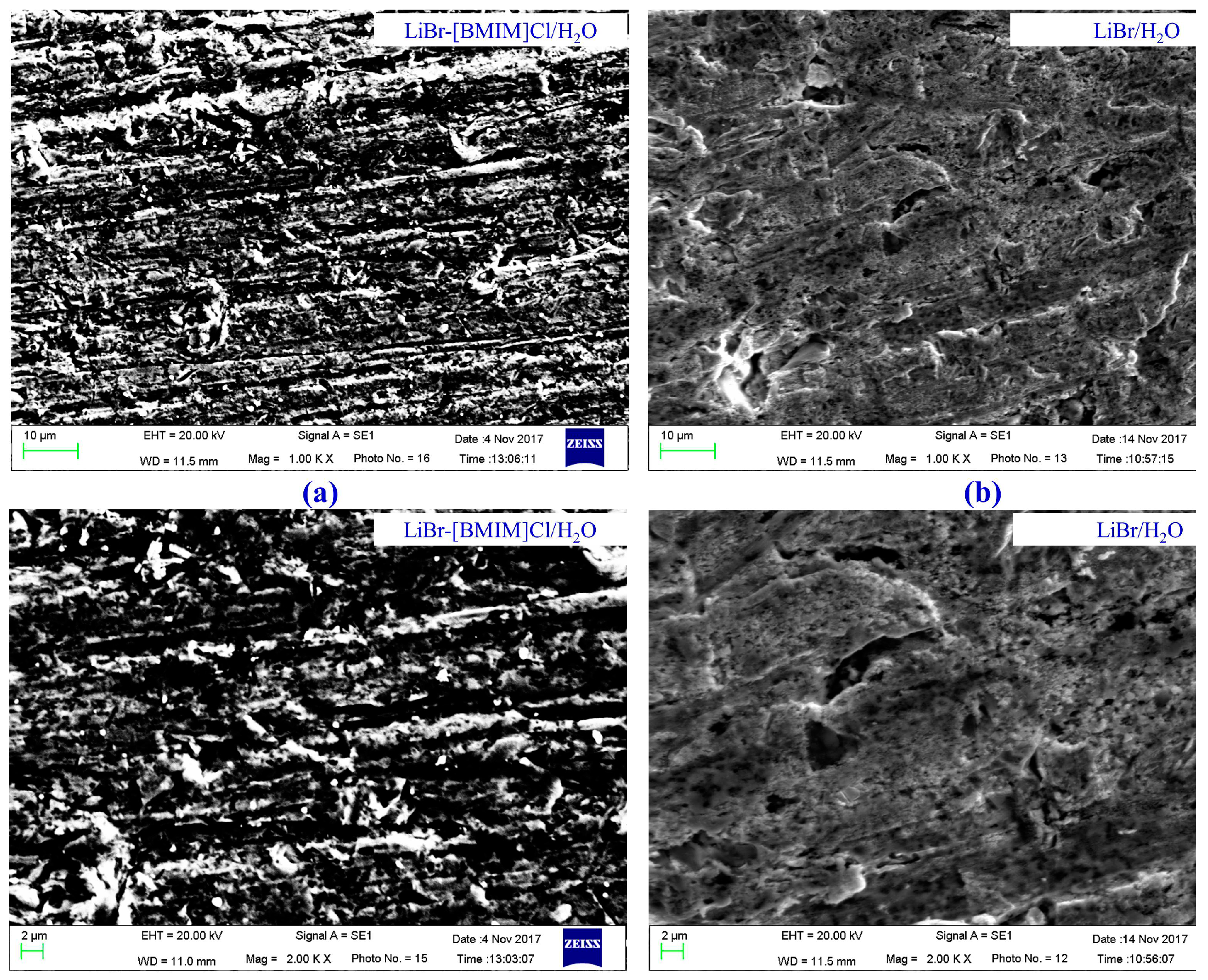
3.3.1. Generation Temperature and Corrosion
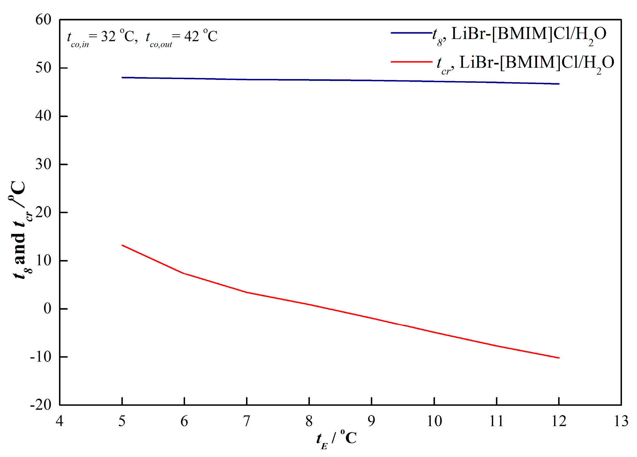
3.3.2. Crystallization Problem
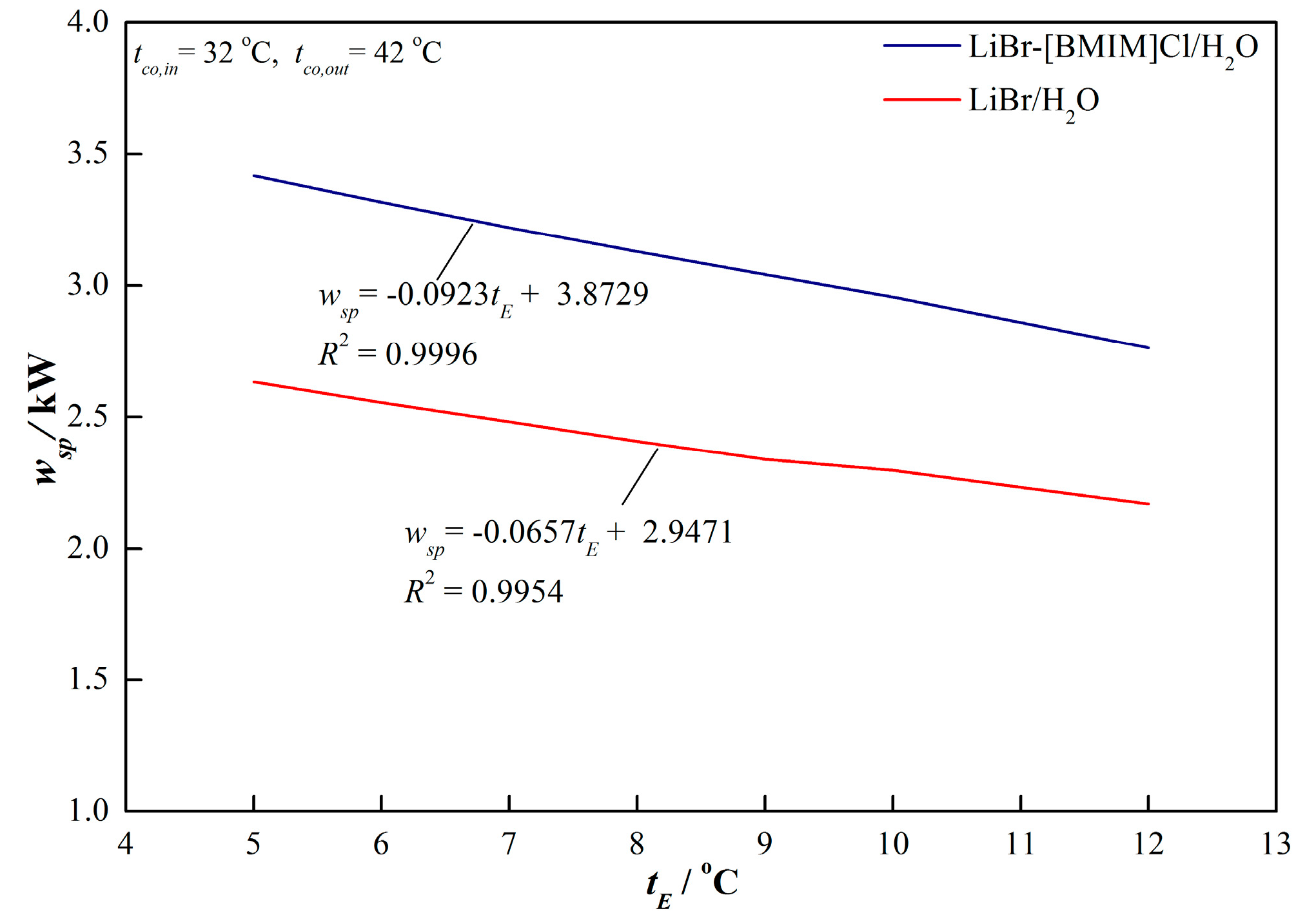
3.3.3. Solution Pump Power
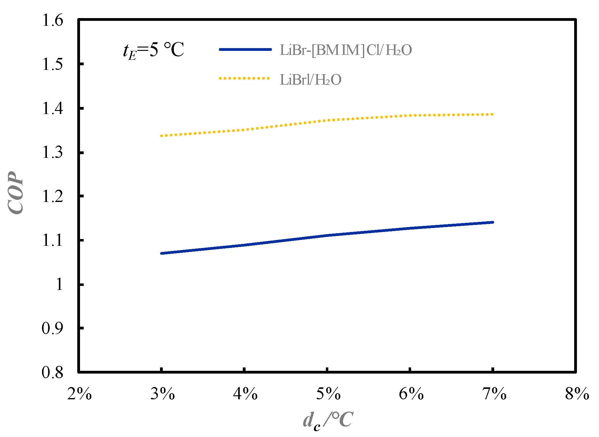
3.3.4. COPc
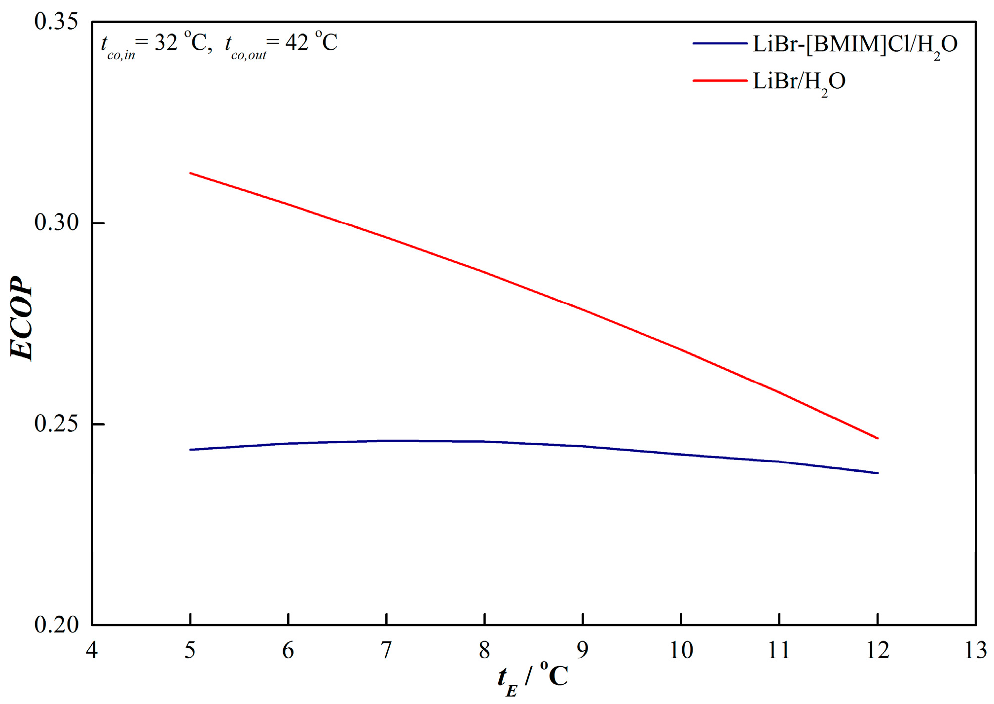
3.3.5. ECOPc
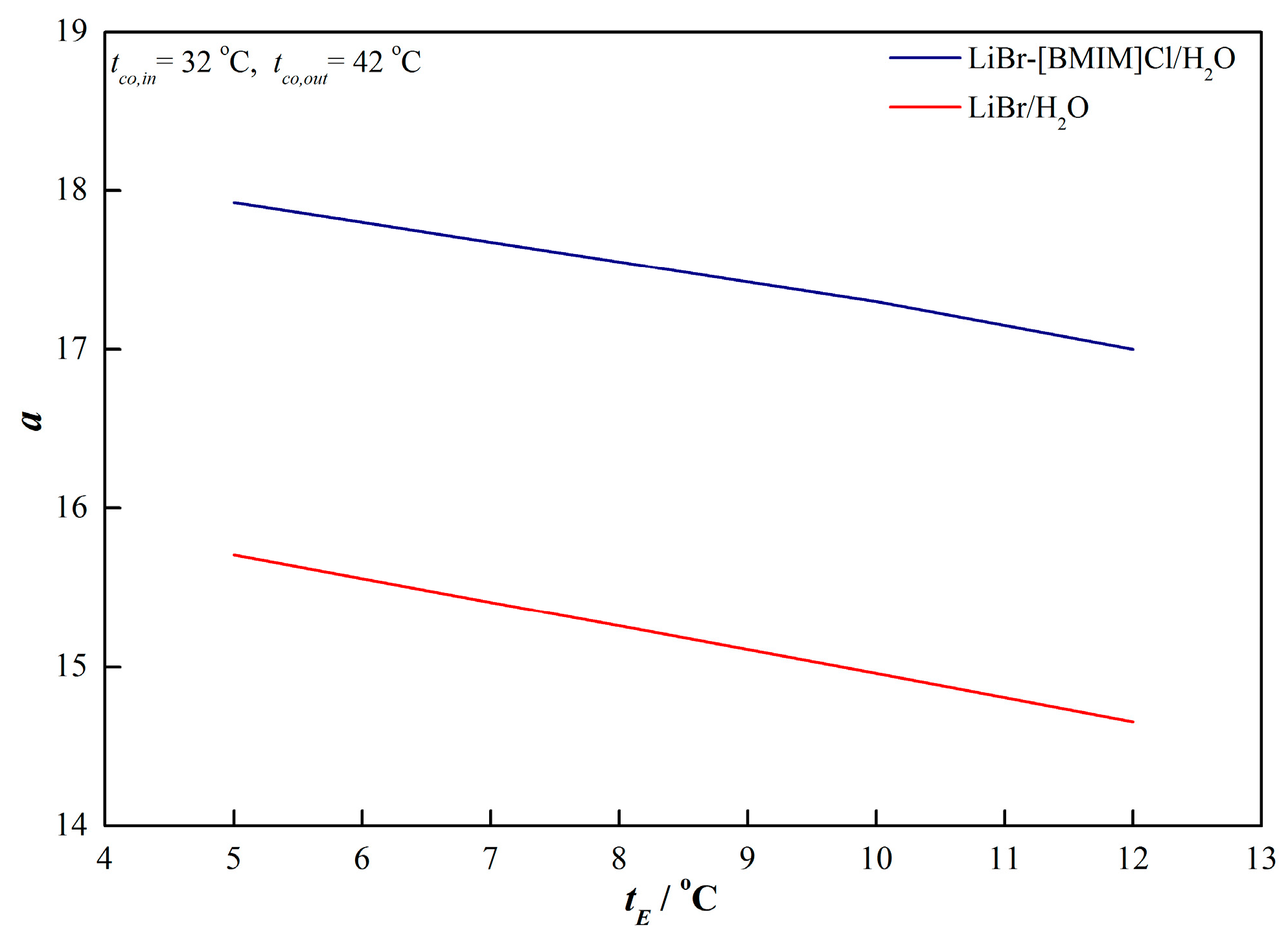
3.3.6. Concentration Difference between Weak and Strong Solution
4. Conclusions
Author Contributions
Funding
Conflicts of Interest
Nomenclature
| [BMIM]Cl | 1-butyl-3-methylimidazolium chloride |
| a | circulation ratio |
| COPc | coefficient of performance |
| Cp | specific heat capacity, J·g−1·K−1 |
| ECOPc | exergy coefficient of performance |
| h | specific enthalpy, kJ·kg−1 |
| ILs | ionic liquids |
| m | mass flow rate of the solution, kg·s−1 |
| p | vapor pressure, kPa |
| q | specific heat load, kJ·s−1 |
| Re | Reynolds number |
| T | temperature, K |
| t | temperature, °C |
| w | mass fraction of absorbent |
| η | efficiency |
| ν | viscosity, mm2·s−1 |
| ρ | density, g·cm−3 |
| λ | frictional factor |
| ζ | factor of local resistance |
| θ | Carnot factor |
| A | absorber |
| C | condenser |
| cr | crystallization |
| E | evaporator |
| HEX-1, HEX-2 | solution heat exchanger |
| HG | high-pressure generator |
| LG | low-pressure generator |
| sp | solution pump |
Appendix A

| T (K) | p (kPa) | T (K) | p (kPa) | T (K) | p (kPa) | T (K) | p (kPa) |
|---|---|---|---|---|---|---|---|
| w1+2 = 0.60 | w1+2 = 0.65 | w1+2 = 0.70 | w1+2 = 0.75 | ||||
| 296.4 | 0.71 | 309.7 | 0.82 | 303.7 | 0.55 | 356.7 | 2.90 |
| 316.4 | 2.06 | 323.3 | 1.70 | 313.4 | 0.96 | 367.5 | 4.89 |
| 326.7 | 3.69 | 334.3 | 3.00 | 323.8 | 1.51 | 379.0 | 8.35 |
| 336.5 | 5.98 | 345.9 | 5.57 | 332.4 | 2.91 | 389.5 | 12.77 |
| 346.7 | 9.69 | 355.9 | 8.85 | 345.1 | 4.86 | 399.8 | 19.03 |
| 357.8 | 15.28 | 365.3 | 13.34 | 355.3 | 7.80 | 410.4 | 27.76 |
| 367.5 | 22.05 | 375.2 | 19.82 | 364.7 | 12.57 | 420.3 | 38.98 |
| 377.8 | 32.60 | 384.5 | 28.22 | 375.1 | 18.59 | 429.9 | 56.05 |
| 388.6 | 48.40 | 395.8 | 41.96 | 384.8 | 28.815 | 441.6 | 76.89 |
| 400.2 | 71.00 | 405.7 | 59.23 | 396.5 | 40.84 | 449.6 | 98.50 |
| 408.7 | 92.65 | 415.4 | 79.80 | 405.6 | 58.25 | ||
| 423.2 | 100.70 | 416.5 | 79.00 | ||||
| i | Ai | Bi | Ci |
|---|---|---|---|
| 0 | −1.0265478 | 39.616964 | 210.51137 |
| 1 | 0.74875570 | −549.1808 | −302.38069 |
| 2 | −1.2196498 × 10⁻² | 18.494558 | −594.34163 |
| 3 | −1.2684596 × 10⁻⁴ | 4.44125×10⁻¹⁹ | −3.1545374 |
| 4 | 1.5837523 × 10⁻⁶ | −6.24780×10⁻⁴ | −306.48281 |
| T (K) | ρ (g·cm−3) | T (K) | ρ (g·cm−3) | T (K) | ρ (g·cm−3) | T (K) | ρ (g·cm−3) | T (K) | ρ (g·cm−3) |
|---|---|---|---|---|---|---|---|---|---|
| w1+2 = 0.55 | w1+2 = 0.60 | w1+2 = 0.65 | w1+2 = 0.70 | w1+2 = 0.75 | |||||
| 303.15 | 1.384 | 303.15 | 1.434 | 303.15 | 1.49 | 303.15 | 1.549 | ||
| 313.15 | 1.378 | 313.15 | 1.428 | 313.15 | 1.483 | 313.15 | 1.542 | ||
| 323.15 | 1.372 | 323.15 | 1.422 | 323.15 | 1.477 | 323.15 | 1.535 | ||
| 333.15 | 1.367 | 333.15 | 1.416 | 333.15 | 1.47 | 333.15 | 1.528 | 333.15 | 1.59 |
| 343.15 | 1.361 | 343.15 | 1.411 | 343.15 | 1.464 | 343.15 | 1.521 | 343.15 | 1.582 |
| 353.15 | 1.355 | 353.15 | 1.405 | 353.15 | 1.458 | 353.15 | 1.515 | 353.15 | 1.575 |
| 363.15 | 1.349 | 363.15 | 1.399 | 363.15 | 1.452 | 363.15 | 1.508 | 363.15 | 1.568 |
| 373.15 | 1.343 | 373.15 | 1.393 | 373.15 | 1.446 | 373.15 | 1.502 | 373.15 | 1.561 |
| i | Ai | Bi (×10−3) | Ci (×10−5) |
|---|---|---|---|
| 0 | 0.384514 | 6.128884 | −1.221983 |
| 1 | 2.024635 | −16.63302 | 3.272392 |
| 2 | 8.490245 × 10⁻² | 8.778485 | −2.017801 |
| T (K) | ν (mm2·s−1) | T (K) | ν (mm2·s−1) | T (K) | ν (mm2·s−1) | T (K) | ν (mm2·s−1) | T (K) | ν (mm2·s−1) |
|---|---|---|---|---|---|---|---|---|---|
| w1+2 = 0.55 | w1+2 = 0.60 | w1+2 = 0.65 | w1+2 = 0.70 | w1+2 = 0.75 | |||||
| 303.15 | 3.81 | 303.15 | 6.21 | 303.15 | 10.31 | 303.15 | 23.01 | ||
| 313.15 | 3.01 | 313.15 | 4.88 | 313.15 | 7.82 | 313.15 | 16.13 | ||
| 323.15 | 2.44 | 323.15 | 3.87 | 323.15 | 6.02 | 323.15 | 11.61 | ||
| 333.15 | 1.99 | 333.15 | 3.06 | 333.15 | 4.66 | 333.15 | 8.39 | 333.15 | 21.29 |
| 343.15 | 1.68 | 343.15 | 2.49 | 343.15 | 3.71 | 343.15 | 6.35 | 343.15 | 14.14 |
| 353.15 | 1.46 | 353.15 | 2.11 | 353.15 | 3.05 | 353.15 | 4.94 | 353.15 | 10.00 |
| 363.15 | 1.30 | 363.15 | 1.83 | 363.15 | 2.60 | 363.15 | 4.03 | 363.15 | 7.46 |
| 373.15 | 1.18 | 373.15 | 1.63 | 373.15 | 2.22 | 373.15 | 3.34 | 373.15 | 5.81 |
| i | Ai (×102) | Bi (×104) | Ci (×106) |
|---|---|---|---|
| 0 | 1.217521 | −5.828088 | 3.460217 |
| 1 | −3.896274 | 13.818580 | 8.897532 |
| 2 | 3.291964 | −1.092322 | −51.704210 |
| 3 | −0.295650 | −9.908650 | 46.722780 |
| T (K) | Cp (J·g−1·K−1) | T (K) | Cp (J·g−1·K−1) | T (K) | Cp (J·g−1·K−1) | T (K) | Cp (J·g−1·K−1) | T (K) | Cp (J·g−1·K−1) |
|---|---|---|---|---|---|---|---|---|---|
| w1+2 = 0.55 | w1+2 = 0.60 | w1+2 = 0.65 | w1+2 = 0.70 | w1+2 = 0.75 | |||||
| 303.15 | 2.30 | 303.15 | 2.20 | 303.15 | 2.05 | 303.15 | 1.94 | ||
| 313.15 | 2.32 | 313.15 | 2.21 | 313.15 | 2.07 | 313.15 | 1.96 | ||
| 323.15 | 2.33 | 323.15 | 2.22 | 323.15 | 2.08 | 323.15 | 1.96 | ||
| 333.15 | 2.34 | 333.15 | 2.22 | 333.15 | 2.10 | 333.15 | 1.97 | 333.15 | 1.85 |
| 343.15 | 2.35 | 343.15 | 2.23 | 343.15 | 2.11 | 343.15 | 1.98 | 343.15 | 1.86 |
| 353.15 | 2.38 | 353.15 | 2.24 | 353.15 | 2.12 | 353.15 | 2.01 | 353.15 | 1.88 |
| 363.15 | 2.40 | 363.15 | 2.27 | 363.15 | 2.16 | 363.15 | 2.03 | 363.15 | 1.91 |
| 373.15 | 2.45 | 373.15 | 2.30 | 373.15 | 2.19 | 373.15 | 2.07 | 373.15 | 1.93 |
| i | Ai | Bi (×10−2) | Ci (×10−5) |
|---|---|---|---|
| 0 | 4.656718 | −1.447759 | 3.392384 |
| 1 | 3.182206 | −1.114172 | −1.471251 |
| 2 | −6.925005 | 2.383878 | −1.126738 |
| 283.15 K | 293.15 K | 303.15 K | 313.15 K | 323.15 K | 333.15 K | 343.15 K | 353.15 K | 363.15 K | 373.15 K |
|---|---|---|---|---|---|---|---|---|---|
| 1.55 | 1.62 | 1.73 | 1.94 | 2.55 | 6.31 | 1.98 | 1.98 | 2.025 | 2.05 |
| Mass fraction | 0.55 | 0.60 | 0.65 | 0.70 |
|---|---|---|---|---|
| Dissolution enthalpy/kJ·kg−1 | −160.66 | −173.93 | −189.89 | −168.04 |
| T (K) | h(kJ·kg−1) | T (K) | h(kJ·kg−1) | T (K) | h (kJ·kg−1) | T (K) | h (kJ·kg−1) |
|---|---|---|---|---|---|---|---|
| w1+2 = 0.55 | w1+2 = 0.60 | w1+2 = 0.65 | w1+2 = 0.70 | ||||
| 303.15 | 331.04 | 303.15 | 312.51 | 303.15 | 291.33 | 303.15 | 307.99 |
| 313.15 | 354.18 | 313.15 | 334.45 | 313.15 | 312.04 | 313.15 | 327.44 |
| 323.15 | 377.38 | 323.15 | 356.45 | 323.15 | 332.82 | 323.15 | 346.97 |
| 333.15 | 400.70 | 333.15 | 378.56 | 333.15 | 353.70 | 333.15 | 366.60 |
| 343.15 | 424.17 | 343.15 | 400.81 | 343.15 | 374.72 | 343.15 | 386.39 |
| 353.15 | 447.84 | 353.15 | 423.24 | 353.15 | 395.92 | 353.15 | 406.35 |
| 363.15 | 471.75 | 363.15 | 445.91 | 363.15 | 417.34 | 363.15 | 426.54 |
| 373.15 | 495.96 | 373.15 | 468.84 | 373.15 | 439.01 | 373.15 | 446.98 |
| i | Ai | Bi | Ci | Di |
|---|---|---|---|---|
| 0 | −1.184934 × 10⁴ | 5.791208 × 10⁴ | −9.675233 × 10⁴ | 5.399248 × 10⁴ |
| 1 | 7.876601 × 10⁻¹ | 4.862318 | −5.643877 | 2.016601 × 10⁻³ |
| 2 | 4.233235 × 10⁻³ | −1.054922 × 10⁻² | 8.114677 × 10⁻³ | −2.862036 × 10⁻⁶ |
References
- Ziegler, F.; Kahn, R.; Summerer, F.; Alefeld, G. Multi-effect absorption chillers. Int. J. Refrig. 1993, 16, 301–311. [Google Scholar] [CrossRef]
- Misra, R.D.; Sahoo, P.K.; Gupta, A. Thermoeconomic evaluation and optimization of a double-effect H2O/LiBr vapour-absorption refrigeration system. Int. J. Refrig. 2005, 28, 331–343. [Google Scholar] [CrossRef]
- Gomri, R.; Hakimi, R. Second law analysis of double-effect vapour absorption cooler system. Energy Convers. Manag. 2008, 49, 3343–3348. [Google Scholar] [CrossRef]
- Gomri, R. Second law comparison of single effect and double-effect vapour absorption refrigeration systems. Energy Convers. Manag. 2009, 50, 1279–1287. [Google Scholar] [CrossRef]
- Kaushik, S.C.; Arora, A. Energy and exergy analysis of single effect and series flow double-effect water–lithium bromide absorption refrigeration systems. Int. J. Refrig. 2009, 32, 1247–1258. [Google Scholar] [CrossRef]
- Farshi, L.G.; Mahmoudi, S.M.S.; Rosen, M.A. Exergoeconomic comparison of double-effect and combined ejector-double-effect absorption refrigeration systems. Appl. Energy 2013, 103, 700–711. [Google Scholar] [CrossRef]
- Avanessian, T.; Ameri, M. Energy, exergy, and economic analysis of single and double effect LiBr-H2O absorption chillers. Energy Build. 2014, 73, 26–36. [Google Scholar] [CrossRef]
- Kaynakli, O.; Saka, K.; Kaynakli, F. Energy and exergy analysis of a double effect absorption refrigeration system based on different heat sources. Energy Convers. Manag. 2015, 106, 21–30. [Google Scholar] [CrossRef]
- Tanno, K.; Itoh, M.; Sekiya, H.; Yashiro, H.; Kumagai, N. The corrosion inhibition of carbon steel in lithium bromide solution by hydroxide and molybdate at moderate temperatures. Corros. Sci. 1993, 34, 1453–1461. [Google Scholar] [CrossRef]
- Muñoz, A.I.; García-Antón, J.; Guiñón, J.L.; Herranz, V.P. Comparison of inorganic inhibitors of copper, nickel and copper-nickels in aqueous lithium bromide solution. Electrochim. Acta 2004, 50, 957–966. [Google Scholar] [CrossRef]
- García-García, D.M.; García-Antón, J.; Igual-Muñoz, A.; Blasco-Tamarit, E. Effect of cavitation on the corrosion behaviour of welded and non-welded duplex stainless steel in aqueous LiBr solutions. Corros. Sci. 2006, 48, 2380–2405. [Google Scholar] [CrossRef]
- Hu, X.; Liang, C. Effect of PWVA/Sb2O3 complex inhibitor on the corrosion behavior of carbon steel in 55% LiBr solution. Mater. Chem. Phys. 2008, 110, 285–290. [Google Scholar] [CrossRef]
- Kaneko, M.; Isaacs, H.S. Effects of molybdenum on the pitting of ferritic- and austenitic-stainless steels in bromide and chloride solutions. Corros. Sci. 2002, 44, 1825–1834. [Google Scholar] [CrossRef]
- Muñoz, A.I.; Antón, J.G.; Guiñón, J.L.; Herranz, V.P. Effect of aqueous lithium bromide solutions on the corrosion resistance and galvanic behaveour of copper-nickel alloys. Corrosion 2003, 59, 32–41. [Google Scholar] [CrossRef]
- Guiñón-Pina, V.; Igual-Muñoz, A.; García Antón, J. Influence of PH on the electrochemical behaviour of a duplex stainless steel in highly concentrated LiBr solutions. Corros. Sci. 2011, 53, 575–581. [Google Scholar] [CrossRef]
- Blasco-Tamarit, E.; García-García, D.M.; García-Antón, J. Imposed potential measurements to evaluate the pitting corrosion resistance and the galvanic behaviour of a highly alloyed austenitic stainless steel and its weldment in a LiBr solution at temperatures up to 150 °C. Corros. Sci. 2011, 53, 784–795. [Google Scholar] [CrossRef]
- Sánchez-Tovar, R.; Montañés, M.T.; García-Antón, J. Thermogalvanic corrosion and galvanic effects of copper and AISI 316L stainless steel pairs in heavy LiBr brines under hydrodynamic conditions. Corros. Sci. 2012, 60, 118–128. [Google Scholar] [CrossRef]
- Sun, J.; Fu, L.; Zhang, S. A review of working fluids of absorption cycles. Renew. Sustain. Energy Rev. 2012, 16, 1899–1906. [Google Scholar] [CrossRef]
- Álvarez, M.E.; Esteve, X.; Bourouis, M. Performance analysis of a triple-effect absorption cooling cycle using aqueous (lithium, potassium, sodium) nitrate solution as a working fluid. Appl. Therm. Eng. 2015, 79, 27–36. [Google Scholar] [CrossRef]
- Medrano, M.; Bourouis, M.; Coronas, A. Double-lift absorption refrigeration cycles driven by low-temperature heat sources using organic fluid mixtures as working fluids. Appl. Energy 2001, 68, 173–185. [Google Scholar] [CrossRef]
- Yin, J.; Shi, L.; Zhu, M.S.; Han, L.Z. Performance analysis of an absorption heat transformer with different working fluid combinations. Appl. Energy 2000, 67, 281–292. [Google Scholar] [CrossRef]
- Luo, C.H.; Zhang, Y.; Su, Q.Q. Saturated vapor pressure, crystallization temperature and corrosivity of LiBr-[BMIM]Cl/H2O working pair. CIESC J. 2016, 67, 1110–1116. [Google Scholar]
- Luo, C.H.; Su, Q.Q.; Mi, W.L. Solubilities, vapor pressures, densities, viscosities, and specific heat capacities of the LiNO3/H2O binary system. J. Chem. Eng. Data 2013, 58, 625–633. [Google Scholar] [CrossRef]
- Luo, C.H.; Li, Y.Q.; Chen, K.; Li, N.; Su, Q.Q. Thermodynamic properties and corrosivity of a new absorption heat pump working pair: Lithium nitrate + 1-butyl-3-methylimidazolium bromide + water. Fluid Phase Equilibr. 2017, 451, 25–39. [Google Scholar] [CrossRef]
- Li, Y.Q.; Li, N.; Luo, C.H.; Su, Q.Q. Study on a Quaternary Working Pair of CaCl2-LiNO3-KNO3/H2O for an Absorption Refrigeration Cycle. Entropy 2019, 21, 546. [Google Scholar] [CrossRef]
- Lee, R.J.; DiGuilio, R.M.; Jeter, S.M.; Teja, A.S. Properties of lithium bromide-water solutions at high temperatures and concentrations II: Density and viscosity. ASHRAE Trans. 1990, 96, 709–714. [Google Scholar]
- Iyoki, S.T.; Uemura, T. Heat capacity of water–lithium bromide system and the water-lithium bromide-zinc bromide-lithium chloride system at high temperatures. Int. J. Refrig. 1989, 12, 323–326. [Google Scholar] [CrossRef]
- Wagman, D.D.; Evans, W.H.; Parker, V.B.; Schumm, R.H.; Halow, I.; Bailey, S.M.; Churney, K.L.; Nuttall, R.L. NBS Tables of Chemical Thermodynamic Properties: Selected Values for Inorganic and C1 and C2 Organic Substances in SI Units; The American Chemical Society and the American Institute of Physics for the National Bureau of Standards: Washington DC, USA, 1982. [Google Scholar]
- Kaita, Y. Thermodynamic properties of lithium bromide-water solutions at high temperatures. Int. J. Refrig. 2001, 24, 374–390. [Google Scholar] [CrossRef]
- Liu, G.Q.; Ma, L.X.; Liu, J. Handbook of Chemical and Engineering Property Data: Inorganic Volume, 1st ed.; Chemical Industry Press: Beijing, China, 2006. [Google Scholar]
- Florides, G.A.; Kalogirou, S.A.; Tassou, S.A.; Wrobe, L.C. Design and construction of a LiBr-water absorption machine. Energy Convers. Manag. 2003, 44, 2483–2508. [Google Scholar] [CrossRef]
- Jiang, X.; Cao, Z. A group of simple precise formulations for properties of water and steam. Power Eng. 2003, 23, 2777–2780. [Google Scholar]
- Luo, C.H.; Su, Q.Q. Corrosion of carbon steel in concentrated LiNO3 solution at high temperature. Corros. Sci. 2013, 74, 290–296. [Google Scholar] [CrossRef]


| Reagent | Mass Fraction Purity | Provenance |
|---|---|---|
| [BMIM]Cl a | >0.99 | Shanghai Chengjie Chemical |
| LiBr | >0.995 | Tianjin Jinke Chemical |
| KCl | >0.99 | Sinopharm Chemical Reagent Beijing |
| Li2CrO4 | >0.99 | Tianjin Jinke Chemical |
| Na2SiO3 | >0.995 | Tianjin Guangfu Chemical |
| Polyaspartate | >0.99 | Xiya Chemical |
| Pure water | Home made |
| Refrigeration Conditions | |||
|---|---|---|---|
| Cooling water temperature at inlet | 32 °C | Chilled water temperature at the inlet (t12) | 12 °C |
| Cooling water temperature at outlet | 42 °C | Chilled water temperature at the outlet (t13) | 7 °C |
| Temperature difference at the evaporator | 2 °C | Efficiency of the solution heat exchangers | 0.90 |
| Temperature difference at the absorber, condenser, and generators | 3 °C | Difference of the mass concentration of the both working pairs | 4% |
| Points | Stream | Position | w | t (°C) | p (kPa) | h (kJ·kg−1) | m (kg·s−1) |
|---|---|---|---|---|---|---|---|
| 1′ | Vapor | Outlet of the evaporator | 0 | 5.0 | 0.872 | 2928.53 | 1.00 |
| 1 | Water | Inlet of the evaporator | 0 | 5.0 | 0.872 | 439.63 | 1.00 |
| 2 | Weak solution | Outlet of the absorber | 67.7 | 42.4 | 0.872 | 317.82 | 17.90 |
| 3 | Water | Outlet of the condenser | 0 | 45.0 | 9.58 | 606.99 | 1.00 |
| 3H | Water | Outlet of the low-pressure generator | 0 | 101.8 | 108.52 | 845.47 | 0.60 |
| 4′ | Vapor | Outlet of the low-pressure generator | 0 | 98.8 | 9.58 | 3101.76 | 0.40 |
| 4 | Strong solution | Outlet of the low-pressure generator | 71.7 | 98.8 | 9.58 | 463.13 | 16.90 |
| 4H′ | Vapor | Outlet of the high-pressure generator | 0 | 164.9 | 108.52 | 3227.07 | 0.60 |
| 4H | Medium solution | Outlet of the high-pressure generator | 70.0 | 164.9 | 108.52 | 582.94 | 17.30 |
| 5 | Medium solution | Low-pressure generator | 70.0 | 95.2 | 9.58 | 437.43 | 17.30 |
| 6 | Strong solution | Absorber | 71.7 | 48.0 | 0.872 | 363.76 | 16.90 |
| 7 | Weak solution | Outlet of the solution heat exchanger | 67.7 | 87.4 | - | 411.65 | 17.90 |
| 7H | Weak solution | Outlet of the solution heat exchanger | 67.7 | 154.3 | - | 552.29 | 17.90 |
| 8 | Strong solution | Outlet of the solution heat exchanger | 71.7 | 48.0 | - | 363.76 | 16.90 |
| 8H | Medium solution | Outlet of the solution heat exchanger | 70.0 | 95.2 | - | 437.43 | 17.30 |
| 9 | Cooling water | Inlet of the absorber | 0 | 32.0 | - | - | - |
| 10 | Cooling water | Outlet of the absorber | 0 | 39.4 | - | - | - |
| 11 | Cooling water | Outlet of the condenser | 0 | 42.0 | - | - | - |
| 12 | Chilled water | Inlet of the evaporator | 0 | 12.0 | - | - | - |
| 13 | Chilled water | Outlet of the evaporator | 0 | 7.0 | - | - | - |
| Points | Stream | Position | w | t (°C) | p (kPa) | h (kJ·kg−1) | m (kg·s−1) |
|---|---|---|---|---|---|---|---|
| 1′ | Vapor | Outlet of the evaporator | 0 | 5.0 | 0.872 | 2928.53 | 1.00 |
| 1 | Water | Inlet of the evaporator | 0 | 5.0 | 0.872 | 439.63 | 1.00 |
| 2 | Weak solution | Outlet of the absorber | 58.8 | 42.0 | 0.872 | 279.65 | 15.71 |
| 3 | Water | Outlet of the condenser | 0 | 45.0 | 9.58 | 606.99 | 1.00 |
| 3H | Water | Outlet of the low-pressure generator | 0 | 100.9 | 104.80 | 841.27 | 0.55 |
| 4′ | Vapor | Outlet of the low-pressure generator | 0 | 97.9 | 9.58 | 3100.02 | 0.45 |
| 4 | Strong solution | Outlet of the low-pressure generator | 62.8 | 97.9 | 9.58 | 384.89 | 14.71 |
| 4H′ | Vapor | Outlet of the high-pressure generator | 0 | 158.8 | 104.80 | 3215.43 | 0.55 |
| 4H | Medium solution | Outlet of the high-pressure generator | 60.9 | 158.8 | 104.80 | 500.33 | 15.16 |
| 5 | Medium solution | Low-pressure generator | 60.9 | 93.1 | 9.58 | 375.97 | 15.16 |
| 6 | Strong solution | Absorber | 62.8 | 47.6 | 0.872 | 293.15 | 14.71 |
| 7 | Weak solution | Outlet of the solution heat exchanger | 58.8 | 85.8 | - | 365.55 | 15.71 |
| 7H | Weak solution | Outlet of the solution heat exchanger | 58.8 | 148.3 | 485.58 | 15.71 | |
| 8 | Strong solution | Outlet of the solution heat exchanger | 62.8 | 47.6 | - | 293.15 | 14.71 |
| 8H | Medium solution | Outlet of the solution heat exchanger | 60.9 | 93.1 | - | 375.97 | 15.16 |
| 9 | Cooling water | Inlet of the absorber | 0 | 32.0 | - | - | - |
| 10 | Cooling water | Outlet of the absorber | 0 | 39.0 | - | - | - |
| 11 | Cooling water | Outlet of the condenser | 0 | 42.0 | - | - | - |
| 12 | Chilled water | Inlet of the evaporator | 0 | 12.0 | - | - | - |
| 13 | Chilled water | Outlet of the evaporator | 0 | 7.0 | - | - | - |
| Working Pairs | qHG (kW) | qLG (kW) | qC (kW) | qE (kW) | qA (kW) | qSHE-1 (kW) | qSHE-2 (kW) | COPc | ECOPc |
|---|---|---|---|---|---|---|---|---|---|
| LiBr–[BMIM]Cl/H2O | 2134.14 | 1502.46 | 1142.50 | 2321.54 | 3388.27 | 1681.85 | 2520.97 | 1.09 | 0.244 |
| LiBr/H2O | 1715.86 | 1366.15 | 1258.22 | 2321.54 | 2847.43 | 1349.08 | 1885.17 | 1.35 | 0.312 |
© 2019 by the authors. Licensee MDPI, Basel, Switzerland. This article is an open access article distributed under the terms and conditions of the Creative Commons Attribution (CC BY) license (http://creativecommons.org/licenses/by/4.0/).
Share and Cite
Li, Y.; Li, N.; Luo, C.; Su, Q. Thermodynamic Performance of a Double-Effect Absorption Refrigeration Cycle Based on a Ternary Working Pair: Lithium Bromide + Ionic Liquids + Water. Energies 2019, 12, 4200. https://doi.org/10.3390/en12214200
Li Y, Li N, Luo C, Su Q. Thermodynamic Performance of a Double-Effect Absorption Refrigeration Cycle Based on a Ternary Working Pair: Lithium Bromide + Ionic Liquids + Water. Energies. 2019; 12(21):4200. https://doi.org/10.3390/en12214200
Chicago/Turabian StyleLi, Yiqun, Na Li, Chunhuan Luo, and Qingquan Su. 2019. "Thermodynamic Performance of a Double-Effect Absorption Refrigeration Cycle Based on a Ternary Working Pair: Lithium Bromide + Ionic Liquids + Water" Energies 12, no. 21: 4200. https://doi.org/10.3390/en12214200
APA StyleLi, Y., Li, N., Luo, C., & Su, Q. (2019). Thermodynamic Performance of a Double-Effect Absorption Refrigeration Cycle Based on a Ternary Working Pair: Lithium Bromide + Ionic Liquids + Water. Energies, 12(21), 4200. https://doi.org/10.3390/en12214200