Abstract
Brazil’s offshore wind resources are evaluated from satellite winds and ocean heat flux datasets. Winds are extrapolated to the height of modern turbines accounting for atmospheric stability. Turbine technical data are combined with wind and bathymetric information for description of the seasonal and latitudinal variability of wind power. Atmospheric conditions vary from unstable situations in the tropics, to neutral and slightly stable conditions in the subtropics. Cabo Frio upwelling in the southeast tends to promote slightly stable conditions during the spring and summer. Likewise, Plata plume cold-water intrusions in southern shelf tends to create neutral to slightly stable situations during the fall and winter. Unstable (stable) conditions are associated with weaker (stronger) vertical wind shear. Wind technical resource, accounting for atmospheric stability and air density distribution, is 725 GW between 0–35 m, 980 GW for 0–50 m, 1.3 TW for 0–100 m and 7.2 TW for the Brazilian Exclusive Economic Zone (EEZ). Resources might vary from 2 to 23% according to the chosen turbine. Magnitudes are 20% lower than previous estimates that considered neutral atmosphere conditions. Strong winds are observed on the north (AP, PA), northeast (MA, PI, CE, RN), southeast (ES, RJ) and southern states (SC, RS). There is significant seasonal complementarity between the north and northeast shelves. When accounting for shelf area, the largest integrated resource is located on the north shelf between 0–20 m. Significant resources are also found in the south for deeper waters.
1. Introduction
Since the first offshore wind turbine was installed in Denmark in 1991, the world’s offshore wind exploration has grown substantially [1]. Turbine capacity have grown from 450 kW to an average of 6.8 MW. The average size of wind farms increased from 80 MW in 2007 to 561 MW in 2018 [2]. At the end of 2018 the world reached the installed capacity of 23.1 GW offshore, led by UK (34%), Germany (28%) and China (20%) [1,3]. The European Union has a target of 70 GW of installed capacity offshore by 2030 [4].
Commercial bottom-mounted structures currently allow wind turbine installations in the ocean up to 60 m depth [5,6]. Development of floating-support structures will promote the exploration of deeper resources. Japan has three floating-support structure projects in operation. Equinor installed in late 2017 five floating 6 MW turbines on the Hywind Scotland pilot park at 200 m depth [7,8].
USA, Asian and northern European countries are discussing the construction of multi-terminal dc networks, also named “super-grids”. These will connect geographically distributed wind farms with a submerged power transmission cable, increasing the security of supply and helping to integrate different electricity markets [1,9,10].
Brazil has no offshore wind turbines installed so far, although projects have been proposed [11,12]. In 2018 the Brazilian Petroleum Corporation (Petrobras), announced they will install the first offshore wind project in northeast Brazil. The country lacks long historical records and the current meteorological buoy network is relatively sparse—insufficient to describe the variability of winds over the ocean. In this regard, active and passive satellite sensors have become important tools to investigate winds over the ocean. Due to their large spatial coverage and long data archives, these datasets have been successfully used in different resource evaluations [13,14,15,16,17,18,19]. Ocean winds retrieval from satellite are typically obtained for the height of 10 m above the ocean surface [14,16,20]. For wind energy applications, there is the need to vertically extrapolate these measurements to the levels where turbines operate.
Studies have addressed the importance atmospheric stability when vertically extrapolating ocean surface winds [21,22,23,24]. For stable atmospheric conditions, the air is typically cooled from the bottom up (i.e., ocean colder than the atmosphere). This enhances atmospheric stratification and suppresses vertical motion, so that wind profiles tend to present stronger vertical shear. Conversely, during unstable conditions the atmosphere is heated from the bottom up (i.e., ocean warms the atmosphere). This promote convection and vertical exchange of momentum, what reduces the vertical wind shear [24,25]. Capps and Zender employed surface thermodynamic fields and the Monin–Obukhov similarity theory to vertically extrapolate satellite winds [26]. Thomas et al. (2015) applied a stability-based scheme to map winds resources off Cape Hatteras [27]. Significant changes of atmospheric stability were observed across the Gulf Stream thermal front, with stronger vertical wind shear under stable atmospheric conditions. Badger et al., (2016) extrapolated satellite winds to turbine operating heights using a long-term stability criterion for the southern Baltic sea [28]. All these studies have illustrated the need to account for ocean-atmosphere heat exchanges when modeling the vertical wind profile.
The objective of this study is to extend the satellite wind mapping and resource assessment performed by Silva et al. (2016) for Brazil [19], now including the effects of atmospheric stability in the vertical extrapolation of winds. Following Capps and Zender (2009), the atmospheric stability parameter is computed from ocean-atmosphere heat fluxes databases [29,30]. A higher resolution dataset for ocean bathymetry is also employed for the integration of the technical wind resource [31] (Technical resource is the portion of wind potential that can be extracted with contemporary technologies, without accounting for excluded areas [32]). As will be shown, oceanic and atmospheric conditions vary substantially along the country’s latitudinal extent (5° N to 33° S), directly impacting the power density at the height of wind turbines. Characteristics of five offshore wind turbines are used to evaluate the resource, which is further described in terms of depth intervals, latitudinal distribution and season.
The article is organized in three remaining sections. The next section presents the dataset and methods employed to vertically extrapolate winds and compute the country’s offshore wind resources. Results are described in the third section, exploring how atmospheric stability varies geographically and how it does impact regional resources. Summary and conclusions are presented in the last section.
2. Materials and Methods
The dataset and methods used to evaluate the wind resources off Brazil are presented here. The wind database is described in Section 2.1, thermodynamic fields in Section 2.2 and bathymetry in Section 2.3. Two methods were used for vertical extrapolation of winds to the height of wind turbines, as described in Section 2.4. The first assumes a neutral atmosphere and is based on the so-called log-law [33]. The second considers the atmospheric stability, based on the Monin–Obukhov similarity theory [25], and follows the procedure outlined in Capps and Zender (2009) [26]. Wind turbine characteristics and resource integration are explored in Section 2.5.
2.1. Satellite Wind Data
Wind speeds are derived from the Blended Sea Winds (BSW) product of the National Oceanic and Atmospheric Administration (NOAA) [34]. The database is assembled from multiple satellite readings that provide wind observations at different times () and geographical locations (). A weighting function in both time and space is used in BSW product for interpolating wind speeds at specific locations () and times (). The interpolation and weighting functions are respectively [35,36]:
where N represents the number observations and are the weights determined by the normalized “distances” from the data (subscript k) to the grid interpolation points (subscript o). Here D and T are the data averaging window sizes in space and time, chosen to be 62.5 km and 6 h respectively [34,35,36].
This interpolation method fills the data gaps between satellite passes, increasing the temporal resolution to 6 h, with outputs at 00, 06, 12 and 18 UTC/GMT. The gridded products are produced for regular 0.25 spatial grids over the ice-free ocean from 0 to 359.75 E in longitude and from 89.75 S to 89.75 N in latitude [36]. The dataset selected for analysis covers the period from Aug 1987 to Dec 2014 and a region limited between 62 W and 20 W and S and 12 N (https://www.ncdc.noaa.gov/data-access/marineocean-data/blended-global/blended-sea-winds).
2.2. Air-Sea Temperature, Humidity, Heat Fluxes and Surface Pressure
Thermodynamic data are provided by the Objectively Analyzed Air-Sea Fluxes (OAFLUX) product from the Woods Hole Oceanographic Institution (WHOI) (http://oaflux.whoi.edu) [29]. Surface fluxes are computed using the TOGA COARE bulk flux algorithm 3.0 [37]. An optimal blending of atmospheric reanalysis and satellite data provide daily sensible () and latent () heat fluxes, air and sea surface temperatures ( and respectively) and specific humidity fields () at 1 spatial resolution. Daily sea level pressure was provided by the National Centers for Environmental Prediction (NCEP) reanalysis product at 2.5 [30]. All these variables were linearly interpolated in time and bilinearly interpolated in space to provide the same spatial resolution (0.25) and time coverage (6 h) of BSW data. For grid points located very close to the coast, the interpolation was complemented with a nearest neighborhood method to fill in locations that were missed by the bilinear approach.
2.3. Bathymetry and ZEE Data
The ocean bathymetry data are derived from the ETOPO1 database from the National Center for Environmental Prediction (NCEI/NOAA). ETOPO1 is a dataset built from numerous global and regional datasets and is available for grid-registered cells at a resolution of 1 arc-minute (∼2 km) [31]. The Exclusive Economic Zone (EEZ) coordinates were provided by Instituto Brasileiro de Geografia e Estatística (IBGE/Brazil) [38]. Both sources of information, illustrated in Figure 1, were used for the assessment of wind power resources. The ZEE adjacent to Brazil’s mainland was further divided into 136 sectors for data processing and presentation of results. Each coastal segment varied from 51 to 53 km width along the coast (Figure 1).
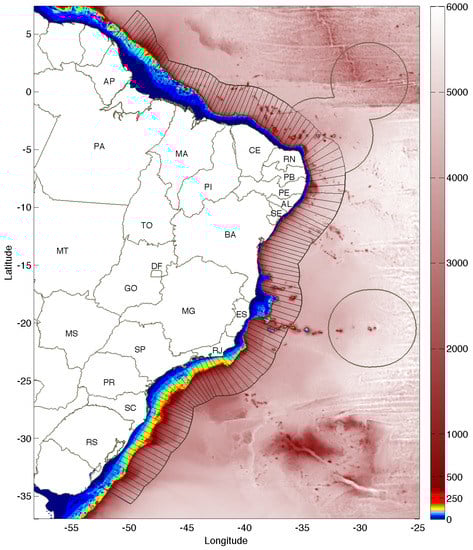
Figure 1.
Study region’s bathymetry and Brazilian states. ETOPO1 depth (see Amante et al. 2009; [31]) is depicted by a color shade in meters. The thick gray line corresponds to the Exclusive Economic Zone (EEZ), while thin gray lines represent the coastal sectors defined for data processing and visualization. Coastal states are: Amapá (AP), Pará (PA), Maranhão (MA), Piauí (PI), Ceará (CE), Rio Grande do Norte (RN), Paraíba (PB), Pernambuco (PE), Alagoas (AL), Sergipe (SE), Bahía (BA), Espírito Santo (ES), Rio de Janeiro (RJ), São Paulo (SP), Paraná (PR), Santa Catarina (SC) and Rio Grande do Sul (RS).
2.4. Wind Data Vertical Extrapolation
Satellite data provide observations near the surface at z = 10 m height, so vertical extrapolation is necessary to assess wind speeds at the height of modern wind turbines.
Under neutral conditions, the wind profile is controlled by friction and usually modeled by a logarithmic law [33]. More often, turbulent exchanges of heat between the ocean and the atmosphere will modify the atmospheric stability. Convection (unstable condition) occurs whenever the heat flows from the ocean to the atmosphere (i.e., atmosphere heated by the ocean). On the other hand, stable (stratified) conditions tend to occur when the heat flux is from the atmosphere to the ocean (i.e., ocean cooling the atmosphere). The convention adopted here is that positive (negative) fluxes indicate heat towards the atmosphere (ocean).
The Monin–Obukhov similarity theory provides a semi-empirical framework to model the boundary layer under the effects of momentum and buoyancy exchanges [25]. Here we follow the method of Capps and Zender [26], employing a wind product that has a larger time coverage (∼26 years) and better temporal resolution (6 h).
According to the theory the wind speed dependence on height z can be modeled by:
where z is the height above the ocean surface and is the von Karman constant. Friction velocity is a function of the satellite wind speed U at 10 m height and a neutral drag coefficient [27,39]. The parameter is the roughness length, and is an empirically derived stability function. L is the Monin–Obukhov length scale (m):
is the virtual potential temperature: = (1 + 0.6087 ), with as the specific humidity (kg kg) and as the potential temperature: = (10/P), where P is the surface pressure (Pa) and is the surface air temperature (K) [25]. is the buoyancy flux and is the virtual potential temperature flux [26,40]. The latter depends on the exchanges of specific and latent heat fluxes (W m) [26]:
The specific heat is 1004.67 (J·kg·K), the air density (kg·m) and (J·kg) is the latent heat of vaporization. Air density is = ), with R = 287.04 as the specific gas constant (J·kg·K) and as the virtual temperature = . Latent heat is = 2.45 × (J·kg).
With the Monin–Obukhov length scale, one can estimate the stability function from empirical relationships [26,41]. Under unstable conditions ():
where . For slightly stable cases (0 < < 0.5):
And finally, for very stable conditions ( ≥ 0.5) [26,42]:
Please note that for neutral cases ∼0 so that Equation (3) reduces to the so-called logarithmic wind profile [33]:
A hub height of z = 95 m, compatible with modern wind turbines is considered for all computations. A constant roughness parameter = 0.2 mm will be considered when extrapolating wind speeds considering neutral atmosphere conditions (Equation (9)), as in previous works [13,19].
Whenever winds are vertically extrapolated accounting for atmospheric stability (Equation (3)), Charnock’s relation for aerodynamic roughness, will be employed. Here , typical of open-ocean conditions. Charnock’s hypothesis assume that winds are blowing steadily and long enough for the wave field to be in complete equilibrium with the wind field, independent of fetch [25]. These conditions might be limited near the coast, particularly in situations when the wind blows from the shore. Extrapolated wind fields will be referred as for neutral conditions (hereafter referred as log-law method) and when accounting for atmospheric stability (Monin–Obukhov or stability-based method).
2.5. Wind Power and Resource Integration
In this work we selected five wind turbines designed for marine installations. Vestas V112-3.3 MW (hereafter VE 3.3), General Electric 3.6s Offshore (GE 3.6), Siemens SWT-3.6-120 (SI 3.6), Senvion 6.2M 152 (SE 6.2) and Vestas V164-8.0 MW (VE 8.0). These horizontal axis turbines are composed of three blades with diameters that vary from 104 to 164 m and swept areas that range from 8495 to 21,124 m (Table 1).

Table 1.
Modern wind turbine characteristics. Vestas V112-3.3 MW (VE 3.3), General Electric 3.6s Offshore (GE 3.6), Siemens SWT-3.6-120 (SI 3.6), Senvion 6.2M 152 (SE 6.2) and the Vestas V164-8.0 MW (VE 8.0).
Empirically derived power curves are provided by turbine manufacturers and are shown in Figure 2. Turbines start to produce power with speeds around 3.0 m·s, referred to as the “cut-in” speed. After that, the power generation grows proportionally to the cube of wind magnitude, until the turbine reaches its maximum capacity. Beyond the “rated speed” the turbine generates constant output until the “cut-out” speed is reached. That refers to the wind magnitude at which the turbine shuts down for self-protection (Table 1).
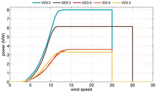
Figure 2.
Empirically derived power curves for Vestas V112-3.3 MW (hereafter VE 3.3), General Electric 3.6 s Offshore (GE 3.6), Siemens SWT-3.6-120 (SI 3.6), Senvion 6.2 M 152 (SE 6.2) and the Vestas V164-8.0 MW (VE 8.0).
These curves establish a functional relation of wind speeds to power production , and will be used for the technical assessment. The log-law and Monin–Obukhov power estimates will be respectively referred to as and , using wind speeds obtained by these two methods (see Equations (3) and (9)).
As power curves assume a reference air density of 1.225 kg·m that is typical of temperate regions (15 C and 1 atm), one further adjustment can be made to account for the temporal and latitudinal variability of air density (see Lu et al. 2009, [43]). An adjusted wind speed can be estimated from:
where is the wind speed estimated from the stability-based method, is the air density at the hub height, estimated from the thermodynamic database, and refers to the “corrected” wind speed. Hereafter we will refer to as the estimate that takes into account both the atmospheric stability and the air density distribution.
The resource estimation can be finally calculated from:
Here n refers to the number of grid points considered for a specific area, is the time-averaged turbine power (either , , or ), and (km) is the area of the grid point with index i. is the number of turbines installed per km, assuming a spacing of 10 rotor diameters downwind and 5 crosswind [19,33]. This corresponds, for example, to = 0.54 km per GE 3.6 turbine and 0.62 km per VE 8.0 turbine (Table 1). As the bathymetric data from ETOPO1 have higher spatial resolution (∼0.016) than fields (0.25), the latter was interpolated to the higher resolution grid, thus better representing the power distribution for practical bathymetric intervals.
3. Results
3.1. Air, Sea Surface Temperature and Heat Fluxes
Figure 3 illustrates the along-coast variability of selected thermodynamic variables, while Figure 1 provides the geographical reference. The x-axis in Figure 3 represents the distance along the coast, from its northern limit at Amapá (0 km) to its southern end at the international border of Rio Grande do Sul state (7000 km). Graphs were obtained by averaging the climatological information for the sectors defined by Figure 1 and considering the data between 0 and 100 m depth. State symbols are indicated in the bottom panel.
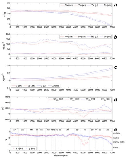
Figure 3.
Along-coast variability of thermodynamic fields. Here the x-axis represents the distance (km) along the Brazilian coast, from its northern limit at Amapá (AP, left) to its southern end at Rio Grande do Sul (RS, right). (a) air () and sea surface () temperatures. (b) sensible () and latent () heat fluxes. (c) surface () and hub-height () air densities. (d) surface virtual temperature fluxes due to sensible () and latent heats (). (e) dimensionless stability function . Colors refer to January (red) and July (blue). All quantities were averaged along the sectors shown in Figure 1 up to depths of 100 m. Coastal states’ labels are shown in the bottom panel.
Surface atmospheric () and sea surface temperatures () for January and July are shown in Figure 3a. The northern and northeastern shelves are under direct influence of the warm and salty tropical waters of the North Brazil and Brazil currents [44,45]. Seasonal variability is small and and are around 27 ± 1C in this region. Towards the poles, and decrease, also presenting substantial seasonal variability. Southern temperatures are around 24 C in January and 15 C in July.
Sea surface temperature is generally 1 to 2 C warmer than the air temperatures for most of the coastal extent, with some exceptions. During the summer, RJ and ES coasts (∼5000 km) present colder waters than the atmosphere ( < ) due to the phenomenon of coastal upwelling. Cold waters are upwelled to the surface due to the predominant offshore transport of surface waters [46,47]. In the north and northeast, ocean temperatures tend to be slightly larger than atmospheric temperatures () bordering AP to BA coasts. During the winter, on the other hand, prevailing southern winds promote the coastal intrusion of relatively cold and fresh waters associate to Plata river plume, causing a drop of temperatures along RS, SC, PR and SP coasts [48,49,50,51]. Although in average terms the ocean is warmer than the atmosphere in these regions, cold-water intrusions can generate situations where .
Average heat fluxes are shown in Figure 3b. Positive (negative) fluxes indicate heat flow towards the atmosphere (ocean). Latent heat flux () is predominantly positive, around 50 to 150 W m, with fluxes in July generally larger than January. Sensible heat () is generally positive around 10 to 20 W m, but with exceptions. fluxes are close to zero along MA and PI and negative for RJ coast, indicating a mean flow towards the ocean.
Air density is inversely related to air surface temperature, as illustrated in Figure 3c. Surface () and hub-height () densities are plotted for the months of January and July. Lower densities of 1.15 kg·m are observed in the north, increasing to 1.21 ± 0.03 in the south. Height decay is small, around 0.01 kg·m. According to Equation (10), the largest density ratios are on the order of 0.94, so velocity corrections can be as large as .
Surface fluxes are show in Figure 3d. The first term of the right-hand side of Equation (5) is the contribution from sensible heat. This quantity is shown by a continuous line on this graph and by the symbol . During the austral summer is generally positive, except for ES and RJ coast where < 0, due to coastal upwelling. During the austral winter values are positive or fairly small for the coast of MA and PI. The second term of the right-hand side of Equation (5), the latent heat contribution , is shown by a dashed line. Its climatological average is generally positive along the coast in both seasons.
3.2. Surface Layer Stability
The stability function distributions for January and July are shown on the map of Figure 4. Here is estimated from Equations (4) to (8) using OAFLUX, NCEP and BSW datasets for the period of 1987–2014. According to these definitions, stable and slightly stable atmospheric conditions are indicated respectively by and −2.5 ≤ < 0, or blue colors. Near neutral situations ∼ 0 are shown in white and unstable conditions > 0 are denoted by red tones.
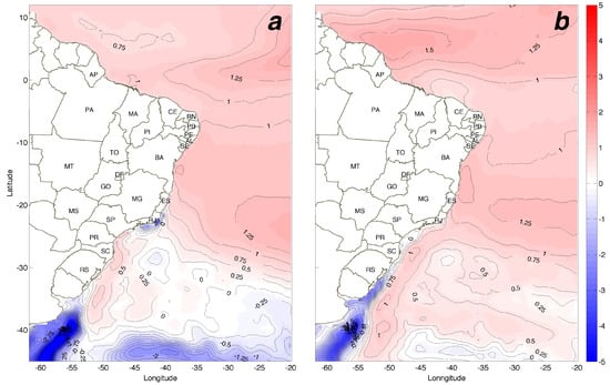
Figure 4.
Surface layer dimensionless stability function for (a) January and (b) July. is computed from thermodynamic properties derived from OAFLUX, NCEP and BSW datasets (1987–2014). Intervals are: stable atmospheric conditions ( < −2.5), slightly stable (−2.5 ≤ < 0), neutral ( ∼ 0) and unstable conditions ( > 0).
The tropical waters of the north and northeast coasts are characterized by positive heat and buoyancy fluxes, so the predominant part of Brazil’s coastal zone is characterized by unstable conditions. This is also reflected in Figure 3e, which illustrates along-coast distribution. is generally positive and hardly changes from summer to winter between PA and BA indicating unstable conditions. Southeast and south coasts are an exception and present situations that vary from neutral to slightly stable conditions near the coast. In the austral summer, there is upwelling of cold waters between Cabo São Tomé (ES) and Cabo Frio (RJ) (see Figure 2 of Rodrigues and Lorenzzetti [46] and Figure 4 of Palóczy et al. [47]). This tends to stratify the lower atmosphere in this region so that (Figure 3e and Figure 4a).
During the austral winter, neutral to slightly stable conditions dominate the coasts of Uruguay and RS to SP states due to the northern advection of colder waters driven by southwesterly winds [49,50,51,52,53]. The blue shaded area shown in Figure 4b reminds the average position of the Rio de la Plata plume intrusion (see Figure 1 of Campos et al., 1996 [54] and Figure 3 of Möller et al., 2008 [50]). Further south, offshore of Mar del Plata, Subantarctic waters carried by the Malvinas currents generate stable atmospheric conditions ( < −2.5) in the summer and winter. The eastward change of from stable to unstable conditions that occurs around 57 W is coincident with the position of the Brazil–Malvinas confluence [45,55].
3.3. Wind Speed Distributions
Climatological (1987–2014) wind fields for January and July are respectively shown in Figure 5. Here the colors indicate the wind speed at the hub height (z = 95 m) estimated with the stability-based method (see Equation (3)). Wind direction is depicted by streamlines.
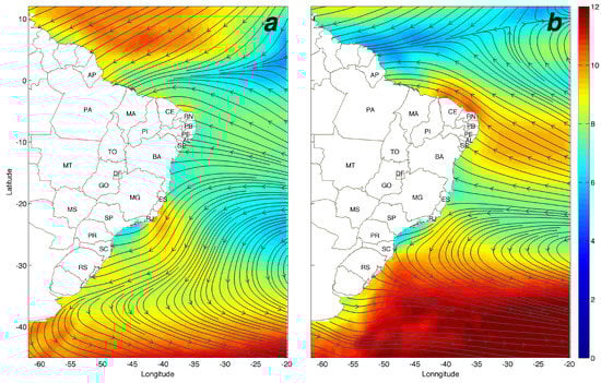
Figure 5.
Climatological (1987–2014) wind speeds and streamlines for (a) January and (b) July. Colors indicate wind speed at hub height. Winds were extrapolated to z = 95 m using the Monin–Obukhov stability-based method. States’ names are indicated in Figure 1.
Dominant features are the Trade Winds and Intertropical Convergence Zone (ITCZ), the Westerlies and the presence of the South Atlantic Subtropical High, also referred as the South Atlantic Anticyclone (SAA). The ITCZ is identified by a zonal stretch of low horizontal wind speeds (doldrums) that migrates from 0 in January (Figure 5a) to 5 N in July (Figure 5b). With the ITCZ southward position, northeast trades generate strong 8.5 m·s winds at the AP and PA coasts in January. The southeast trades create even stronger winds at the coasts of PB, RN, CE, PI and MA in July (∼10 m·s), when the ITCZ migrates northward (Figure 5b).
The SAA is located near 30 S and 20 W in January, when northeasterly to easterly mean winds dominate the southeastern and southern Brazilian coasts. Northeast winds are especially strong over RJ (9 m·s), SC and RS (8.5 m·s). In July the SAA migrates northward to 28 S and the Westerlies become more dominant for RS coast. Brazil’s southern region experiences synoptic changes of wind conditions. Cold fronts hit the area frequently throughout the year, but with more force in the fall-winter [56,57]. Average July wind speeds are around 10 m·s on SC, RS, and RN, and CE coasts.
3.4. Atmospheric Stability Impact on Wind Estimations
Hub-height wind magnitudes estimated with the stability-based method are different from the wind fields obtained for a neutral atmosphere [13,19,58,59,60]. Here their difference is shown in Figure 6, where colors depict , where is the stability-based speed and the neutral atmosphere (log-law) estimate. As shown by the blue tones, over most of the continental shelf the log-law can overestimate winds from 0.5 to 1 m·s. For a few locations the classical method (log-law), can underestimate winds. During the summer winds can be underestimated at RJ and ES coasts. Likewise, winds tend to be underestimated on RS coast during the winter. The maps of Figure 6 illustrate that the stability-based method predicts stronger wind speeds in these locations.
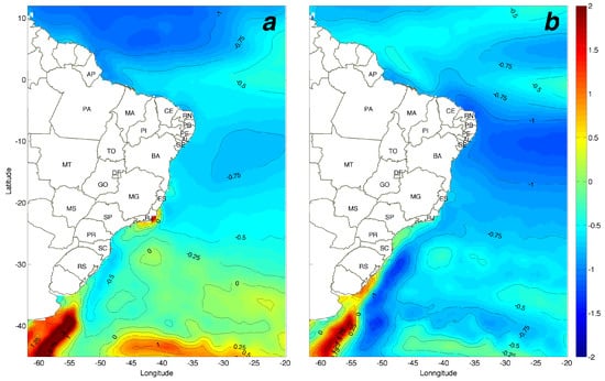
Figure 6.
Hub-height wind speed field differences () for (a) January and (b) July, comparing the effect of atmospheric stability on winds vertical extrapolation. and refer to the winds extrapolated with the stability-based (Monin–Obukhov) and log-law methods, respectively. Contours and colors indicate the speed in m·s. States names are listed in the legend of Figure 1.
These wind estimates can be further compared by Figure 7a,b along-coast distributions. January wind speeds at z = 10 m height are indicated by a black line and vary from 5 to 9 m·s with faster winds observed for AP, PA, MA, PI, CE, RN, ES, RJ, SC and RS states. The log-law wind estimate (blue line) predicts an average vertical shear (difference to 10 m winds) of about 2 m·s throughout the study region, while the stability-based method (red) mean vertical shear is around 1 m·s for most of the coast, but can reach up to 3 m·s for the RJ coast. The density corrected wind speed (orange line) estimated from Equation (10) slightly reduces the speed. In July wind speeds increase for PI, CE, RN states, with 10 m·s computed from the stability-based method . Differences among the extrapolation methods are relatively the same as observed for January for most of the country extent. An exception occurs in July for the southeast SP, PR and southern SC, RS states when differences among the methods are small, as atmospheric conditions tends to neutral. For the southern end of RS state, conditions in July demonstrate that > .
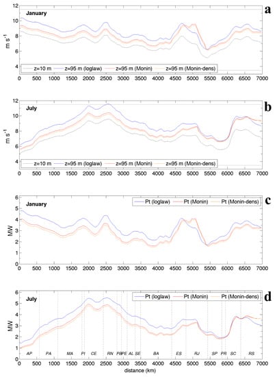
Figure 7.
Along-coast variability of wind speed and turbine power. The x-axis represents the distance (km) along the Brazilian coast, from its northern limit at Amapá (AP, left) to its southern end at Rio Grande do Sul (RS, right). Panels (a,b) are wind magnitudes at z = 10 m and at the hub height (z = 95 m), computed with three different methods for January and July, respectively. Panels (c,d) are power distributions estimated from SE 6.2 power curve and three methods for January and July, respectively. Labels refer to the logarithmic extrapolation method (log-law, ), the Monin–Obukhov (Monin, ) and Monin–Obukhov with density correction (Monin-dens, ). All quantities were averaged along the sectors shown in Figure 1 up to depths of 100 m. States names are listed in the legend of Figure 1.
3.5. Turbine Power Fields
Turbine power fields for January and July are respectively shown in Figure 8. Colors indicate the generated power simulated with the Senvion SE6.2 wind power curve (Table 1), considering the stability-based method and the density correction procedure. January resources are large for AP, PA, PI, CE, RN, ES, RJ, SC and RS coasts with > 3.0 MW, a capacity factor (CF) of 48%. During this season, winds are weak off SP and PR and also for the northeast, from PB to BA.
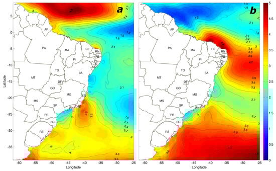
Figure 8.
Climatological (1987–2014) turbine power for (a) January and (b) July for the height of z = 95 m, considering the Monin–Obukhov extrapolation method, the correction for air density and the SE 6.2 turbine power curve (see Section 2.5).
In July, the trade winds intensify over the northeast at MA, PI, CE, RN, PB, PE and AL states with > 3.0 MW. Peak power of 4.2 MW (CF ∼67%) are observed to RN and CE coasts. Winter winds generate an average > 3.6 MW for SC and RS (CF ∼58%). During this time of year, power production decays for AP and remains low for BA, northern ES, southern RJ, SP and PR states.
Figure 7c,d compares the power estimated from winds calculated with the three methods of extrapolation. It becomes clear how the log-law overestimates January power by nearly 1 MW for a 5000 km stretch of coastline between AP and ES. It also demonstrates the importance of the stability-based method to extrapolate winds for RJ coast. During the summer the log-law underestimate the power generation in this region, which is 1 MW higher when computed with the stability-based method (Figure 7c). In July the log-law overestimates power by 0.5 MW from AP to ES. Differences are small for the states of SP, PR and SC, but the relatively stable atmospheric conditions found in RS can lead to underestimation of 0.5 MW by the log-law method (Figure 7d).
3.6. Seasonal Variability
A more complete picture of the monthly evolution of power along the coast is reproduced in Figure 9. Here we plot the average output obtained with the Senvion SE6.2 power curve, considering the stability-based method with the density correction procedure (Equation (10)).
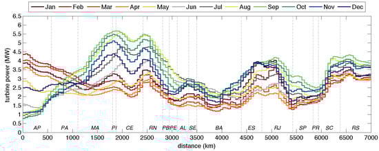
Figure 9.
Turbine power distribution along the Brazilian coast, from Amapá (AP) in the north to Rio Grande do Sul (RS) on the southern border. Colored lines represent the monthly climatological (1987–2014) power for a Senvion 6.2 turbine. The Monin–Obukhov extrapolation method and the density correction of Equation (10) are considered.
The curves evidence windy regions off Brazil’s coastline for the states of Amapá (AP), Pará (PA), Maranhão (MA), Piauí (PI), Ceará (CE), Rio Grande do Norte (RN), Paraíba (PB), Pernambuco (PE), Espírito Santo (ES), Rio de Janeiro (RJ), Santa Catarina (SC) and Rio Grande do Sul (RS). Production generally peaks from the late winter (Aug) through spring (Sep, Oct, Nov). The exception is the AP coast, which has low production during these months. September is the peak production for PI, CE and RN coasts reaching 5.5 MW (CF of 89%). Strong winds are also found for ES and RJ (4 MW) and the southern states of SC and RS (4.5 MW) for the same period.
The lowest production for most of the coastline is observed in summer (Dec, Jan, Feb) and fall (Mar, Apr, May). Production can fall to 3 MW in March for PI, CE and RN coasts, 2.5 MW for ES, RJ and 3.0 MW for SC and RS. But surprisingly, production peaks in March for the coasts of AP and PA, reaching from 3 to 4.5 MW per SE6.2 turbine (CF of 48 to 72%). This seasonal seesaw pattern is associated with the migration of the ITCZ: whenever the ICTZ migrates south, northeast trades increase the power production for AP and PA, with the doldrums near MA, PI and CE. When the ITCZ migrates north, southeast trades intensify over PI, CE, RN and PB coasts, and wind decay is observed off AP coast (see Figure 8 and Figure 9).
3.7. Resource Distribution
The wind resource is not only dependent on site-specific average power, but also on the local area available for placing wind turbines. Moreover, marine installation of wind turbines is dependent on depth. Present bottom-mounted technology allows exploitation up to 60 m [6]. The most widely adopted foundation systems of Europe are monopiles (80%), followed by gravity foundations (9.1%), jacket structures (5.4%), tripods and tripiles (5.3%) [61]. It is anticipated that floating structures, in the demonstration stage, will soon be commercially available for depths between 50 and 100 m [5,6,7,8]. Here the resources were evaluated for existing and future technologies according to specific depth intervals, as explained below.
Bathymetry from ETOPO1 and turbine average power were combined through Equation (11) to find the wind resource over particular ocean regions. Area integration was performed considering the 1984 World Geodetic System (WGS 84). Power production was computed from vertically extrapolated satellite data and the turbine characteristics of Table 1 and Figure 2.
Figure 10 summarizes the results for shelf area, turbine mean power and resource distribution R. The y-axis represents the distance along the coastline, from north Brazil at Amapá (AP, top) to the south at Rio Grande do Sul state (RS, bottom). Area and resource distributions shown were integrated inside of the 136 sectors indicated in Figure 1, while the power distribution was averaged over these areas. Sectors’ coastal widths vary from 50 to 53 km and state symbols are shown on the right axis.
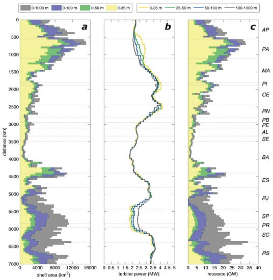
Figure 10.
(a) Shelf area, (b) turbine mean power and (c) resource distribution R. Here the y-axis represents the distance (km) along the Brazilian coast, from its northern limit at Amapá (AP, top) to its southern end at Rio Grande do Sul (RS, bottom). Shelf area (km) is computed from ETOPO1 data using the section divisions of Figure 1. Filled curves correspond to depths intervals that vary from 0–35 m (yellow) to 0–1000 m (gray). Turbine average power is computed for the depth intervals: 0–35 m, 35–50, 50–100 and 100–1000 m. Wind resource (GW) is estimated from for the same depth intervals used in the area computation (panel a). Estimates are based on the SE 6.2 power curve, considering Monin–Obukhov vertical extrapolation and the density correction of Equation (10). Coastal states’ divisions are depicted by horizontal dashed lines and their labels are placed on the right.
Northern states of AP, PA and MA stand out with their broad and shallow continental shelves (Figure 10a). This region corresponds to nearly 155,924 km or 48.9% of the country’s shelf between 0 and 35 m depth (318,618 km). Vitória-Trindade chain peaks on the shelf area distribution off BA and ES coasts (13.3 % in area). The broad shelf of RS state has 21,034 km or 6.6% of the area between 0 and 35 m. If extending the depth range to 100 m, the main areas are on the north (AP to MA, 258,954 km) and southeast and south (RJ to RS, 178,741 km). These regions correspond respectively to 44% and 30% of the country’s area for this depth range (589.465 km ).
Average power distribution of Figure 10b resembles the wind distribution of Figure 9, but here the turbine mean power variability with depth is explored. Interestingly, turbine mean power is larger in shallower depths over the north and northeast. This is particularly true for PA, where the average power increases from 2.2 MW in deeper waters (100–1000 m) to 2.8 MW in shallower waters (0–35 m). Similar distributions are observed for PI, CE and RN, even though their shelves are much narrower. For SP and PR, the South Brazil Bight, the reverse is observed. Mean turbine power increase with the distance offshore, varying from 1.9 MW (0–35 m) to 2.4 MW offshore. For SC there is a slight increase of power offshore and for RS no significant change is observed across the shelf.
Technical resource is plotted in Figure 10c. Large resources (369 GW) are found for AP, PA and MA between 0 and 35 m depth. This is nearly 50.6% of the total country resources (729 GW) for this depth interval. Other states with good resources are CE (86.7 GW, 12%), RN (34.9 GW, ), SP (22.5 GW, 3%) and RS (59.5 GW, 8.2%).
When the depth limit is increased to 100 m, resources between AP, PA and MA increase to 592 GW, or 43.9% of the country’s resource (1346 GW). The estimated resource for RS and SC is 245 GW (18.2 %) between 0 and 100 m, which is larger than estimated by Pimenta et al., (2008) (217 GW) for a similar shelf area [13]. Resources for the same region between 0 and 50 m are 115 GW.
The country’s integrated quantities are shown in Table 2, which further highlights results for different methods of extrapolation and wind turbines. Here refers to the power computed from log-law extrapolation. refers to the stability-based method (Monin–Obukhov) and as the combination of the stability method with the density correction procedure.
Table 2.
Wind resource potential R (GW) as function of depth interval and wind turbine. Numbers refer to the average resource estimated from turbine power estimates: Monin–Obukhov (), Monin–Obukhov and density correction () and the log-law () methods.
Overall, there is a 10 to 20% decay of the country’s wind resource when considering the stability-based method and another 5% decay when considering the density correction routine. Estimates usually vary within 2% for different turbine technologies, but sometimes can differ by 23%. The best performances were observed for SE 6.2 and VE 8.0 turbines (Table 2).
Accounting for atmospheric instability and the air density, offshore resources between 0–35 m are around 725 GW, increasing to 980 GW between 0–50 m depth and around 1.3 TW for 0–100 m range. Considering the EEZ contiguous to the Brazilian coast, the technical potential is 7.2 TW. The Trindade EEZ region alone has a resource of 880 GW. These estimates do not consider exclusion zones, such as marine conservation areas, shipping lanes, commercial fishing or oil exploration regions. Studies suggest that exclusion areas should reduce resources by 10 to 46% [62].
4. Summary and Conclusions
Brazil’s offshore wind resources were estimated from historical datasets (1987–2014). Satellite information derived from BSW product provided wind speeds at 10 m height at 0.25 spatial and 6 h temporal resolution. Climatological data derived from OAFLUX provided air and sea temperatures, specific humidity, latent and sensible heat fluxes. A stability-based method was used to estimate winds at the hub height of wind turbines, taking into account the space-time variability of atmospheric and oceanic conditions. Technical data and the power curves of five modern wind turbines were used to estimate the site-specific generated power. Results were combined with bathymetric data for integration of power resources according to different depth intervals.
Oceanographic and atmospheric conditions vary substantially along Brazil’s coastal margin, impacting the atmospheric stability and the wind power potential. In the north and northeast (5 N–18 S), warm tropical waters tend to create unstable atmospheric conditions and weak vertical wind shear. As a result, when extrapolating winds to the height of turbines, the stability-based estimates () are 0.5 to 0.75 m·s lower than those obtained with the traditional log-law (), which considers a neutral atmosphere.
Neutral to unstable conditions are observed in January for the southeast and southern coasts (22 S–33 S), with exception for Cabo Frio upwelling where slightly stable atmospheric conditions prevail. For this reason, winds estimated by the stability-based method will be 0.5 to 2 m·s higher than winds estimated by the traditional log-law for Rio de Janeiro (RJ) shelf. In regions with neutral atmospheric conditions there is little difference between the wind speeds extrapolated with these two methods.
During the austral winter, the southeastern and southern coasts experience neutral to slightly stable conditions due to the southern intrusion of cold waters associated with Plata plume. Vertical shears predicted with the stability-based method are therefore equal or larger than predicted by the traditional log-law. The stability-based method predicts winds up to 0.5 m·s stronger than previous estimates.
Attractive hotspots occur along Brazil’s continental margin, for initial offshore wind development. Strong winds are present off the north states (AP, PA) states with mean turbine power and capacity factors (CF) that vary from 4.5 MW (72% CF) in February to 3.5 MW (56% CF) in September (Estimates correspond to SE6.2 power curve per Figure 9). For northeast states of MA, PI, CE, RN mean turbine power and capacity factors vary from 3.0 MW (48% CF) in February to 5.5 MW (88% CF) in September. Other attractive locations are the southeast states of ES and RJ, with mean power varying from 2.5 MW (40% CF) in March to near 4.5 MW (72% CF) in September. Southern states of SC and RS have mean power that varies from 3.0 MW in March (48% CF) to 4.2 MW (67% CF) in September.
A seesaw seasonal variability was observed between the north and northeast regions (Figure 9). This occurs due to the migration of the ITCZ and intensification of the South Atlantic Subtropical High pressure. This type of regional complementarity was also observed in previous works [19,60]. Development of multi-connected wind farms (super-grids) [1,9] could be considered to reduce power fluctuations and for seasonal balancing of future northern and northeastern wind farms. Offshore winds are complementary to hydrological resources and should help on the management of Brazil’s large hydroelectric reservoirs [19,63].
Brazil’s offshore wind resources are significant. When accounting for modern technology and atmospheric surface layer stability, we found around 725 GW between 0–35 m, 980 GW for 0–50 m, 1.3 TW for 0–100 m and 7.2 TW for the ocean region delimited by the contiguous Exclusive Economic Zone. Resources add up to 8.0 TW when the EEZ around Trindade and Martin Vaz Archipelago are included.
Results described in this article should be used with caution as they still need to be compared with tower observations. Satellite winds from SAR and model atmospheric downscaling should help on the description of orographic effects for winds near the coast that are not resolved by the BSW satellite product.
Future studies will clearly depend on multiple observations along Brazil’s continental shelf. The installation of meteorological towers combined with the use of LIDAR technology mounted over buoys and ships should be a necessary step to improve the knowledge of Brazilian sea winds.
Author Contributions
F.M.P.—conceptualization, formal analysis, methodology, software, writing, review and editing. A.R.S.—methodology, software, writing, review and editing. A.T.A., V.d.S.e.A. and O.R.S.—formal analysis, writing, review and editing. The final manuscript has been approved by all authors.
Funding
This research was funded by FAPERN grant number (005/2011), CAPES, CNPq grant numbers (406801/2013-4, 465672/2014-0, 311930/2016-6, 309315/2015-8) and FAPEMIG (APQ 01575-14).
Acknowledgments
F.M.P. acknowledges FAPERN (005/2011), CAPES and CNPq (406801/2013-4, 465672/2014-0, 311930/2016-6) for financial support. A.T.A. acknowledges the support of FAPEMIG (APQ 01575-14), CAPES and CNPq (465672/2014-0, 309315/2015-8). The original manuscript was improved through the helpful comments of three anonymous reviewers.
Conflicts of Interest
The authors declare no conflict of interest.
References
- Rodrigues, S.; Restrepo, C.; Kontos, E.; Pinto, R.T.; Bauer, P. Trends of offshore wind projects. Renew. Sustain. Energy Rev. 2015, 49, 1114–1135. [Google Scholar] [CrossRef]
- Wind Europe. Offshore Wind in Europe. Key Trends and Statistics 2018; Technical Report; Wind Europe: Brussels, Belgium, 2018; Available online: https://windeurope.org (accessed on 14 April 2019).
- GWEC. Global Wind 2018 Report; Technical Report; Global Wind Energy Council: Brussels, Belgium, 2018; Available online: http://www.gwec.net (accessed on 14 April 2019).
- Wind Europe. Wind Energy in Europe: Scenarios for 2030; Technical Report; Wind Europe: Brussels, Belgium, 2017; Available online: https://windeurope.org (accessed on 14 April 2019).
- Musial, W.; Butterfield, S.; Ram, B. Energy from Offshore Wind; Technical Report; NREL/CP-500-39450; National Renewable Energy Laboratory (NREL): Golden, CO, USA, 2006. [Google Scholar]
- Arshad, M.; O’Kelly, B.C. Offshore wind-turbine structures: A review. Proc. ICE-Energy 2013, 166, 139–152. [Google Scholar] [CrossRef]
- Hywind. Building the World’s First Floating Offshore Wind Farm; Technical Report; Hywind, Statoil: Grampian, UK, 2015; Available online: http://www.statoil.com (accessed on 28 February 2018).
- Hywind. Hywind Scotland Pilot Park; Technical Report; Hywind, Statoil: Grampian, UK, 2016; Available online: http://www.statoil.com (accessed on 27 April 2018).
- Kempton, W.; Pimenta, F.M.; Veron, D.E.; Colle, B.A. Electric power from offshore wind via synoptic-scale interconnection. Proc. Natl. Acad. Sci. USA 2011, 107, 7240–7245. [Google Scholar] [CrossRef]
- Decker, J.D.; Woyte, A. Review of the various proposals for the European offshore grid. Renew. Energy 2013, 49, 58–62. [Google Scholar] [CrossRef]
- Storrer, M.; Garcia, P.; Barbosa, E.E. The Asa Branca offshore wind farm—A change for the creation of a new cluster for the supply of 10 GW of multimegawatt wind turbines in Brazil. In Proceedings of the European Offshore Wind Conference and Exhibition, Stockholm, Sweden, 14–16 September 2009; Wind Europe: Stockholm, Sweden, 2009. [Google Scholar]
- Tenproject. Offshore Wind Energy—Progettazione, studi di fattibilita e studi paesaggistici; Technical Report; Ten Project: San Giorgio del Sannio, Italy, 2015; Available online: https://www.tenproject.it/eolico-offshore (accessed on 27 March 2019).
- Pimenta, F.M.; Kempton, W.; Garvine, R.W. Combining meteorological stations and satellite data to evaluate the offshore wind power resource of Southeastern Brazil. Renew. Energy 2008, 33, 2375–2387. [Google Scholar] [CrossRef]
- Liu, W.T.; Tang, W.; Xie, X. Wind power distribution over the ocean. Geophys. Res. Lett. 2008, 35, L13808. [Google Scholar] [CrossRef]
- Capps, S.B.; Zender, C.S. Estimated global ocean wind power potential from QuikSCAT observations, accounting for turbine characteristics and siting. J. Geophys. Res. 2010, 115. [Google Scholar] [CrossRef]
- Hasager, C.B. Offshore winds mapped from satellite remote sensing. WIREs Energy Environ. 2014, 3, 594–603. [Google Scholar] [CrossRef]
- Hasager, C.B.; Mouche, A.; Badger, M.; Bingol, F.; Karagali, J.; Driesenaar, T.; Stoffelen, A.; Peña, A.; Longépé, N. Offshore wind climatology based on synergetic use of Envisat ASAR, ASCAT and QuikSCAT. Remote Sens. Environ. 2015, 156, 247–263. [Google Scholar] [CrossRef]
- Doubrawa, P.; Barthelmie, R.J.; Pryor, S.C.; Hasager, C.B.; Badger, M.; Karagali, I. Satellite winds as a tool for offshore wind resource assessment: The Great Lakes Wind Atlas. Remote Sens. Environ. 2015, 168, 349–359. [Google Scholar] [CrossRef]
- Silva, A.R.; Pimenta, F.M.; Assireu, A.T.; Spyrides, M.H.C. Complementarity of Brazil’s hydro and offshore wind power. Renew. Sustain. Energy Rev. 2016, 56, 413–427. [Google Scholar] [CrossRef]
- Karagali, I. Scatterometry for wind energy. In Remote Sensing for Wind Energy; Report-0029 (EN); Pena, A., Karagali, I., Eds.; DTU Wind Energy, Riso Campus: Roskilde, Denmark, 2013; pp. 296–308. [Google Scholar]
- Lange, B.; Larsen, S.; Hojstrup, J.; Barthelmie, R. Importance of thermal effects and sea surface roughness for offshore wind resource assessment. J. Wind Eng. Ind. Aerod. 2004, 92, 959–988. [Google Scholar] [CrossRef]
- Barthelmie, R.J. The effects of atmospheric stability on coastal wind climates. Met. Appl. 1999, 6, 39–47. [Google Scholar] [CrossRef]
- Sathe, A.; Gryning, S.E.; Peña, A. Comparison of the atmospheric stability and wind profiles at two wind farm sites over a long marine fetch in the North Sea. Wind Energy 2011, 14, 767–780. [Google Scholar] [CrossRef]
- Archer, C.L.; Colle, B.A.; Veron, D.L.; Veron, F.; Sienkiewicz, M.J. On the predominance of unstable atmospheric conditions in the marine boundary layer offshore of the U.S. northeastern coast. J. Geophys. Res. 2016, 121, 8869–8885. [Google Scholar] [CrossRef]
- Arya, S.P. Introduction to Micrometeorology; International Geophysics Series; Academic Press: San Diego, CA, USA, 2001; p. 420. [Google Scholar]
- Capps, S.B.; Zender, C.S. Global ocean wind power sensitivity to surface layer stability. Geophys. Res. Lett. 2009, 36. [Google Scholar] [CrossRef]
- Thomas, N.; Seim, H.; Haines, S. An Observational, Spatially Explicit, Stability-Based Estimate of the Wind Resource off the Shore of North Carolina. J. Appl. Meteorol. Climatol. 2015, 54, 2407–2425. [Google Scholar] [CrossRef]
- Badger, M.; Peña, A.; Hahmann, A.N.; Mouche, A.A.; Hasager, C.B. Extrapolating Satellite Winds to Turbine Operating Heights. J. Appl. Meteorol. Climatol. 2016, 55, 975–991. [Google Scholar] [CrossRef]
- Yu, L.; Weller, R.A. Multidecade Global Flux Datasets from the Objectively Analyzed Air-Sea Fluxes (OafLux) Project: Latent and Sensible Fluxes, Ocean Evaporation, and Related Surface Meteorological Variables; Technical Report; OA-2008-01; WHOI, Woods Hole Oceanographic Institute: Woods Hole, MA, USA, 2008. [Google Scholar]
- Kanamitsu, M.; Ebisuzaki, W.; Woollen, J.; Yang, S.K.; Hnilo, J.J.; Fiorino, M.; Potter, G.L. NCEP-DOE AMIP-II Reanalysis (R-2). Bull. Am. Meteorol. Soc. 2002, 1631–1643. [Google Scholar] [CrossRef]
- Amante, C.; Eakins, B. ETOPO1 1 Arc-Minute Global Relief Model: Procedures, Data Sources and Analysis; Technical Memorandum NESDIS NGDC-24; Technical Report; NOAA, National Geophysical Data Center: Boulder, CO, USA, 2009. [Google Scholar] [CrossRef]
- Archer, C.L.; Jacobson, M.Z. Geographical and seasonal variability of the global practical wind resources. Appl. Geogr. 2013, 45, 119–130. [Google Scholar] [CrossRef]
- Manwell, J.F.; McGowan, J.G.; Rogers, A.L. Wind Energy Explained: Theory, Design and Application; Wiley: West Sussex, UK, 2004; 577p. [Google Scholar]
- Zhang, H.; Bates, J.J.; Reynolds, R.W. Assessment of composite global sampling: Sea surface wind speed. Geophys. Res. Lett. 2006, 33, 1–5. [Google Scholar] [CrossRef]
- Zeng, L.; Levy, G. Space and time aliasing structure in monthly mean polar-orbiting satellite data. J. Geophys. Res. 1995, 100, 5133–5142. [Google Scholar] [CrossRef]
- Zhang, H. Blended and Gridded High Resolution Global Sea Surface Winds from Multiple Satellites; Technical Report; NOAA, NESDIS National Climate Data Center: Asheville, NC, USA, 2006. [Google Scholar]
- Fairall, C.W.; Bradley, E.F.; Hare, J.E.; Grachev, A.A.; Edson, J.B. Bulk parameterization of air-sea fluxes: Updates and verification for the COARE algorithm. J. Clim. 2003, 15, 571–591. [Google Scholar] [CrossRef]
- IBGE. Mapas temáticos, bases e referenciais; Technical Report; IBGE, Instituto Brasileiro de Geografia e Estatística: Rio de Janeiro, Brasil, 2015. [Google Scholar]
- Large, W.G.; Pond, S. Open ocean momentum flux measurements in moderate to strong winds. J. Phys. Oceanogr. 1981, 11, 324–336. [Google Scholar] [CrossRef]
- Stull, R. An Introduction to Boundary Layer Meteorology; Atmospheric and Oceanographic Sciences Library; Kluwer Academic Publishers: Norwell, MA, USA, 1988; 667p. [Google Scholar]
- Garratt, J.R. The Atmospheric Boundary Layer. Earth-Sci. Rev. 1994, 3, 89–134. [Google Scholar] [CrossRef]
- Holtslag, A.A.M.; De Bruin, H.A.R. Applied modeling of the nighttime surface energy balance over land. J. Appl. Meteorol. 1988, 27, 689–704. [Google Scholar] [CrossRef]
- Lu, X.; McElroy, M.B.; Kiviluoma, J. Global potential for wind-generated electricity. Proc. Natl. Acad. Sci. USA 2009, 106, 10933–10938. [Google Scholar] [CrossRef]
- Silveira, I.C.A.; Shmidt, A.C.K.; Campos, E.J.D.; Godoi, S.S.; Ikeda, Y. A Corrente do Brasil ao largo da costa leste Brasileira. Braz. J. Oceanogr. 2000, 48, 171–183. [Google Scholar] [CrossRef]
- Stramma, L.; England, M. On the water masses and mean circulation of the South Atlantic ocean. J. Geophys. Res. 1999, 104, 20863–20883. [Google Scholar] [CrossRef]
- Rodrigues, R.R.; Lorenzzetti, J.A. A numerical study of the effects of bottom topography and coastline geometry on the Southeast Brazilian coastal upwelling. Cont. Shelf Res. 2001, 21, 371–394. [Google Scholar] [CrossRef]
- Palóczy, A.; da Silveira, I.; Castro, B.; Calado, L. Coastal upwelling off Cape São Tomé (22° S, Brazil): The supporting role of deep ocean processes. Cont. Shelf Res. 2014, 89, 38–50. [Google Scholar] [CrossRef]
- Piola, A.R.; Campos, E.J.D.; Möller, O.O.; Charo, M.; Martinez, C. Subtropical Shelf Front off eastern South America. J. Geophys. Res. 2000, 105, 6565–6578. [Google Scholar] [CrossRef]
- Souza, R.B.; Robinson, I.S. Lagrangian and satellite observations of the Brazilian Coastal Current. Cont. Shelf Res. 2004, 24, 241–262. [Google Scholar] [CrossRef]
- Möller, O.O.; Piola, A.R.; Freitas, A.C.; Campos, E.D. The effects of river discharge and seasonal winds on the shelf off southeastern South America. Cont. Shelf Res. 2008, 28, 1607–1624. [Google Scholar] [CrossRef]
- Pimenta, F.M.; Kirwan, A.D. The response of large outflows to wind forcing. Cont. Shelf Res. 2014, 89, 24–37. [Google Scholar] [CrossRef]
- Pimenta, F.M.; Campos, E.J.D.; Miller, J.; Piola, A. A numerical study of the Plata river plume along the Southeastern South American continental shelf. Braz. J. Oceanogr. 2005, 53, 129–146. [Google Scholar] [CrossRef]
- Piola, A.R.; Matano, R.P.; Palma, E.D.; Möller, O.O.; Campos, E.J.D. The influence of the Plata river discharge on the western South Atlantic shelf. Geophys. Res. Lett. 2005, 32, L01603. [Google Scholar] [CrossRef]
- Campos, E.J.D.; Ikeda, Y.; Castro, B.M.; Gaeta, S.A.; Lorenzzetti, J.A.; Stevenson, M.R. Experiment studies circulation in the Western South Atlantic. In EOS Transaction; Amer. Geophys. Union: Washington, DC, USA, 1996; Volume 77, pp. 253–259. [Google Scholar] [CrossRef]
- Vivier, F.; Provost, C. Volume transport of the Malvinas current: Can the flow be monitored by TOPEX/POSEIDON? J. Geophys. Res. 1999, 104, 21105–21122. [Google Scholar] [CrossRef]
- Satyamurty, P.; Ferreira, C.C.; Gan, M.A. Cyclonic vortices over South America. Tellus 1990, 42, 194–201. [Google Scholar] [CrossRef][Green Version]
- Cavalcanti, I.F.A.; Ferreira, N.J.; Silva, M.G.A.J.; Silva Dias, M.A.F. Tempo e clima no Brasil; Oficina de Textos: São Paulo, Brazil, 2009; 463p. [Google Scholar]
- Ortiz, G.P.; Kampel, M. Potencial da energia eólica offshore na margem do Brasil. In Proceedings of the V Simpósio Brasileiro de Oceanografia, Oceanografia e Políticas Públicas, Santos, SP, Brazil, 17–20 April 2011; pp. 1–4. [Google Scholar]
- Nunes, H.M.P. Avaliação do potencial eólico ao largo da costa nordeste do Brasil. Master’s Thesis, Universidade de Brasília, Brasília, Brazil, 2012. [Google Scholar]
- Souza, A.G.Q.; Pimenta, F.M.; Silva, A.R.; Melo, E.C.S.; Silva, M.P.; Ianniruberto, M.; Nunes, H.M.P. North and Northeast Brazil Offshore Wind Power. In Proceedings of the Thirteenth International Congress of the Brazilian Geophysical Society, SBGf, Rio de Janeiro, RJ, Brazil, 26–29 August 2013; pp. 1–5. [Google Scholar] [CrossRef]
- EWEA. The European Offshore Wind Industry–Key Trends and Statistics 2015; Eur. Wind Energy Assoc.: Brussels, Belgium, 2015; p. 24. [Google Scholar]
- Dhanju, A.; Whitaker, P.; Kempton, W. Assessing offshore wind resources: An accessible methodology. Renew. Energy 2008, 33, 55–64. [Google Scholar] [CrossRef]
- Pimenta, F.M.; Assireu, A.T. Simulating reservoir storage for a wind-hydro hydrid system. Renew. Energy 2015, 76, 757–767. [Google Scholar] [CrossRef]


© 2019 by the authors. Licensee MDPI, Basel, Switzerland. This article is an open access article distributed under the terms and conditions of the Creative Commons Attribution (CC BY) license (http://creativecommons.org/licenses/by/4.0/).