1. Introduction
The Hyperloop system was proposed in 2013 by Elon Musk [
1] as an innovative transportation method that could be competitive to automobiles and airplanes in terms of travel time, speed, and cost for long distance ‘commuting’ over distances of 1000 km or more. The concept-which can be described succinctly as a near-sonic train traveling inside an evacuated tube-attracted a lot of attention from the public as well as from industry and academia, despite the fact that substantially similar ideas had been proposed in the past century; a good review of past ideas can be found in Reference [
2] and references therein. Musk’s Hyperloop proposal was one of the most complete, postulating the presence of air bearings that would be used for Hyperloop pod levitation, as well as fans that would force and compress the surrounding air to be used for levitation. In its bare essentials the proposed Hyperloop system would gain its competitive edge over other methods of transportation by minimizing two major sources of friction: (a) aerodynamic drag would be minimized, or eliminated, by having the pod move inside a tube, and lowering the ambient pressure by using pumps; (b) Rolling and contact friction would be minimized by using air bearings, or other suitable levitation methods.
Since the first modern proposal in 2013, the concept of a Hyperloop system has morphed into many different variations, from small-scale prototypes fielded at the academic/industrial annual competition sponsored by SpaceX in its specially built 1.5km track (e.g., [
3]) to the large-scale industrial prototypes that are expected to be operational within a decade (e.g., [
4,
5]). A number of studies examined the main issue of aerodynamic drag, and how it affects the Hyperloop pod motion inside the tube under different pressure conditions, using all possible approaches, from analytic calculations [
6] to computations in two and three dimensions [
7,
8,
9]. Reference 6 was one of the first studies to examine the pod aerodynamics and the specific issue of compressible flow around the Hyperloop system at high speeds using a one-dimensional analytic approach; its conclusion was somewhat negative, insofar as the study showcased the difficulty of achieving high pod speeds inside a tube, and brought forth the need for internal fans/compressors that would mitigate some of the challenges presented by aerodynamics. It should be noted that this simple theory was inviscid, and therefore no drag was predicted for the flow around the pod. Recent CFD (computational fluid dynamics) work in two- and three-dimensional domains tackled the viscous flow surrounding the pod at high speeds and analyzed the wave pattern obtained in the flow [
7,
8,
9]. These studies quantified the level of drag/friction incurred by the Hyperloop pod when traveling at various speeds at different ambient pressure conditions. While an obvious solution to the problem is the complete evacuation of the tube, and hence the elimination of aerodynamic drag, this may not be a practical solution over long distances. A lot more research must be conducted, at realistic ambient pressure conditions and actual pod geometries, in order to quantify the level of aerodynamic drag, particularly the one due to the presence of complicated waves around the body geometry, and calculate the necessary propulsive power requirement due to the flow.
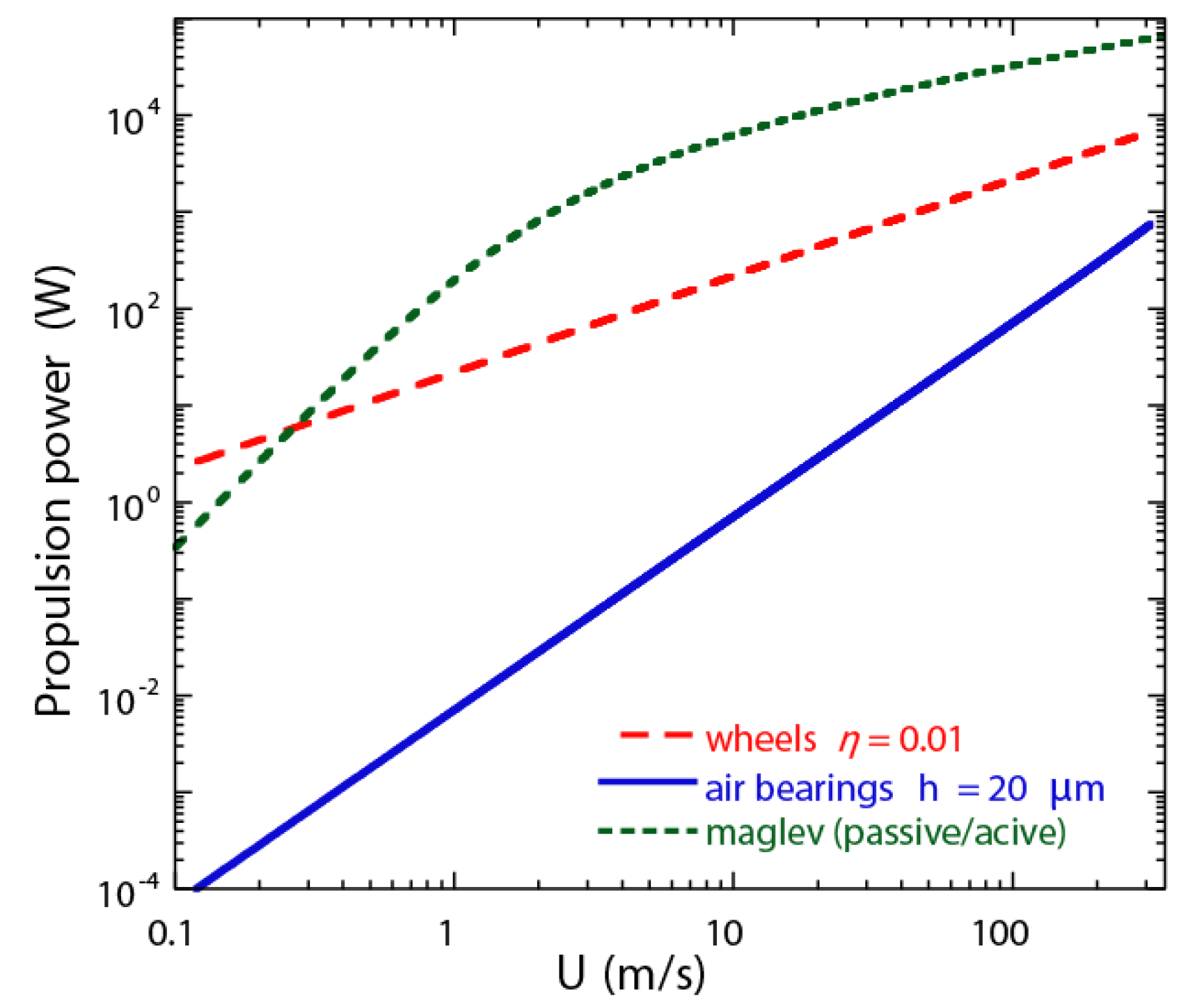
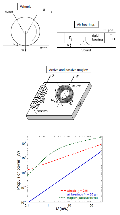
The present work addresses the second drag/friction source in the Hyperloop system, namely the one related to the locomotion and or levitation of the pod in the tube. Currently this can be accomplished in practice by using a method based on one of the following three general classes [
10]: (a) wheel locomotion, (b) air bearing levitation, (c) passive and active magnetic levitation systems; our main objective is to evaluate the level of friction present in each system and hence estimate the required level of power needed to propel a Hyperloop pod at high speeds. Another objective is the extraction of simple scaling laws for power against any parameter of interest, such as vehicle mass, levitation height, mass flowrate required for operation, battery power, etc. Such scaling laws will allow for a quantitative comparison of the three classes of systems, as well as offer design guidelines for practical Hyperloop systems. In what follows we concentrate on the steady-state motion of a Hyperloop system moving at a constant speed
. The dynamic response of each system is, of course, a very interesting topic in itself, but is beyond the scope of this paper; here we are concerned with the calculation of gross propulsive power needed to maintain the Hyperloop system in uniform motion. Propulsion can be affected by applying an external periodic impulse every so often, as proposed originally in Reference [
1], by using linear induction motors, or by carrying an internal propulsion system onboard the Hyperloop pod, e.g., batteries and electric motors.
3. Air Bearings
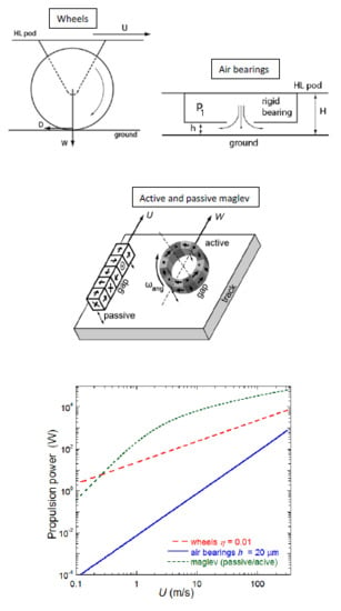
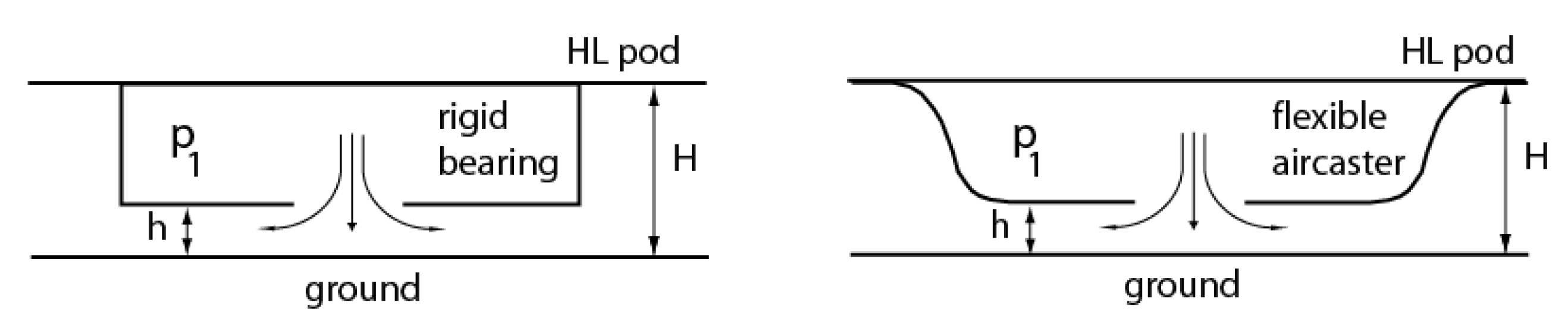
Air bearings are devices that hold gas-usually air-under pressure, and release it through openings or slots in order to create a gap/cushion of air that ‘levitates’ the bearing and whatever weight rests on it. They can be rigid (e.g., ceramic, or metallic) or flexible (e.g., ‘air-casters’), as shown in
Figure 2, and be built in numerous different geometries and configurations, both aerostatic, i.e., levitating and hovering above ground, or aerodynamic, i.e., moving at a constant speed. The drag experienced by an air bearing moving at high velocity can be calculated in a simplified manner following Reference [
12]. The calculation applies to planar, two dimensional (2D) rigid bearings that operate very near the ground, and also to planar air-casters, i.e., flexible bearings, and assumes a lubrication type of air flow in the gap between bearing and ground.
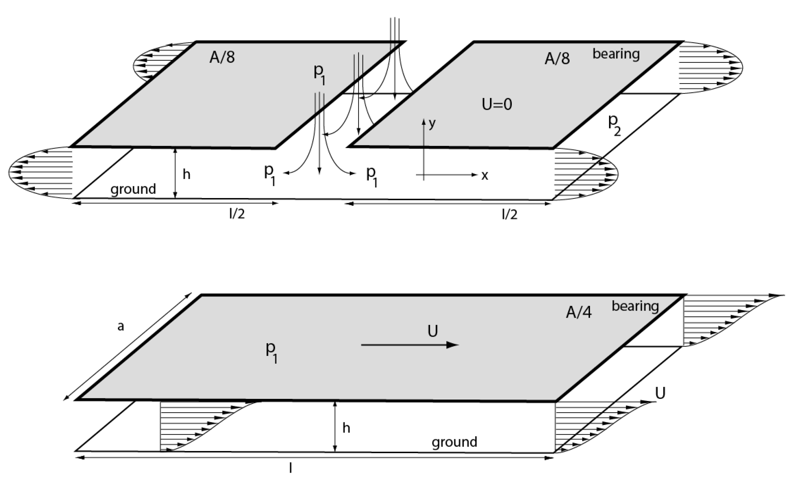
As shown in
Figure 3 the planar configuration is considered here for ease of calculation; realistic devices usually have a cylindrical configuration, with air fed through round openings and moving radially in the gap between bearing and ground. The salient features of the problem are captured well by the planar configuration, and whatever mathematical differences may arise between the two cases are expected to be secondary. The air cushion below the device (gap thickness
) will be small enough to allow for laminar flow at all pod speeds (
), and the Reynolds number of the flow will be small enough for lubrication flow [
13] to be valid in the gap.
The pressure inside the bearing is set to
, while the ambient pressure,
, can be set to atmospheric, or zero in the case of an evacuated Hyperloop tube. Gas (air) is forced under pressure and flows from the bearing inlet to the ambient through the gap, as shown in the top of
Figure 3. A laminar Poiseulle flow will be established on each side of the hovering bearing. The Navier–Stokes equation can be used to calculate the resulting parabolic velocity profile along the perpendicular axis (
y):
where
is the dynamic viscosity of the gas. The mass flowrate of the gas flowing in the gap may be calculated using conservation of mass and assuming constant density
ρ in every location
x:where
is the width of the bearing. The above can be integrated along axis
x to calculate pressure drop across the length of the bearing; furthermore, the ideal gas law is used to relate
,
, and temperature
, to obtain:
where
R is the ideal gas constant and
the length of the bearing. This result, despite inaccuracies due to simplification in geometry and other assumptions inherent in its calculation, showcases one important feature of air bearings: There is strong dependence of all parameters on gap height
h. For any given pressure of operation
the mass flowrate scales as the cubic power of gap thickness
h. This in turn implies that tremendous flowrates are required for levitation at heights of a few millimeters; realistic bearings ‘hover’ at heights of 10–100 μm, and not 5–10 mm as required by practical considerations in the Hyperloop system. In order to increase the levitation height to macroscopic values, and hover for any realistic duration of time the vehicle must store very large quantities of air under extreme pressures.
A numerical example can easily be formed using some realistic values: for
= 5 × 10
5 Pa,
= 10
5 Pa,
T = 300 K,
μ constant for air at 300 K, and
= 20 μm, four square bearings, each with
a=l = 0.1 m require a mass flowrate of almost 10
−5 kg/s. In order for the same four bearings to levitate at a 5mm height (
) a mass flowrate of 150 kg/s would be necessary, a value usually associated with a small rocket engine. Such high values are clearly prohibitive as they would imply storage capabilities similar to those of rockets in order to accomplish Hyperloop levitation of a few minutes. It is also important to note that the overall gap distance between the vehicle and the ground (
, shown in
Figure 2) is not relevant for this calculation. Even for the case of air-casters, the flexible surface must be in very close proximity to the ground (at gap height
) for levitation and locomotion to take place. Therefore, the ground plane must be flat at scales comparable to
, i.e.a few microns, for levitation to take place successfully. This requirement becomes even stricter if we consider that the bearings must maintain such close proximity to the ground while also moving at very high speed.
We may extend the simple calculation to the rest of the scaling parameters of the air bearings necessary for Hyperloop levitation. The load-bearing capability of the levitation system may be estimated from the hovering case (top of
Figure 3). Every one of the four air bearings, each with an area
A/4 can support a weight of
, for a total weight of
=
. The total mass of the vehicle (
m) must be supported by the air bearings (rigid or air-casters) each with a length
l and width
. The average pressure in the area underneath the air bearing can be calculated easily from the above as:
This, in turn, implies that a total weight of 2200 N can be levitated with the four air bearings of the example set up previously.
As shown in the bottom of
Figure 3, when the levitating pod is moving at high speed (
) the flow in the gap resembles that of a planar Couette type [
13]. The top surface corresponds to the bladder surface of the air-casters, or the external surface of a rigid air bearing. We can use a simple calculation to estimate the shear stress at the air bearing surface, and hence the viscous drag generated by the fluid flow. A number of factors may complicate this calculation:
- (a)
Laminar flow in the gap may transition to turbulent flow at high Reynolds numbers. Following the general guidelines set up in Reference [
14] we can see that this is not the case for even the highest speeds expected in a Hyperloop system: the Reynolds number based on the gap height (
) is less than the experimentally determined transition value which lies in the range of 400–1000; The Reynolds number in most cases examined here is smaller than that required for transition to turbulence. Only the highest gap values, at very high speeds (e.g., faster than 150 m/s) correspond to Reynolds numbers larger than 400. Therefore, while we may anticipate the possibility of transition to turbulent flow in the gap leading to higher friction in the case of rough tracks, in reality the concept of levitation using air bearings would become infeasible if the roughness exceeded a few microns; put another way, this levitation method requires very smooth track surfaces that would maintain a laminar flow in the gap at all conditions examined;
- (b)
The flow pattern in the gap is a lot more complicated than the one represented by a simple Couette flow. In reality a combination of the flow patterns shown in the top (velocity
)
and bottom (velocity
) of
Figure 3 is established in the gap at high speeds, since the bearing must be levitated by high pressure air which then combines with the incoming ambient air stream inside the gap. Furthermore, when the Hyperloop track (tube) is under low pressure, the low ambient air density condition may lead to velocity slip at both boundaries, at the bearing wall and on the ground [
15];
- (c)
At high speeds, e.g., Mach numbers higher than 0.3, the flow compressibility effect becomes important. In those conditions the well-known linear Couette flow [
13] is modified slightly to the one shown schematically in the bottom of
Figure 3 [
14]. Changes in the gas velocity profile near the walls result in increase of shear stress and finally a higher drag for the whole system.
We will assume a laminar, incompressible Couette flow inside the gap to evaluate the drag. A laminar friction coefficient
Cf may be evaluated as [
14]:
where
γ is the gas specific heat ratio, and
Ma the Mach number of the gas flow in the gap (
U/α,
α speed of sound.). Finally, the drag (
) due to aerodynamic friction arising from Couette flow may be evaluated as:
where
A is the area where the shear stress is generated, and corresponds to the total area of the air bearings in close proximity to the ground.
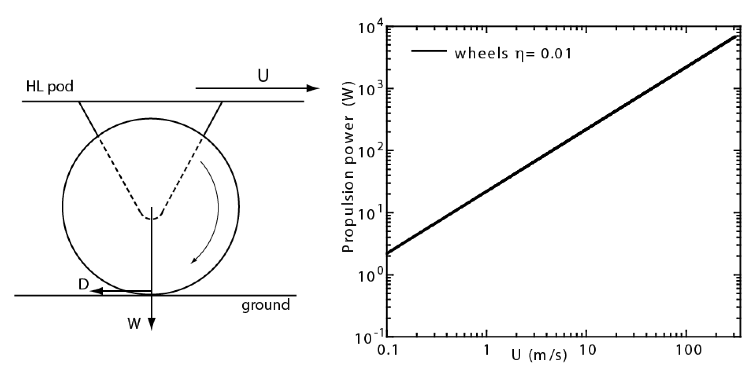
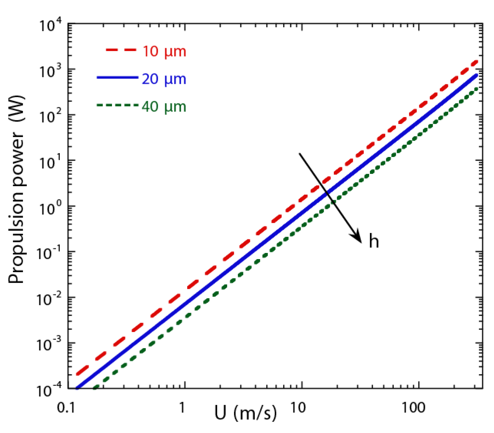
Some means of propulsion must be added to the Hyperloop system, either internal or external to the system, to overcome this drag. The propulsive power can be easily calculated as
as shown in
Figure 4; There, we plot the propulsion power requirement for a vehicle with a total weight of 2200 N at different levitation heights. There is a clear quadratic scaling of power with respect to velocity and an inverse dependence on levitation height (
). As expected, smaller values of
h lead to higher stress at the wall and higher drag/power requirements. At the maximum expected speed of approximately 300 m/s (or Mach 0.9) and a levitation height of 20 μm the required propulsive power is 720 W. Larger values of levitation height would make the required power even smaller, but at the detriment of the required mass flowrate, which would need to be increased drastically.
We can carry out the particular design example of a vehicle with a total mass of 225 kg a little further, by assuming that the pod carries with it a total of 25 kg of air, for a ‘propellant’ mass fraction of 11%, with a tank pressure of 5 bar (
) exhausting to a 1-bar ambient pressure (
). The total hovering time of the vehicle depends on the mass flowrate required for levitation, and this depends strongly on levitation height (
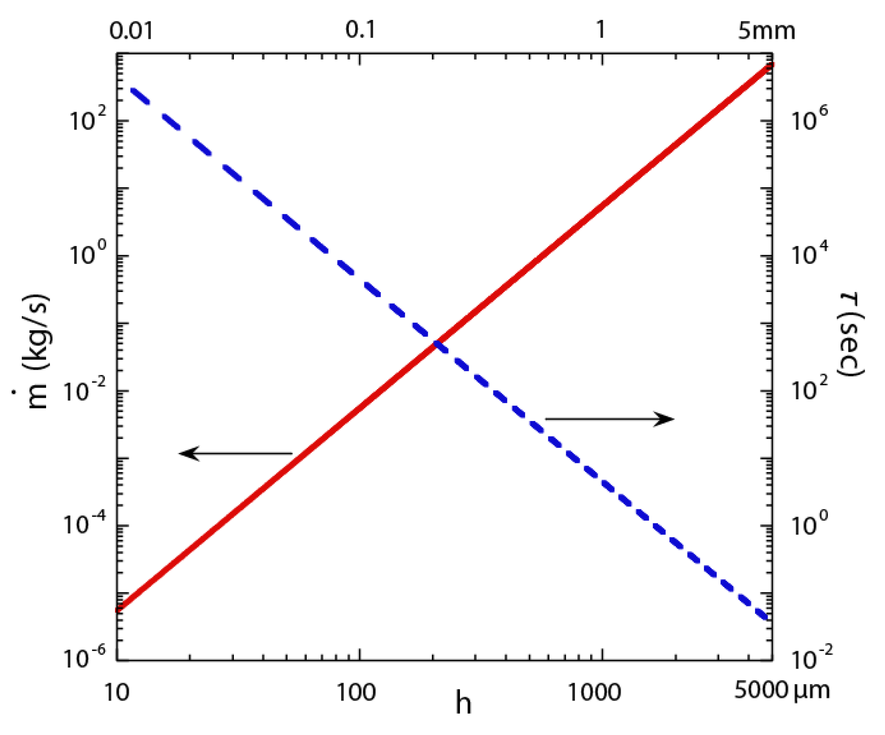
) as shown already.
Figure 5 is presenting both parameters: mass flowrate (
in kg/s) and levitation time
both show a cubic power dependence on gap height
. The results showcase the main issue affecting air bearings, namely the unrealistic mass flowrates that are necessary for levitation at macroscopic heights (in the order of millimeters) and the concomitant drastic reduction of levitation times. Additionally, it is worth noting that the large mass of air necessary for levitation presents further problems with respect to volume: the 25-kg mass must be stored in a 100 L volume under 200-bar pressure; this requires tanks that can withstand the pressure, as well as pressure regulators to reduce the high pressure to the one used in the bearings. Ultimately those additional components must be included in the limited mass budget of the whole system.
One last important design consideration is the scaling of propulsive power with respect to the vehicle weight. The average pressure supporting the air bearings is proportional to the vehicle weight, and approximately proportional to pressure inside the bearings as seen in Equation (4) (
). If everything is kept constant except for the total mass of the vehicle, the Hyperloop pod will need to hover at a lower height that follows the approximate scaling
. Finally, propulsive power in the air bearing scales according to:
4. Passive and Active Electromagnetic Suspension Systems
The final alternative to be covered in this investigation is that of the electromagnetic suspension systems. This technology, although not a completely new and innovative concept, as its application has already been used by various maglev train systems, deserves much attention for its potential capabilities and compatibility with the proposed Hyperloop capsule and tube design.
Much like an aerodynamic suspension design, the concept is based on supporting a vehicle above a track surface, where instead of pressurized air acting as the film lubricant as in the case of an aerodynamic suspension, magnetism from permanent magnets would create this levitation gap. Of course, there would also be existing air between the vehicle and the track, but in this case for simplicity we will assume zero pressure, as would be the case for an evacuated Hyperloop tube. Proposed both in terms of passive and active maglev suspension systems, these technologies could potentially allow the Hyperloop capsule to accomplish its short duration, high-speed travel by eliminating friction due to surface contact. However, as it will be shown subsequently for both systems, another type of friction associated to electromagnetic drag will be produced as a consequence of the generated lift force.
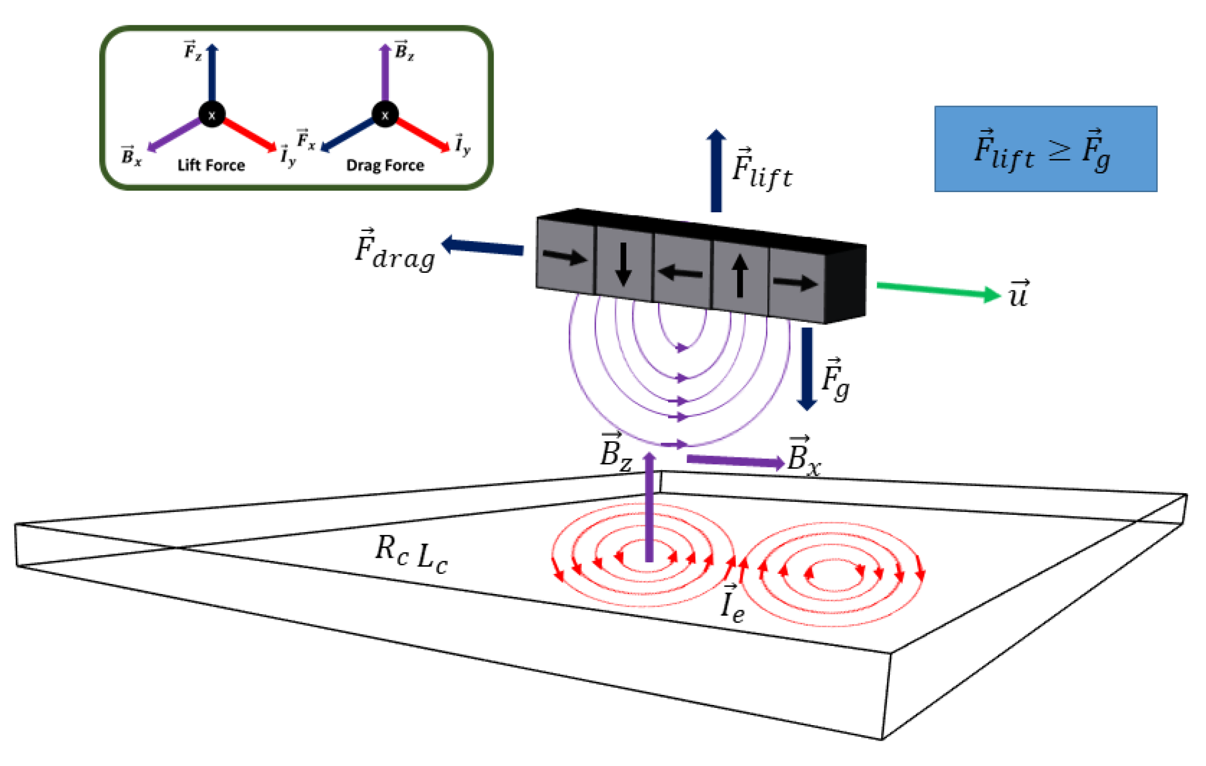
The concept of the electromagnetic passive magnetic levitation system is comprised of various physical phenomena that exploit concepts derived from Maxwell’s equations. The simplest case that can be used to describe the concept of a passive magnetic system is that of a moving permanent magnet along a conducting surface, as represented in
Figure 6.
Table 1 provides a summary of the vector variables shown in
Figure 6. In summary, a permanent magnet traveling with a constant velocity in the
x-direction will emit magnetic field lines along a conducting track surface, which will induce “eddy” currents along the surface (represented in the y-direction), given the track’s self-inductance and resistance properties. The interaction of the magnetic field lines and the induced currents will as a result generate a lift force along the +
z-axis, which will keep the magnets levitated as long as the lift force is equal or greater to the weight of the magnets, or
. Since these models have been explored in the past, e.g., [
16,
17] and references therein, the basic concepts will primarily be summarized in this paper.
Much of the derivation of the electromagnetic passive maglev system follows mathematical models that were developed and investigated originally by the Lawrence Berkeley National Laboratory during the 1980s and 1990s [
16,
17]. By forming a linear Halbach array magnet pattern as shown in
Figure 6, a strong magnetic field can be generated on one side of the magnet and nearly canceled on the opposite side. The two components of the strong magnetic field created by the magnet array can be expressed as [
17]:
where
is the wavenumber of the periodic Halbach array,
the distance traveled by the magnet in the
x-direction,
is the displacement gap between the array and the conducting surface, and
the peak magnetic field of the permanent magnets. The relationship between
and the length of the magnet array,
, is:
Additionally, the peak magnetic field of the permanent magnet arrangement can be calculated as:
where
is the thickness and
the number of permanent magnets in the Halbach array respectively, and
the natural remnant magnetic field of the permanent magnet material [
16].
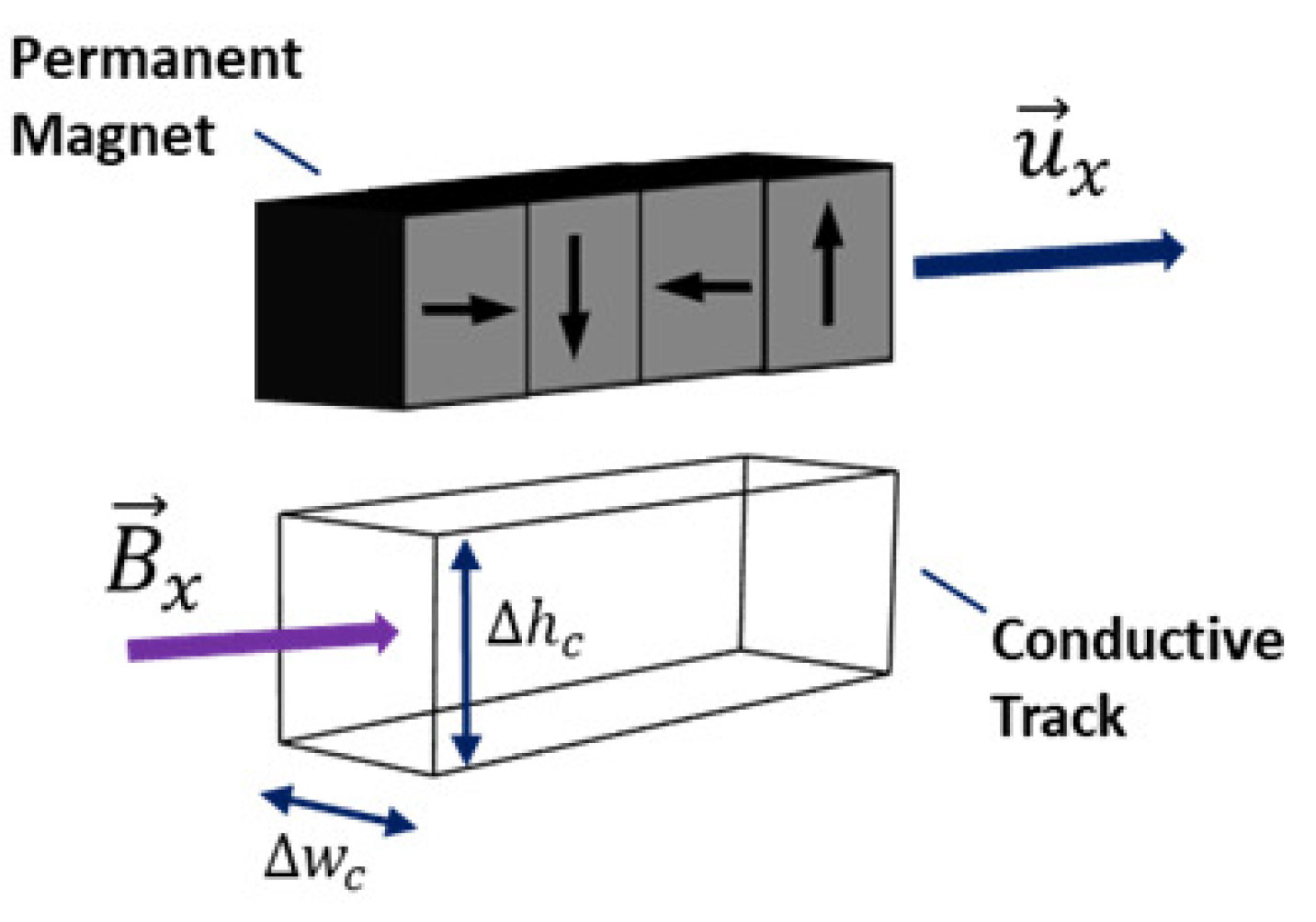
As the permanent magnets travel alongside the conducting track with a given velocity
, this motion will create a change in magnetic flux,
, due to the existing magnetic field vector
in the +
x-direction of the permanent magnet. This is a result of the magnetic field vector traveling through a rectangular cross-section of the conductive track with dimensions
and
, as shown in
Figure 7.
Consequently, the magnetic flux formed by the traveling permanent magnet is directly proportional to the voltage potential that will form within the track surface. This is an effect of Lenz’s Law, which postulates that a change in magnetic flux over time will induce voltage potential,
.
We may rewrite Equation (12) in terms of the electrical current flowing through the conducting surface, along with the resistance (
) and self-inductance (
) of the track, and the excitation frequency of the magnetic flux as a result of the speed of the moving magnetic field vectors,
; the resulting formula can be solved in terms of the existing eddy current within the track,
.
Using the Lorentz force law:
with the magnetic fields in the x and z directions and the eddy current we can evaluate the average lift and drag forces as:
Very often in the literature Equations (15) and (16) are used to represent the overall lift and drag forces, without consideration of the skin depth effect that occurs when excess eddy currents accumulate along the surface and within the track. This idealization is appropriate if one considers a specialized track that has been designed specifically to reduce eddy currents, and where the lift and drag trajectories follow closely the picture described above. However, when comparing these formulas to practical applications using a simple metal conducting slab as a track, such estimations fall short of modeling the proper lift and drag forces with significant offsets in performance output models.
As detailed in Reference [
16] the effect of the skin depth is to reduce the lift force and to increase the drag due to the heating associated with the current inside the material. In all, when taking skin depth
into account for the lift force, we must apply appropriate corrections:
where
represents the maximum lift force when
(or in this case,
, as
.) To derive the skin depth correction in Equation (17) one must make the important assumption that the traveling magnets induce currents primarily to the area projected directly below the magnets, as shown in
Figure 7. Subsequently we will examine this assumption more critically, by comparing this model to published results from a finite-element method (FEM) computation [
18]. A similar correction (not shown here) can be applied to the drag force
in Equation (16)to calculate the effect of skin depth and obtain
. Finally, the ratio of lift over drag
, when considering skin depth is:
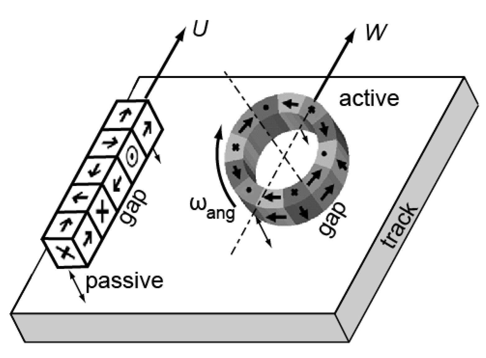
The circular, active maglev system can be considered as derivative of the linear, passive maglev discussed thus far. As can be seen in
Figure 8 the active maglev system functions as a rotational equivalent of the linear Halbach array. Most of the physics is similar between the two systems, and as a result all of the components for formulating lift and drag force as discussed in the previous paragraphs are the same [
19]. The passive maglev consists of a linear Halbach array which moves along the
x-axis with linear velocity
(or
) at a displacement gap (
), and the resultant drag and lift forces depend on
and
as shown already; the active maglev case uses rotary motion and angular velocity
of a circular Halbach magnet array moving in along a circumference to generate lift force. As should become apparent from considering the geometry, the active maglev offers one more degree of freedom, insofar as its linear velocity
W can be controlled independently from its angular velocity
: the latter can be imparted through the use of a high torque motor, while no net motion along the
x-axis is necessary. This is the case of an active maglev system that hovers, stationary, on the conducting track (
while rotating at an angular velocity
; this is related to the velocity
of the linear system and the radius,
, of a circular Halbach array by:
As we have looked at much of the theoretical formulation for the passive-and by extension the active-maglev systems, it is essential to assign actual parameters in order to evaluate the practical performance of the maglev systems and compare to the other levitation/locomotion methods. For the purposes of the present investigation we considered mainly neodymium permanent magnets due to their strong magnetic characteristics; cuboidal magnets of 1-inch side lengths were considered, where a Halbach array pattern could be formed with four magnets per period (
); the material has a natural remnant value of about
1.41. Details of the calculation, which takes into account material properties, can be found in Reference [
20].
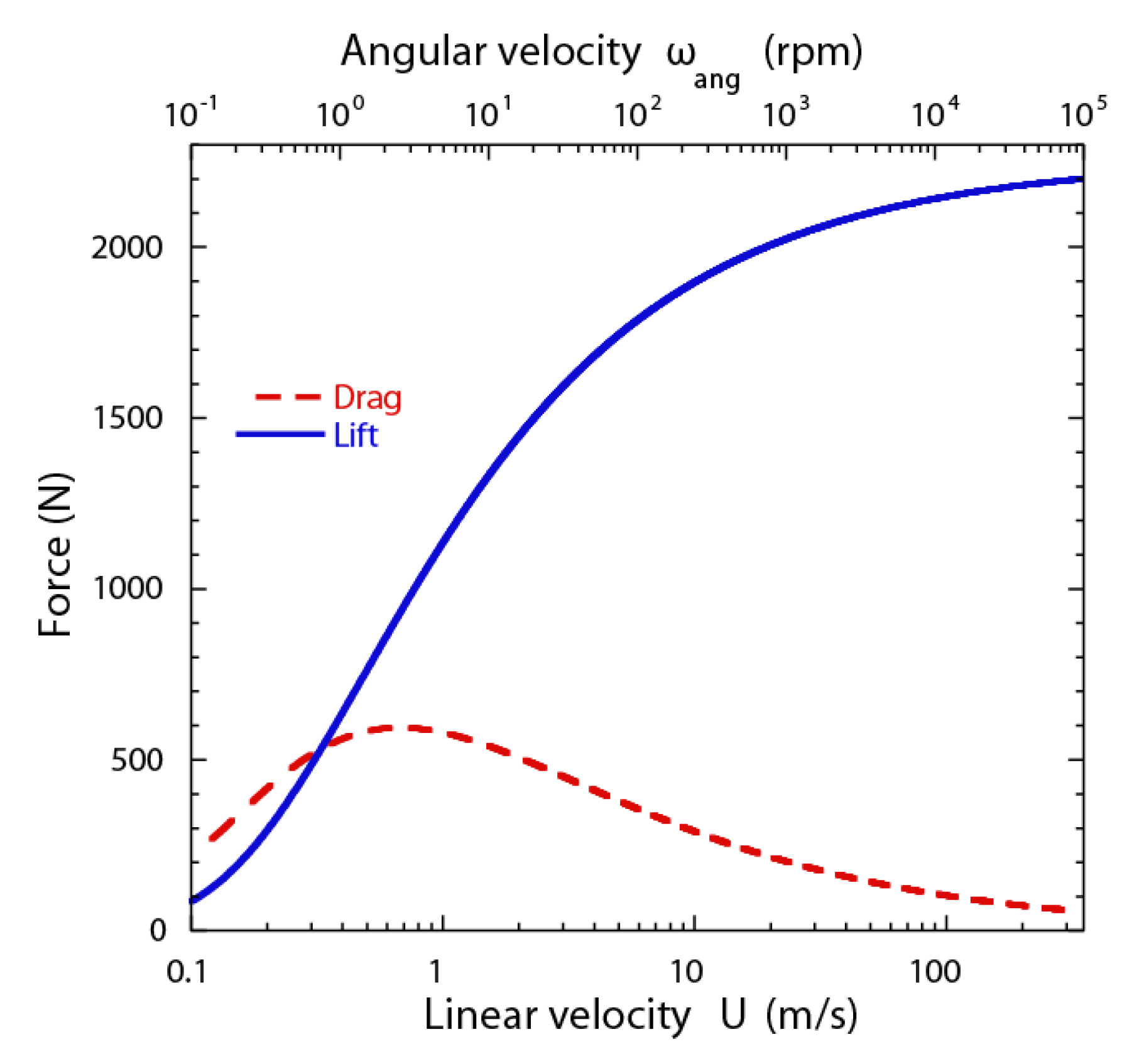
Now, let us consider the case of magnets being used to support a weight of 2200 N, the estimated weight of the proposed Hyperloop pod. If a linear, passive array of magnets were to be placed under the pod at a fixed distance of 10 mm from a simple aluminum conducting track, and sufficient propulsion was provided to the pod, then the lift and drag forces generated by the Halbach array would depend on the pod velocity in the manner shown in
Figure 9. The pod would be able to achieve a velocity of about 340 m/s (760 mph, or Mach 1) but the weight that could be supported changes throughout the trajectory, very rapidly at small speeds (<10 m/s) and more modestly at higher speeds (>50 m/s).
Figure 9 also plots the equivalent result for an active hovering (
) maglev; assuming a motor with a rotational Halbach array of radius 89 mm, the lift and drag forces versus radial velocity
can be calculated using Equations (17)–(20). As can be seen from the plot, the Halbach array parameters chosen could result in the generation of a 2200-N lift at a rotational speed of 10
5 rpm, at a hovering height (gap) of approximately 10 mm. At a fixed hovering height, increase in the angular speed results in monotonic increase of the lift force, but non-monotonic decrease of the drag force.
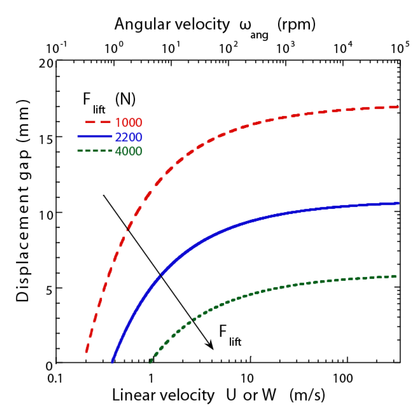
To make a workable passive maglev system the magnets must be capable of lifting the full weight of the pod (2200 N) throughout the trajectory. In order to achieve such a supporting force, a key factor for the system to work is the ability to keep the magnets at a varying, close distance to the track. In other words, there is a relationship connecting the displacement gap between magnets and track, and the amount of lift force that the magnets will be able to support. Such a relationship is shown in
Figure 10, where it is shown that, at a fixed speed, the smaller the displacement gap the stronger the lift force will be, and conversely, the larger the gap, the weaker the lift force. This implies that a pod weighing 2200 N will levitate at very small distances from the track initially, and the gap distance will increase as the pod speed increases. In all, a displacement gap of approximately 10 mm is achievable only at speeds higher than 50 m/s (or approximately 112 mph). In practice a working Hyperloop pod using a passive maglev system like the one described here would require an auxiliary system of wheels that can support the full weight in the initial phase of the trajectory, before the pod speed has increased sufficiently for the passive maglev to support the weight.
As before,
Figure 10 presents the equivalent calculation for a hovering active rotary maglev system: the varying displacement gap is, in this case, the hovering height of the system, and it is presented as a function of angular speed for three different Hyperloop pod weights. As intuitively expected, the heavier pods will hover closer to the track if the fixed angular speed stays fixed; conversely, increasing the angular speed increases the displacement gap for any given lift force (or pod weight).
As shown in
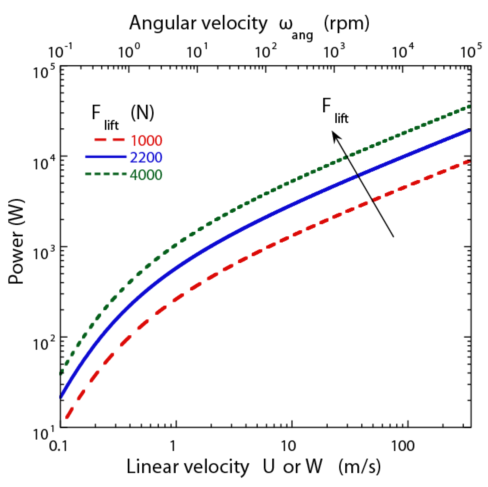
Figure 9 drag force is always generated by a maglev system at the same time as it generates lift force. The power associated with the drag force must be provided by an external propulsion source, and is therefore a very important metric of performance/cost factor for the passive maglev levitation system. Absent air drag inside the tube, this propulsive power loss can be derived by multiplying the drag force times the linear velocity of the system:
Figure 11 provides the relationship between propulsion power and the linear speed of the system. In terms of lift force capability, the power required to propel the passive maglev system is proportional to the mass (weight) of the Hyperloop pod.
We may extend this model further to determine the battery power consumption of an active maglev system, as is also shown in
Figure 11. In the case of the active rotary maglev system Equation (14) still applies, and provides the required power as the product of torque and rotational velocity
. This term may be interpreted as the onboard battery power required by the motor used in rotating the circular Halbach magnet array.
Figure 11 presents the results on battery power consumption for three possible pod weights, plotted against angular speed
(top abscissa). According to this model, everything else being equal (rpm, magnets, etc.) the lighter pods require less battery power and levitate at larger heights.
This result describes the specific case of an active maglev levitation system hovering at a given height above the track due to its rotational velocity (
) and incurring a ‘penalty’ in battery power (
). At the same time, the active maglev may move along the track at an axial velocity (
) similar to its passive counterpart. Such a motion would also generate electromagnetic drag, and consequently power loss that must be supplied by external propulsion. Finally, we may estimate the power requirement for an active maglev by simply equating the two axial velocities (
) and assuming that Equation (20) holds for the active maglev as well. The result is shown in
Figure 11, where the bottom abscissa is now axial velocity
, and the vertical axis propulsive power required by the active maglev. It should be noted that an accurate calculation of propulsive power loss for the active maglev is more complicated, since one must also account for the interaction between the electromagnetic drag forces along the axis as well as along the circumference of the array of magnets. For the purposes of the present study the propulsive power just presented serves as an adequate estimate. In both cases of passive as well as active maglev systems we can see a clear difference in behavior between the low-speed and high-speed regions; this result, which is evident in
Figure 11, is due to the relative reduction of electromagnetic drag at high speeds, as seen in
Figure 9. At near-sonic speeds, the required propulsive power scales almost as a square root of the velocity (
,
).
The simple model of the linear, passive maglev described here depends on some crucial assumptions, most importantly on the existence of a constant skin depth
. In order to gain some confidence in the behavior of the model we conducted a comparison between its results and those of a FEM electromagnetic simulation published in Reference [
18]. There, the authors present a careful study of the electrodynamic suspension system that may be used in the Hyperloop pod, and examine the particular case of a vehicle designed and built at the Swiss Federal Institute of Technology (ETH) Zurich. They first present a simple model, similar to the one in this work, which examines the theoretical scaling of lift and drag force over an infinite domain, and then provide 2D and 3D FEM electromagnetic simulations of the interacting field between a linear Halbach array and a simple slab track. We compared the results of our model to the most accurate simulation (3D FEM) results in Reference [
18] by using the physical parameters (e.g., magnets, sizes, levitation height, etc.) of the computation.
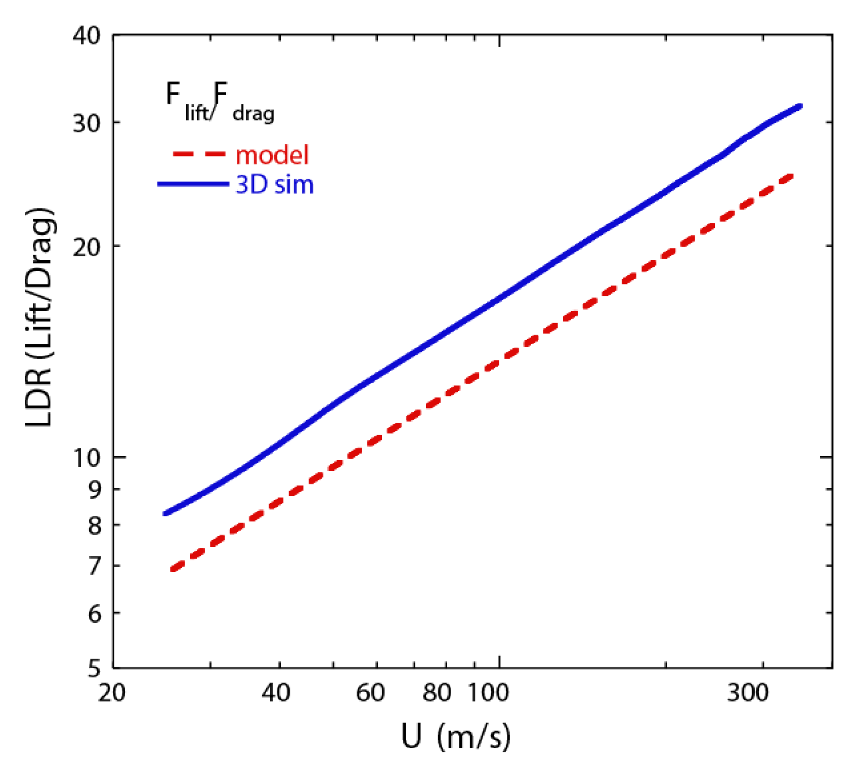
Specifically, we examined the Lift/Drag force ratio (
) from Equation (19) as a function of axial velocity
. The results, presented in
Figure 12, show that both the model developed here, as well as the 3D simulation results in Reference [
18] capture exactly the expected theoretical trend of a power law with an exponent of 0.5. At the same time, our model shows a consistent bias of approximately 25% within the whole range of axial velocities, for the case Lift/Drag ratio. This discrepancy is likely due to the simplicity of our model, which assumes that effects of the magnetic field vector into the conducting track are confined inside a simple cuboidal region (
Figure 7). Still, the agreement is quite sufficient for model validation, and allows us to use the simple algebraic model developed here, instead of more elaborate simulations, in design calculations.
Finally, in order to gain further confidence in the electromagnetic model presented in this work we conducted a comparison between model predictions of levitation time and battery power requirements against the only-to our knowledge-published results from an active maglev levitation system; these can be found in the patent disclosure of Arx Pax LLC, San Jose, CA, a company that designed and built a prototype rotary levitation system for the Hendo hoverboard [
21]. The comparison (not shown here) showed adequate agreement, with discrepancies in the range of 2–15%, which led to the conclusion that our model also captures adequately the behavior of the rotary, active maglev system.


