Abstract
Gas hydrates have great potential as future energy resources. Several productivity and stability analyses have been conducted for the Ulleung Basin, and the depressurization method is being considered for production. Under depressurization, ground settlement occurs near the wellbore and axial stress develops. For a safe production test, it is essential to perform a stability analysis for the wellbore and hydrate-bearing sediments. In this study, the development of axial stress on the wellbore was investigated considering the coupling stiffness of the interface between the wellbore and sediment. A coupling stiffness model, which can consider both confining stress and slippage phenomena, was suggested and applied in a numerical simulation. Parametric analyses were conducted to investigate the effects of coupling stiffness and slippage on axial stress development. The results show that shear coupling stiffness has a significant effect on wellbore stability, while normal coupling stiffness has a minor effect. In addition, the maximum axial stress of the well bore has an upper limit depending on the magnitude of the confining stress, and the axial stress converges to this upper limit due to slipping at the interface. The results can be used as fundamental data for the design of wellbore under depressurization-based gas production.
1. Introduction
Gas hydrates are solid crystalline compounds which consist of water and guest molecules [1]. Gas hydrates are formed under certain sets of high pressure and low temperature conditions, outside of which the gas and water species typically remain in separate phases [2]. The guest molecules are gas molecules such as methane, ethane, propane, or carbon dioxide. These guest molecules are combined by hydrogen-bonded water. This natural gas is a premium fuel because it burns cleanly and produces less carbon dioxide [3]. According to the latest research, approximately 230 natural gas hydrate deposits have been investigated globally, with reserves of about 1.5 × 10¹⁵ m3 of natural gas [4]. Most natural gas hydrate deposits appears to be in the form of ‘structure I’, with methane as the trapped guest molecule, and its fraction is more than 90% [5,6].
Methane hydrate is also an important future energy resource for South Korea. The national projects, Ulleung Basin gas hydrate expeditions 1 and 2 (UBGH1 in 2007 and UBGH2 in 2010), were conducted to investigate the hydrate reserves and characteristics of gas hydrate-bearing sediments of the Ulleung Basin in the East sea of Korea [7,8,9]. Based on the data of UBGH2, the estimated amount of natural gas-hydrate deposits in Ulleung Basin ranged from 4.4 × 10⁶ to 9.2 × 10⁹ m3 [10,11,12]. Recently, Bo et al. [13] suggested deterministic estimation from rock physics modeling and pre-stack inversion, and estimated the total gas-hydrate and gas resource volume in Ulleung Basin as about 8.43 × 10⁸ m3 and 1.38 × 10¹¹ m3, respectively. These amounts can provide usable energy for more than thirty years to the whole nation.
Several methods of dissociating the gas hydrate from the hydrate-bearing sediment (HBS) have been suggested; thermal or inhibitor injection, depressurization, CO2/CH4 exchange and combinations of these are representative production methods [14,15]. The main mechanisms of production methods are to dissociate the hydrate in the form of ice-crystals to a gaseous or liquid state by increasing the temperature or lowering the pressure. Among other methods, depressurization is the most common method, and has been applied as a major method of production for the field test (e.g., Mallik site in 2002, Nankai Trough in 2013) for gas hydrate production in the reservoir [16,17].
During depressurization to dissociate the methane gas from HBSs, significant ground settlement occurs. This is because of the strength and stiffness reduction induced by the phase change of hydrate (e.g., the state of hydrate converts from ice crystal state to liquid or gaseous state), and the increase of effective stress, which is the stress carried by the soil. Field test for gas hydrate production has several technical problem according to the complexity of mechanism aforementioned, and needs huge budget. Thus, it is essential to perform the numerical analysis to ensure the productivity of gas hydrate and stability of production facilities before the field test. Thermal-hydraulic-mechanical (THM) coupled numerical analysis should be performed to simulate the mechanism of gas hydrate production [18]. Several numerical coupled simulators based on kinetic and equilibrium model have been developed (e.g., TOUGH+Hydrate [19], HydrateResSim [20], MH21 [21], and STOMP-HYD-KE [22]). Kim et al. [23,24] also developed the THM coupled simulator using FLAC3D, and verified with cylindrical core experimental data [25]. The input parameters (e.g., boundary condition, intrinsic hydrate reaction rate, intrinsic permeability, initial hydrate saturation, overall heat conductivity, wellbore heating temperature, bottom hole pressure, etc.) and constitutive models (e.g., permeability model, stiffness model, and heat transfer model) for numerical analysis significantly affects both the energy recovery potential and geological hazards prevention [26,27,28]. Kim et al. [26] provided a comprehensive estimation for model parameters and properties based on vast data from field seismic surveys in Ulleung basin and laboratory experimental results. Numerical studies on the efficiency and productivity of gas hydrate production have been carried out continuously, while stability analysis for the hydrate-bearing sediments or wellbore has not been much considered, although stability analysis is essential to field production [29,30,31,32,33,34].
As depressurization is applied in a sediment, frictional forces are evolved at the interface between the production wellbore and the soil layer due to the stiffness differences of materials. These frictional forces result in axial stresses induced on the production wellbore [35,36,37]. For this reason, soil–structure interaction (SSI) analysis should be conducted before the field test to properly evaluate the stability of the wellbore and HBS. The concepts of shear and normal coupling stiffness (also called interface stiffness) based on the linear Coulomb shear strength criterion are widely used to simulate interfacial stress behavior in numerical analysis [38]. The non-linear behavior of the soil–structure interface and the displacement behavior were investigated according to the interface models [39]. However, there is not much research on the stability analysis of the interface between the production wellbore and HBSs, which is related to the complex mechanism of gas hydrate production in the oceanic environment. Only a few studies have considered the wellbore stability during gas hydrate production [24]. Geological stability was assessed for vertical and horizontal well production scenarios from a displacement perspective [40]. Numerical analyses were performed to investigate the geomechanical behavior of HBS (e.g., pressure, temperature, hydrate saturation, and volumetric stain) and wellbore stability during methane production [24,41]. Kim et al. [24] also restrictively considered the interface properties related to the interaction behavior between the sediment and wellbore. Previous studies have conducted the numerical analysis using the interface model, which considers mainly stiffness of sediments ignoring the confining stress change. The stability analysis during gas hydrate production has to consider the variation of confining stress according to depressurization. However, the research which conducted the stability analysis considering confining stress on interface model has not been published yet.
In this study, the authors investigated the effects of coupling stiffness and slippage phenomena on the stability of the wellbore under gas hydrate production. The present paper describes the concept of coupling stiffness, and the limitation of coupling stiffness model used in FLAC3D. The coupling stiffness models considering the confining stress were derived from the results of experimental tests using artificial Ulleung basin specimen, and applied to the T-H-M simulator developed in previous research [24]. Qualitative numerical analyses were performed to investigate the effects of coupling stiffness and slippage phenomena on the stability of wellbore under depressurization. More specifically, parametric analysis was conducted to investigate the trend of the development of axial stress according to the shear and normal coupling stiffness, and effects of slippage phenomena on the evolution of axial stress of wellbore. Additionally, the relationship between the development of axial stress on wellbore and geotechnical behavior of hydrate bearing sediments under depressurization was investigated.
2. Thermal–Hydraulic–Mechanical Simulation for Wellbore Stability
The mechanism of gas hydrate production from hydrate bearing sediments (HBS) is the complex reaction related to thermal, hydraulic, and mechanical (T-H-M) behaviors. This section will provide a brief description of the constitutive models for the T-H-M simulator, which was developed by Kim et al. [24]. An explanation is also provided of the limitations of the existing coupling stiffness model used in the FLAC3D software, with a suggestion for a new linear regression model derived through experimental tests. Additionally, the concept of stress evolution to consider the slippage at the interface is described.
2.1. Thermal–Hydraulic–Mechanical Coupled Simulator
Constitutive Models for T-H-M Simulator
In this study, a three-dimensional T-H-M coupled simulator, which was developed by Kim et al. [24], was used for evaluating the development of axial stress on the wellbore. The T-H-M simulator is based on the commercial finite difference method program, FLAC3D. By solving coupled thermal, hydraulic, and mechanical constitutive models, the T-H-M coupled simulator can model phase behavior, flow of fluids and heat transfer of hydrate deposit. The constitutive models used for simulated T-H-M are briefly described in this section. An elastoplastic Mohr-Columb model is used in the mechanical analysis. To consider the phase behavior, equilibrium hydrate pressure (Pe) and the corresponding temperature (T) are calculated by Kamath’s equation [42]:
where Pe is the equilibrium hydrate pressure (kPa), Τ is the temperature corresponding to pressure (K), and the model parameters α and β are 42.047 and −9332, respectively. The rate of hydrate decomposition can be estimated [43]:
where ng is the moles of methane in the hydrate, Kd is the kinetic constant (mol m−2Pa−1s−1), As is the specific surface area of the hydrate-bearing sediment (3.75 × 10⁵ m2), n is the porosity, Sh is the hydrate saturation, Pe is the equilibrium pressure (kPa), P is the present pressure (kPa), K0 is the intrinsic kinetic constant (1.24 × 10⁵ mol m−2Pa−1s−1), ΔEa is the activation energy, R is the gas constant (8.314 J mol−1K−1), and T is the temperature (K). A specific value, , was applied in this study.
Multi-phase flow was modeled by Darcy’s law [44] and the relative permeability of gas and water were considered by van Genuchten model (1980) [45]:
where is the relative permeability of water, is the relative permeability of methane gas, and Se is the effective saturation. And a, b, and c are the van Genuchten parameters. The dissociating process of hydrate is endothermic reaction. To consider the thermal reaction, the energy balance equation was used as follows:
where ΔT is the change in temperature per unit time (K), cT is the effective specific heat (J/kg/K), q is the seepage-velocity vector (m/s), ρ is the density (kg/m3), and c is the specific heat (J/kg/K), and the hydrate dissociation enthalpy change ΔH is 56.9 kJ/mol. The subscripts s, g, w, and h represent the soil, gas, water, and hydrate, respectively. More detailed overall of development and verification of T-H-M simulator had been described in Kim et al. [23,24].
2.2. Interface Model
2.2.1. Concept of Force Transfer at the Interface
During dissociation of methane hydrate from HBS by the depressurization method, ground settlement can occur due to the increase of effective stress, which is induced by decreasing the pore water pressure. At this moment, the frictional forces are generated at the interface between the production wellbore and the soil layer due to the stiffness difference of material, and draws the production wellbore. Therefore, it is essential to consider the interface characteristics for accurate stability analysis of wellbore during depressurization method. The concepts of shear and normal coupling stiffness (also called interface stiffness) have been widely used in numerical analysis to consider the interface characteristics [39,46,47]. In this study, the FLAC3D was used to estimate the wellbore stability considering the interface characteristics under the methane hydrate production. FLAC3D provides interfaces that are characterized by Coulomb sliding and/or tensile and shear bonding. The normal and shear forces at the interface are determined at calculation time () through the following equations:
where , and are the normal and shear forces (N) at time (), respectively. is the absolute normal penetration of the interface node into the target face (m), and is the incremental relative shear displacement vector (m). is the additional normal stress added due to interface stress (Pa), and is the additional shear stress vector due to interface stress initialization. and are the normal and shear stiffness (Pa/m). A is the representative area associated with the interface node (m2) [38]. The normal and shear coupling stiffness act like spring constants at the interface. The concept of load transfer at the interface considering the coupling stiffness in numerical analysis is as shown in Figure 1.
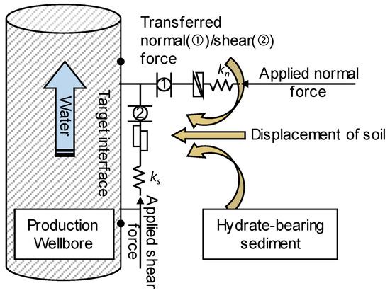
Figure 1.
Concept of transferring the normal and shear stress at the interface under the depressurization method.
2.2.2. Coupling Stiffness Model in FLAC3D
The shear and normal coupling stiffness are usually determined experimentally by measuring the stress and deformation through the direct shear test or triaxial test [46,48]. In FLAC3D, the shear and normal coupling stiffness to estimate the frictional force are derived by empirical model (Equation (11)). This model is a function of the bulk and shear modulus of soil, and considers that the shear and normal coupling stiffness has equal value:
where ks, kn are shear coupling stiffness and normal coupling stiffness (MPa/m), respectively; K and G are bulk and shear modulus (MPa), respectively; zmin is the smallest width of an adjoining zone in the normal direction; and the max [ ] notation indicates that the maximum value over all zones adjacent to the interface is to be used [38]. While the coupling stiffness model used in FLAC3D considers only the stiffness of soil, it reveals that the normal and shear coupling stiffness are largely affected by the interface properties (i.e., confining stress, roughness, interfacial cohesion, interfacial friction angle, etc.) [49]. In particular, many studies have found that confining stress has a significant effect on the coupling stiffness through experimental tests [48,49]. Therefore, it is necessary for the interface model to consider confining stress for accurate stability analysis of the wellbore.
2.2.3. Linear Regression Models from Lab-Scale Experimental Tests
Laboratory-scale tests were performed to investigate the correlation between shear and normal coupling stiffness with confining stress. Direct shear tests, which consider the shearing interface between the wellbore and sediment, were conducted to evaluate the shear coupling stiffness. Figure 2a shows experiment set-up of direct shear test. In this experiments, artificial specimen of the Ulleung Basin core sample, which has D10 = 52 um, D30 = 90 um, D60 = 145 um, was used to simulatethe sediments of the pilot test site (UBGH2-6) and a STS316L disk was used as production wellbore surface. During the shearing, confining stress was maintained with measuring displacement and load. In addition, consolidation tests were conducted to determine the effect of confining stress on the normal coupling stiffness. Displacement was measured while axial stress was applied on the top of specimen. Figure 2b presents simple diagram of experiment set-up of consolidation tests on the simulated interface between artificial specimen and wellbore surface. Normal stress was applied until 650 kPa with measuring displacement of the specimen. The experiment was repeated with various specimen height from 30 mm to 70 mm.
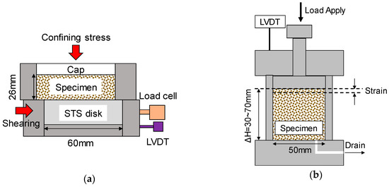
Figure 2.
Schematic diagram of lab-scale tests: (a) direct shear test; (b) consolidation test.
Figure 3a shows measured data of shear stress and displacement while shearing wellbore surface and sediments. The shear coupling stiffness can be derived from the measured data from the slope of the relationship between shear stress and displacement. The slope was calculated from the peak shear stress point which represents highest stiffness level at the residual stress condition. Figure 3a shows that the shear coupling stiffness increases with the increment of confining stress.
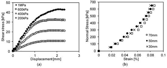
Figure 3.
Results of lab-scale tests: (a) stress-displacement curve of the consolidation test; (b) stress-strain curve of the direct shear test.
Figure 3b shows the expressed stress with the strain rate instead of displacement because displacement is affected by size of the specimen. Interface stiffness is calculated as stress divided by displacement, which is derived from strain. The effective distance concept was utilized to convert strain into displacement, where the diameter of the production wellbore was considered as the effective distance.
The linear regression interface models derived from the experimental data are as shown in Figure 4. The shear and normal coupling stiffness have a linear trend with the confining stress. The models of the shear and normal coupling stiffness considering confining stress are as shown in Equations (12) and (13):
where σ’c is confining stress (MPa).
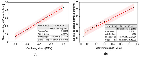
Figure 4.
Linear regression models with confining stress: (a) shear coupling stiffness model; (b) normal coupling stiffness model.
The proposed models and existing model used in FLAC3D were compared. As shown in Figure 5, the existing model shows a constant value with confining stress because it is a function only for the modulus. In contrast, the proposed models show linear trends with confining stress, and estimate the shear and normal coupling stiffness differently. Through the results of the direct shear test and consolidation test, it is regarded that it is more reasonable to use the proposed models for simulating the stability analysis of interface behavior.
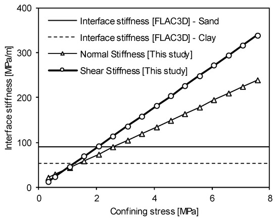
Figure 5.
Comparison of interface stiffness models.
2.3. Slippage at the Interface
2.3.1. Concept of Wellbore Stress Evolution
During production of methane gas from the HBS under the depressurization method, hydrate-bearing sediment is settled with the increase of effective stress. According to Equation 10, the transferred shear stress at the interface is a function of coupling stiffness, shear deformation, shear stress vector, and skin area. Therefore, the transferred shear stress at the interface is proportional to the ground subsidence due to the shear deformation term. This leads to development of the axial stress on the wellbore due to the normal and shear coupling stiffness during ground subsidence. According to the Coulomb stress-strength criterion, the shear stress at the interface cannot exceed the shear strength of soil (Figure 6). Therefore, the shear failure at the interface occurs when the shear stress at the interface reaches the shear strength. After the shear failure of the sediments, the friction between the sediments and wellbore is constant, and there is no additional evolution of axial stress on the wellbore due to the slippage phenomenon on the interface.
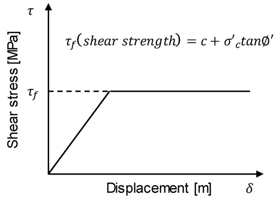
Figure 6.
Comparison of interface stiffness models.
2.3.2. Maximum Axial Stress
The axial stress on the production wellbore, which is induced by the compaction of sediments, cannot be developed over the specific upper bound value according to the Coulomb stress-strength criterion. This critical stress value is defined as the maximum axial stress in this study. The maximum axial stress on the wellbore varies with confining stress during depressurization because the axial stress on the wellbore is a function of the confining stress. The axial stress is developed by the shear stress on the interface area induced by ground subsidence. The maximum axial stress is derived in the following order. At first, axial stress on the wellbore, (Pa), can be estimated as follows:
where () is the shear stress (Pa), usi is the displacement in shear direction (m), is the skin area (m2), and is the cross-section area of wellbore (m2). When the shear stress reaches the shear strength of sediments, slippage occurs and the axial stress at this time is the maximum axial stress. Therefore, the maximum axial stress can be expressed as:
where is the maximum axial stress of the wellbore (Pa), and () is the shear strength in each production period (Pa), c is the cohesion (Pa), is the confining stress (Pa), and is the friction angle (). Because the shear stress cannot exceed the shear strength of sediments, the maximum axial stress converges to a specific value of constant confining stress. However, even in the same sediment, the shear strength depends on the confining stress, because the shear strength is a function of confining stress. This means that the maximum axial stress can vary with the confining stress.
2.4. Algorithm for Stability Analysis of the Wellbore
Procedure for Estimating the Axial Stress on the Wellbore
The present paper suggests an algorithm for estimating the axial stress on the wellbore. The proposed algorithm consists of the aforementioned constitutive models and the algorithm for simulating the mechanism of the depressurization method. The flow chart of the proposed algorithm is shown in Figure 7. The detailed descriptions of each stage are as follows. At the first stage, initial shear and normal coupling stiffness are evaluated through the initial confining stress near the wellbore. Second, shear and normal coupling stiffness are updated with changes of pore pressure and effective stress by depressurization. Third, shear strengths of sediments are evaluated according to the updated parameters and maximum axial stresses are calculated by shear strength. Fourth, the maximum stress and axial stress, which is induced by the settlements of HBS, are compared. If the axial stress generated by the subsidence is larger than the maximum axial stress, then shear coupling stiffness is set to zero in order to simulate the slippage between the wellbore and sediments. Otherwise shear coupling stress remains at the same value as in the previous stage and the procedure of depressurization is continued. These procedures iterate until the analytical flow time is equal to the target time.
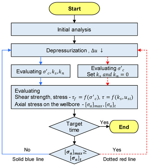
Figure 7.
Algorithm for well-bore stability analysis of simulator.
2.5. Target Site and Input Parameters
Geotechnical engineers in Korea have searched for potential testbed sites for producing gas hydrate and researched mechanisms during production. UBGH2-6 is one of the sites explored during the UBGH2 project and has been established as a pilot test site. The geometry of UBGH2-6 and structure of the production well are shown in Figure 8. The HBS is located at 140 to 160 mbsf (meters below sea floor) and methane hydrate is buried in sand layers in this range. The depressurization method was selected as the production method. From the previous research, it is revealed that the productivity of gas hydrate and stability of hydrate-bearing sediments are significantly affected by bottom hole pressure (BHP), and the appropriate bottom hole pressure for the pilot test is 9 MPa for Ulleung basin [24]. For this reason, we decided UBGH2-6 as a target site for stability analysis, and depressurization method as a production method. The depressurization was conducted in the depth range from 140 to 160 mbsf with a depressurization rate of 0.5 MPa/h until the bottom hole pressure (BHP) was 9 MPa. The input parameters (i.e., properties of wellbore, mechanical, hydraulic, and thermal properties of HBS) for the numerical analysis were taken from Kim et al. [24,26], and are summarized in Table 1 and Table 2.
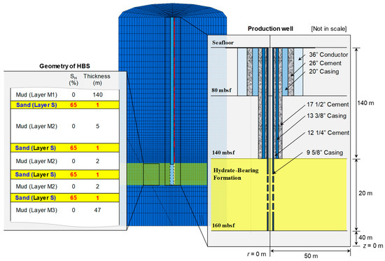
Figure 8.
Schematic diagram of modeled geometry, hydrate-bearing sediment (HBS), and casing structure [24].

Table 1.
Mechanical properties of the wellbore [24].
Table 2.
Thermal, hydraulic, and mechanical input properties used in this study [26].
3. Results and Analysis
This section describes the results of stability analysis of HBS and the parametric study to evaluate the effectiveness of each parameter. The first part of this section shows the results of the stability analysis of HBS during gas hydrate production and describes the relationship between the geotechnical behavior and axial stress evolution on the wellbore. The second section shows the results of the parametric study regarding the effects of coupling stiffness and confining stress on the axial stress of the wellbore. The third section shows the effects of the slippage at the interface on the axial stress.
3.1. Stability Analysis of HBS During Gas Hydrate Production
Geotechnical Behaviors Near the Wellbore During Gas Production
This section describes the effects of geotechnical behavior on the development of axial stress on the wellbore. The ground subsidence occurs due to increased effective stress during the gas hydrate production from the hydrate bearing sediments (HBS). The stability analysis of HBS was performed to examine the geotechnical behavior during gas hydrate production, and to determine the relationship between the geotechnical behavior and evolution of axial stress on the wellbore. The coupling stiffness model of FLAC3D (Equation (11)) was applied in this stability analysis. As shown in Figure 9, x-axis displacements (i.e., lateral displacement) increase during depressurization. Until 12 hours after depressurization, no significant lateral displacements were observed. At 30 days after the beginning of gas production, the maximum lateral displacements of about 0.04 m occurred on both sides of wellbore at HBS.
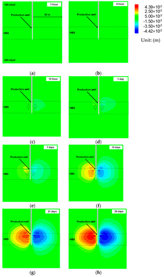
Figure 9.
Distribution of x-axis displacement with production period: (a) after 1 hour; (b) after 6 hours; (c) after 12 hours; (d) after 1 day; (e) after 7 days; (f) after 14 days; (g) after 21 days; (h) after 30 days.
Additionally, ground subsidence and heave occur with dissociation of hydrate as shown in Figure 10. Ground subsidence occurs from the seafloor at initial stage of depressurization. From 7 days after depressurization, ground heave occurs because of suction pressure (i.e., depressurization rate, 0.5 MPa/h) near the production well. The maximum value of subsidence occurs about 0.22 m at the seafloor, and the maximum value of heave occurs about 0.03 m at the bottom of the production well. The aforementioned maximum displacement of HBS is about 0.22 m and is 1.1% of the total depth of HBS. Despite the relatively small displacement, the large axial stress on the production wellbore can occur due to the high elastic modulus of the wellbore. From the distribution of x- and z-axis displacements, it can be deduced that the distribution of confining stress will be similar to the distribution of x- and z-axis displacements and the maximum axial stress will occur at the position where the z-axis (vertical direction) displacement is zero.
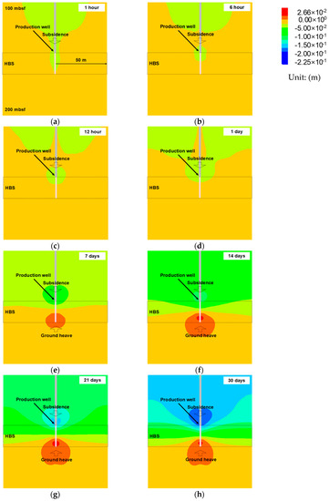
Figure 10.
Distribution of z-axis displacement with production period: (a) after 1 hour; (b) after 6 hours; (c) after 12 hours; (d) after 1 day; (e) after 7 days; (f) after 14 days; (g) after 21 days; (h) after 30 days.
Distribution of confining stress under depressurization is shown in Figure 11. The development of the confining stress distribution with production period shows a rhomboid shape slightly shifted downward. Based on the previous results of lateral and vertical displacements, this shape can be explained. A rhomboid shape is induced by the distribution of lateral displacement, which shows maximum displacement at the middle of HBS. In addition, the reason for slightly shifting the maximum value is because of imbalance between the subsidence and ground heave (i.e., the neutral point appears slightly below from the middle). From these results, it is inferred that compressive stresses are generated on the wellbore at HBS, and the maximum axial compressive stress will occur at the point where displacement is zero (i.e., a point slightly below the middle of HBS). For reasons similar to those mentioned above, the maximum confining stress was about 11.4 MPa at slightly below the middle of HBS as shown in Figure 11h. Through the stability analysis of HBS during gas hydrate production, we can predict that the production wellbore at HBS will be subjected to axial compressive stress according to the ground behavior. In addition, it was confirmed that the coupling stiffness model considering confining stress should be applied with depth for accurate stability analysis of the wellbore.
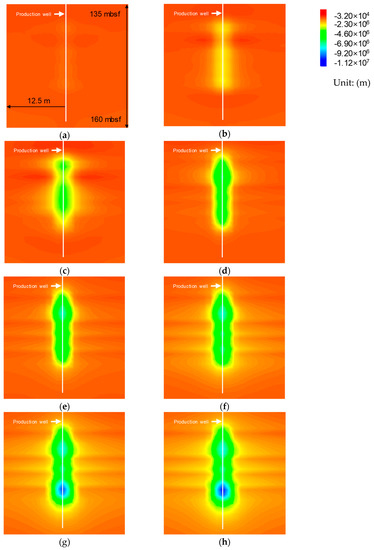
Figure 11.
Distribution of confining stress with production period: (a) after 1 hour; (b) after 6 hours; (c) after 12 hours; (d) after 1 day; (e) after 7 days; (f) after 14 days; (g) after 21 days; (h) after 30 days.
3.2. Effects of Coupling Stiffness and Confining Stress on Axial Stress of Wellbore
The shear and normal coupling stiffness at the interface are widely used to simulate the interface behavior in numerical analysis [35,38,39,50]. The shear and normal coupling stiffness act as the coefficient of friction of interface between the wellbore and sediments. Typical values of the shear and normal stiffness for rock joints range from roughly 10 to 100 MPa/m for joints with soft clay in-filling [48,51,52]. According to the roughness differences between steel plate and rock, the experimental value obtained in this study is the value for the interface between soil and steel plate, which can be considered to be an appropriate value based on the aforementioned range (i.e., 10 to 100 MPa/m). Additionally, we confirmed that the shear and normal coupling stiffness vary with the confining stress (see Section 2.2.3). This section describes the effects of coupling stiffness and confining stress on axial stress of wellbore.
3.2.1. Parametric Analysis
The effective stress increases with decreasing pore pressure during depressurization. For this reason, the ground subsidence of HBS take places and induces the axial stress of the wellbore by pulling the wellbore down during production. A parametric study was performed to determine the effects of the shear and normal coupling stiffness on the stability of wellbore. Cases were defined based on the direct shear test data with confining stress of 600 kPa and consolidation test data with confining stress of 1500 kPa (case I). The effects of confining stress have not been considered in cases I to IV (using the FLAC3D model). Additionally, case V (using the new model described in Section 2.2.3, i.e., the applied coupling stiffness model considering confining stress) was defined to determine the effects of confining stress on axial stress of the wellbore. The applied cases are summarized in Table 3.
Table 3.
Comparison of cases for parametric analyses.
3.2.2. Results of Parametric Study
The results of the parametric study are shown in Figure 12. The production period for parametric analyses is 14 days. The distribution of axial stress on the wellbore for case I is shown in Figure 12a. As shown in Figure 12a, the compressive and tensile stresses on the wellbore are developed due to the ground subsidence. The distribution of axial stress on the wellbore in other cases also showed a similar trend to case I. The maximum compressive and tensile stress of each case are shown in Figure 12b. The yield strength of the production wellbore (9 5/8” casing) is 454.8 MPa in this study. The compressive axial stress of case I, II and V (Figure 12b) exceed the yield strength of the wellbore located at the screen parts. By contrast, results of case III and IV show compressive stresses of the wellbore lower than the yield strength and the tensile stresses are similar for all cases.
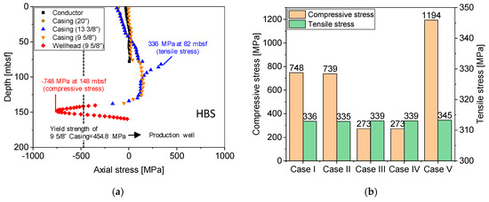
Figure 12.
Distribution of axial stresses with depth (non-consideration of the slippage at the interface): (a) Distribution of axial stress with depth for case I; (b) comparison of the maximum compressive and tensile stress.
The effect of normal coupling stiffness on axial stress can be confirmed through the comparison between case I and II or case III and IV. Cases I has a normal stiffness 10 times higher than those of case II. The results show that the compressive and tensile stress increased about 1.2% (i.e., from 739 to 748 MPa) and 0.3% (i.e., from 335 to 336 MPa), respectively, while normal stress increased 10 times. On the other hand, case III has a normal stiffness twice as high as those of case IV, but show almost no difference in axial stresses. The effect of shear coupling stiffness can be confirmed by the comparison between case I and IV. These cases have 10 times difference in the shear coupling stiffness, and show that the maximum compressive stress significantly increased about 174% (i.e., from 273 to 748 MPa). From the above comparisons, it can be concluded that the shear coupling stiffness significantly affects the development of axial stress of the wellbore, while the normal coupling stiffness has little effect.
In addition, the effect of the confining stress on the axial stress development of the wellbore can be explained in case V. The maximum axial compressive stress, 1194.6 MPa, of case V was about 2.6 times greater than the yield strength of the wellbore and significantly greater than those of other cases. The considerably large development of the maximum axial compressive stress compared to other cases is due to the large shear and coupling stiffness according to the increase of confining stress. During the 14-day period of gas production, the pore pressure decreased to 9 MPa and consequently the confining stress increased until about 7.6 MPa. After 14 days of gas production, relatively large shear and normal coupling stiffness (319.8 and 239.4 MPa, respectively) were derived by the coupling stiffness models considering the confining stress. This large shear and normal coupling stiffness increased axial stress on the wellbore. From this result, it is concluded that the consideration of confining stress largely affects the development of axial stress on the wellbore. Therefore, the variation of confining stress should be considered in coupling stiffness models for accurate analysis.
3.3. Effects of Slippage at the Interface
As described in Section 3.1, the confining stress increases during gas hydrate production. Relatively high maximum compressive stress was derived in Section 3.2 due to non-application of slippage phenomena. In this section, stability analysis was performed by considering the slippage phenomenon according to the Coulomb stress–strain criterion (see Section 2.3). Development of compressive stress with the production period is shown in Figure 13a. The pore pressure (i.e., bottom hole pressure) near the screen part decreased from the initial state, 23.5 MPa, to target pressure, 9 MPa. The depressurization rate was 0.5 MPa/h in this study. After 29 hours of gas production, the bottom hole pressure was reduced to 9 MPa and this pressure spreads out of the production wellbore. Under the influence of changes in pore pressure, the confining stress also rapidly increased in the initial state. The compressive stress sharply increased in the depressurization period and converged to a certain value (334.9 MPa for this study). The shape of the development of axial compressive stress of the wellbore was similar to the Coulomb stress-strain curve (Figure 6).
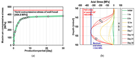
Figure 13.
Results of stability analysis considering the coupling stiffness models: (a) Development of the maximum axial stresses with production period; (b) distribution of axial stress with depth.
Distributions of axial stress with depth of the wellbore under depressurization are shown in Figure 13b. The maximum axial compressive stress converged to 334.9 MPa from 14 days after the beginning of depressurization. The generated maximum axial stress is about 74% of the yield strength of the wellbore, 454.9 MPa. This means that the production well will be stable until 30 days after the start of production. The maximum compressive stress converges to a constant value, and the convergence range gradually spreads to the whole range of the production wellbore. This is because the coupling stiffness applied differently with the depth of wellbore, and is considered to be zero after the slippage phenomena (see Section 2.4). Similar to the geotechnical behaviors of the previous section, the maximum axial compressive stress has been observed from about 153 mbsf in which the neutral point is described in Section 3.1.
4. Discussion
4.1. Comparison of the Models
This section suggests a suitable method for stability analysis of the wellbore based on the results of the present study. The axial stress on the wellbore was largely affected by the coupling stiffness and, as shown in the distribution of confining stress (see Figure 11), the confining stress varies with the depth of the wellbore. From the results of the direct shear test, it was revealed that the coupling stiffness changes with confining stress. However, the existing model of the shear and normal coupling stiffness in FLAC3D is the function of the shear and bulk modulus without consideration of the confining stress. Therefore, it is difficult to obtain accurate stability analysis results using the existing model in FLAC3D. This study suggests that the stability analysis for the wellbore during gas hydrate production has to consider the coupling stiffness differently with confining stress according to the depth. Parametric studies have been conducted to investigate the effect of coupling stiffness change according to the depth on the development of the axial stress on the wellbore to verify the proposed stability analysis method.
The previous section described the effects of coupling stiffness and geotechnical behavior on development of axial stress. In this section, parametric analysis was carried out to understand the effects of coupling stiffness model and slippage at the interface. Assigned cases for the parametric analysis are summarized in Table 4.
Table 4.
Comparison of cases for parametric analysis.
As a control case, Case A did not apply the coupling stiffness model and the slippage at the interface. Case B applied the existing FLAC3D model, which is the function of the shear and bulk modulus without consideration of confining stress, as a coupling stiffness model. Case C applied the linear regression models derived from this study, and does not consider the slippage at the interface. Case D applied the linear regression model and also considered the slippage at the interface. The production period was set to be 14 days for all cases.
4.2. Comparison of Results According to Model Application
Results according to model application are shown in Figure 14a and comparison of the maximum compressive and tensile stresses of each case are shown in Figure 14b. Case A, which does not consider the coupling stiffness, showed almost zero axial stress on the wellbore because the transferred stress from the sediments to the wellbore was too small. Cases B and C yielded maximum axial compressive stresses of 520.4 MPa and 1194.6 MPa, respectively. This difference of the maximum compressive stress is due to the difference of coupling stiffness. The shear coupling stiffness of case C (339 MPa/m) is about 3.72 times larger than that of Case B (91 MPa/m for sand sediment) at the completion of depressurization (see Figure 5). As a result, the maximum compressive stresses of C is 2.3 times higher than those of case B. This result tends to be similar to the results of parametric studies to derive the effects of coupling stiffness (see Section 3.2). The maximum compressive stresses of both Cases B and C exceeded the yield strength of 9 5/8” casing, 454.8 MPa. Unlike the results of Cases B and C, Case D shows that the maximum axial compressive stress, 334.9 MPa, of the wellbore was lower than the yield strength of the 9 5/8” casing.
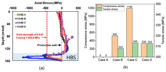
Figure 14.
Results of parametric analyses: (a) Distribution of axial stress; (b) the maximum axial stresses.
Because the coupling stiffness acts as a spring constant at the interface between the wellbore and soil sediments in the numerical analysis, the large coupling stiffness induces the large axial stress according to the ground subsidence. Therefore, it is deduced that the case for non-consideration of the slippage phenomena over-estimates axial stress. From the results of parametric study, it is revealed that the proposed method, which considers the coupling stiffness differently with depth, can accurately simulate the stability of the wellbore during the gas hydrate production.
5. Conclusions
The aim of the present study was to evaluate the stability of a production wellbore under the depressurization method for gas hydrate production from hydrate bearing sediments. In order to evaluate the stability of the wellbore, it is essential to consider the interface behavior between the wellbore and hydrate bearing sediments. In this paper, an algorithm for wellbore stability analysis was suggested. The effects of the shear and normal coupling stiffness were investigated and coupling stiffness models, which considered confining stress and slippage phenomena, were suggested and applied to the algorithm. The key findings from this study are as follows:
- The shear and normal coupling stiffness have to be considered to simulate the interface between the wellbore and the ground. From the parametric analysis relating coupling stiffness to wellbore stability, shear coupling stiffness has a significant effect on the development of axial stress of the wellbore while normal coupling stiffness does not affect the development of axial stress on the wellbore.
- The shear and normal coupling stiffness are the function of confining stress. This study derived a coupling stiffness model considering confining stress by performing the direct shear test and consolidation test.
- The shear coupling stiffness has to be considered differently from the depth of the wellbore to estimate the actual development of axial stress on the wellbore.
- The compressive stress is induced at the wellbore due to the subsidence and heave of the ground.
- As the effective stress with depressurization for gas hydrate production increases, slippage occurs between the wellbore and the ground because of shear failure. After shear failure, additional axial stress on the wellbore is not developed. For this reason, the maximum generated axial stress converges to a whole range during gas hydrate production.
- Preferentially, the maximum axial stress occurs at the neutral point where displacement is zero, and gradually converges to the whole range of the wellbore. The final conclusion based on the key findings is that the coupling stiffness has to be considered differently from the depth of the wellbore, and the slippage phenomena also has to be considered to performed accurate stability analysis.
This study contains limitation and the authors suggest further work. In this study, the coupling stiffness models are valid only for Ulleung basin because the models were derived from the experimental results using Ulleung basin sediment. In order to improve the applicability of the models, it is necessary to develop them including factors (e.g., bulk and shear modulus) that can consider the characteristics of the soil type.
Author Contributions
Conceptualization, G.-C.C. and J.-T.K.; numerical analysis, J.-T.K. and A.-R.K.; experiment, C.-W.K.; analysis of data, J.-T.K. and A.-R.K.; writing—original draft preparation, J.-T.K.; writing—review and editing, A.-R.K. and G.-C.C.; supervision, G.-C.C.; project administration, J.Y.L.
Funding
This research was supported by the Ministry of Trade, Industry, and Energy (MOTIE) through the Project “Gas Hydrate Exploration and Production Study (18-1143)” under the management of the Gas Hydrate Research and Development Organization (GHDO) of Korea and the Korea Institute of Geoscience and Mineral Resources (KIGAM) and supported by the National Research Foundation of Korea (NRF) grant funded by the Korea government (MSIT) (No. 2018R1C1B6008417).
Conflicts of Interest
The authors declare no conflict of interest.
References
- Yin, Z.; Khurana, M.; Tan, H.K.; Linga, P. A review of gas hydrate growth kinetic models. Chem. Eng. J. 2018, 342, 9–29. [Google Scholar] [CrossRef]
- Chong, Z.R.; Yang, S.H.B.; Babu, P.; Linga, P.; Li, X.-S. Review of natural gas hydrates as an energy resource: Prospects and challenges. Appl. Energy 2016, 162, 1633–1652. [Google Scholar] [CrossRef]
- Sloan, E.D. Fundamental principles and applications of natural gas hydrates. Nature 2003, 426, 353. [Google Scholar] [CrossRef] [PubMed]
- Rossi, F.; Gambelli, A.M.; Sharma, D.K.; Castellani, B.; Nicolini, A.; Castaldi, M.J. Experiments on methane hydrates formation in seabed deposits and gas recovery adopting carbon dioxide replacement strategies. Appl. Therm. Eng. 2019, 148, 371–381. [Google Scholar] [CrossRef]
- Lu, H.; Seo, Y.-T.; Lee, J.-W.; Moudrakovski, I.; Ripmeester, J.A.; Chapman, N.R.; Coffin, R.B.; Gardner, G.; Pohlman, J. Complex gas hydrate from the Cascadia margin. Nature 2007, 445, 303. [Google Scholar] [CrossRef]
- Makogon, Y.F. Natural gas hydrates—A promising source of energy. J. Nat. Gas. Sci. Eng. 2010, 2, 49–59. [Google Scholar] [CrossRef]
- Park, K.-P.; Bahk, J.-J.; Kwon, Y.; Kim, G.Y.; Riedel, M.; Holland, M.; Schultheiss, P.; Rose, K. Korean national Program expedition confirms rich gas hydrate deposit in the Ulleung Basin, East Sea. Fire Ice Methane Hydrate Newsl. 2008, 8, 6–9. [Google Scholar]
- Kim, G.Y.; Yi, B.Y.; Yoo, D.G.; Ryu, B.J.; Riedel, M. Evidence of gas hydrate from downhole logging data in the Ulleung Basin, East Sea. Mar. Pet. Geol. 2011, 28, 1979–1985. [Google Scholar] [CrossRef]
- Ryu, B.-J.; Collett, T.S.; Riedel, M.; Kim, G.Y.; Chun, J.-H.; Bahk, J.-J.; Lee, J.Y.; Kim, J.-H.; Yoo, D.-G. Scientific results of the second gas hydrate drilling expedition in the Ulleung basin (UBGH2). Mar. Pet. Geol. 2013, 47, 1–20. [Google Scholar] [CrossRef]
- Kang, N.; Yoo, D.; Yi, B.; Bahk, J.; Ryu, B. Resources Assessment of Gas Hydrate in the Ulleung Basin, Offshore Korea. In Proceedings of the AGU Fall Meeting Abstracts, San Francisco, CA, USA, 3–7 December 2012. [Google Scholar]
- Lee, G.H.; Bo, Y.Y.; Yoo, D.G.; Ryu, B.J.; Kim, H.J. Estimation of the gas-hydrate resource volume in a small area of the Ulleung Basin, East Sea using seismic inversion and multi-attribute transform techniques. Mar. Pet. Geol. 2013, 47, 291–302. [Google Scholar] [CrossRef]
- Riedel, M.; Bahk, J.-J.; Kim, H.-S.; Scholz, N.; Yoo, D.; Kim, W.-S.; Ryu, B.-J.; Lee, S. Seismic facies analyses as aid in regional gas hydrate assessments. Part-II: Prediction of reservoir properties, gas hydrate petroleum system analysis, and Monte Carlo simulation. Mar. Pet. Geol. 2013, 47, 269–290. [Google Scholar] [CrossRef]
- Bo, Y.Y.; Lee, G.H.; Kang, N.K.; Yoo, D.G.; Lee, J.Y. Deterministic estimation of gas-hydrate resource volume in a small area of the Ulleung Basin, East Sea (Japan Sea) from rock physics modeling and pre-stack inversion. Mar. Pet. Geol. 2018, 92, 597–608. [Google Scholar]
- Holder, G.; Kamath, V.; Godbole, S. The potential of natural gas hydrates as an energy resource. Annu. Rev. Energy 1984, 9, 427–445. [Google Scholar] [CrossRef]
- Collett, T.; Bahk, J.-J.; Baker, R.; Boswell, R.; Divins, D.; Frye, M.; Goldberg, D.; Husebø, J.; Koh, C.; Malone, M. Methane Hydrates in Nature Current Knowledge and Challenges. J. Chem. Eng. Data 2014, 60, 319–329. [Google Scholar] [CrossRef]
- Dallimore, S.; Collett, T. Summary and implications of the Mallik 2002 gas hydrate production research well program. Sci. Results Mallik 2005, 585, 1–36. [Google Scholar]
- Yamamoto, K.; Terao, Y.; Fujii, T.; Ikawa, T.; Seki, M.; Matsuzawa, M.; Kanno, T. Operational overview of the first offshore production test of methane hydrates in the Eastern Nankai Trough. In Proceedings of the Offshore Technology Conference, Houston, TX, USA, 5–8 May 2014. [Google Scholar]
- Moridis, G.J.; Collett, T.S.; Boswell, R.; Hancock, S.; Rutqvist, J.; Santamarina, C.; Kneafsey, T.; Reagan, M.T.; Pooladi-Darvish, M.; Kowalsky, M. Gas hydrates as a potential energy source: State of knowledge and challenges. In Advanced Biofuels and Bioproducts; Springer: Berlin, Germany, 2013; pp. 977–1033. [Google Scholar]
- Moridis, G.J. TOUGH+ HYDRATE v1. 2 User’s Manual: A Code for the Simulation of System Behavior in Hydrate-Bearing Geologic Media; University of California: Berkeley, CA, USA, 2012. [Google Scholar]
- Moridis, G.; Kowalsky, M.; Pruess, K. HydrateResSim Users Manual: A Numerical Simulator for Modeling the Behavior of Hydrates in Geologic Media; Lawrence Berkeley National Laboratory: Berkeley, CA, USA, 2005. [Google Scholar]
- Kurihara, M.; Ouchi, H.; Masuda, Y.; Narita, H.; Okada, Y. Assessment of Gas Productivity of Natural Methane Hydrates Using MH21 Reservoir Simulator; Natural Gas Hydrates/Energy Resource Potential Associated Geologic Hazards: Vancouver, BC, Canada, 2004. [Google Scholar]
- White, M. Impact of kinetics on the injectivity of liquid CO2 into Arctic hydrates. In Proceedings of the OTC Arctic Offshore Technology Conference, Houston, TX, USA, 7 February 2011. [Google Scholar]
- Kim, A. THM Coupled Numerical Analysis of Gas Production from Methane Hydrate Deposits in the Ulleung Basin in Korea. Ph.D. Thesis, Korea Advanced Institute of Science and Technology (KAIST), Daejeon, Korea, 2016. [Google Scholar]
- Kim, A.-R.; Kim, J.-T.; Cho, G.-C.; Lee, J.Y. Methane Production From Marine Gas Hydrate Deposits in Korea: Thermal-Hydraulic-Mechanical Simulation on Production Wellbore Stability. J. Geophys. Res. Solid Earth 2018, 123, 9555–9569. [Google Scholar] [CrossRef]
- Masuda, Y. Modeling and experimental studies on dissociation of methane gas hydrates in Berea sandstone cores. In Proceedings of the Third International Gas Hydrate Conference, Salt Lake City, UT, USA, 18–22 July 1999. [Google Scholar]
- Kim, A.-R.; Kim, H.-S.; Cho, G.-C.; Lee, J.Y. Estimation of model parameters and properties for numerical simulation on geomechanical stability of gas hydrate production in the Ulleung Basin, East Sea, Korea. Quat. Int. 2017, 459, 55–68. [Google Scholar] [CrossRef]
- Zheng, R.; Li, S.; Li, Q.; Li, X. Study on the relations between controlling mechanisms and dissociation front of gas hydrate reservoirs. Appl. Energy 2018, 215, 405–415. [Google Scholar] [CrossRef]
- Zheng, R.; Li, S.; Li, X. Sensitivity analysis of hydrate dissociation front conditioned to depressurization and wellbore heating. Mar. Pet. Geol. 2018, 91, 631–638. [Google Scholar] [CrossRef]
- Su, Z.; Cao, Y.; Wu, N.; He, Y. Numerical analysis on gas production efficiency from hydrate deposits by thermal stimulation: Application to the Shenhu Area, south China sea. Energies 2011, 4, 294–313. [Google Scholar] [CrossRef]
- Ruan, X.; Song, Y.; Zhao, J.; Liang, H.; Yang, M.; Li, Y. Numerical simulation of methane production from hydrates induced by different depressurizing approaches. Energies 2012, 5, 438–458. [Google Scholar] [CrossRef]
- Sun, Z.; Xin, Y.; Sun, Q.; Ma, R.; Zhang, J.; Lv, S.; Cai, M.; Wang, H. Numerical simulation of the depressurization process of a natural gas hydrate reservoir: An attempt at optimization of field operational factors with multiple wells in a real 3D geological model. Energies 2016, 9, 714. [Google Scholar] [CrossRef]
- Wang, Y.; Feng, J.-C.; Li, X.-S.; Zhang, Y.; Li, G. Evaluation of gas production from marine hydrate deposits at the GMGS2-Site 8, Pearl river Mouth Basin, South China Sea. Energies 2016, 9, 222. [Google Scholar] [CrossRef]
- Ruan, X.; Li, X.-S.; Xu, C.-G. Numerical Investigation of the Production Behavior of Methane Hydrates under Depressurization Conditions Combined with Well-Wall Heating. Energies 2017, 10, 161. [Google Scholar] [CrossRef]
- Feng, Y.; Chen, L.; Suzuki, A.; Kogawa, T.; Okajima, J.; Komiya, A.; Maruyama, S. Numerical analysis of gas production from layered methane hydrate reservoirs by depressurization. Energy 2019, 166, 1106–1119. [Google Scholar] [CrossRef]
- Jeong, S.; Lee, J.; Lee, C.J. Slip effect at the pile-soil interface on dragload. Comput. Geotech. 2004, 31, 115–126. [Google Scholar] [CrossRef]
- Chen, R.; Zhou, W.; Chen, Y. Influences of soil consolidation and pile load on the development of negative skin friction of a pile. Comput. Geotech. 2009, 36, 1265–1271. [Google Scholar] [CrossRef]
- Abdrabbo, F.M.; Ali, N.A. Behaviour of single pile in consolidating soil. Alex. Eng. J. 2015, 54, 481–495. [Google Scholar] [CrossRef]
- Itasca, F.D. Fast lagrangian analysis of continua in 3 dimensions; Itasca Consulting Group Inc.: Minneapolis, MN, USA, 2005. [Google Scholar]
- Häggblad, B.; Nordgren, G. Modelling nonlinear soil-structure interaction using interface elements, elastic-plastic soil elements and absorbing infinite elements. Comput. Struct. 1987, 26, 307–324. [Google Scholar] [CrossRef]
- Kim, J.; Moridis, G.J.; Rutqvist, J. Coupled flow and geomechanical analysis for gas production in the Prudhoe Bay Unit L-106 well Unit C gas hydrate deposit in Alaska. J. Pet. Sci. Eng. 2012, 92, 143–157. [Google Scholar] [CrossRef]
- Rutqvist, J.; Moridis, G.; Grover, T.; Silpngarmlert, S.; Collett, T.; Holdich, S. Coupled multiphase fluid flow and wellbore stability analysis associated with gas production from oceanic hydrate-bearing sediments. J. Pet. Sci. Eng. 2012, 92, 65–81. [Google Scholar] [CrossRef]
- Kamath, V.A. Study of Heat Transfer Characteristics During Dissociation of Gas Hydrates in Porous Media; Pittsburgh University: Pittsburgh, PA, USA, 1984. [Google Scholar]
- Clarke, M.; Bishnoi, P.R. Determination of the activation energy and intrinsic rate constant of methane gas hydrate decomposition. Can. J. Chem. Eng. 2001, 79, 143–147. [Google Scholar] [CrossRef]
- Darcy, H.P.G. Les Fontaines Publiques de la Ville de Dijon. Exposition et Application des Principes à Suivre et des Formules à Employer dans les Questions de Distribution d’eau; Dalamont, V., Ed.; Libraire des Corps Imperiaux des Ponts et Chaussees et des Mines: Paris, France, 1856. [Google Scholar]
- Van Genuchten, M.T. A closed-form equation for predicting the hydraulic conductivity of unsaturated soils 1. Soil Sci. Soc. Am. J. 1980, 44, 892–898. [Google Scholar] [CrossRef]
- Zeghal, M.; Edil, T.B. Soil structure interaction analysis: Modeling the interface. Can. Geotech. J. 2002, 39, 620–628. [Google Scholar] [CrossRef]
- Salemi, A.; Esmaeili, M.; Sereshki, F. Normal and shear resistance of longitudinal contact surfaces of segmental tunnel linings. Int. J. Rock Mech. Min. Sci. 2015, 77, 328–338. [Google Scholar] [CrossRef]
- Rosso, R.S. A comparison of joint stiffness measurements in direct shear, triaxial compression, and In Situ. Int. J. Rock Mech. Min. Sci. Geomech. Abstr. 1976, 13, 167–172. [Google Scholar] [CrossRef]
- Li, W.; Bai, J.; Cheng, J.; Peng, S.; Liu, H. Determination of coal–rock interface strength by laboratory direct shear tests under constant normal load. Int. J. Rock Mech. Min. Sci. 2015, 77, 60–67. [Google Scholar] [CrossRef]
- Jeong, S.; Cho, J. Proposed nonlinear 3-D analytical method for piled raft foundations. Comput. Geotech. 2014, 59, 112–126. [Google Scholar] [CrossRef]
- Kulhawy, F.H. Stress deformation properties of rock and rock discontinuities. Eng. Geol. 1975, 9, 327–350. [Google Scholar] [CrossRef]
- Bandis, S.C.; Lumsden, A.C.; Barton, N.R. Fundamentals of rock joint deformation. Int. J. Rock Mech. Min. Sci. Geomech. Abstr. 1983, 20, 249–268. [Google Scholar] [CrossRef]


© 2019 by the authors. Licensee MDPI, Basel, Switzerland. This article is an open access article distributed under the terms and conditions of the Creative Commons Attribution (CC BY) license (http://creativecommons.org/licenses/by/4.0/).