Article

Research on Intelligent Predictive AGC of a Thermal Power Unit Based on Control Performance Standards

School of Automation Engineering, Shanghai University of Electric Power, Shanghai 200090, China
*
Author to whom correspondence should be addressed.
Energies 2019, 12(21), 4073; https://doi.org/10.3390/en12214073
Submission received: 5 July 2019 / Revised: 12 October 2019 / Accepted: 23 October 2019 / Published: 25 October 2019

Abstract

:
In order to satisfy the growing demands of control performance and operation efficiency in the automatic generation control (AGC) system of a grid, a novel, intelligent predictive controller, combined with predictive control and neural network ideas, is proposed and applied to the AGC systems of thermal power units. This paper proposes a Bayesian neural network identification model for typical ultra-supercritical thermal power units, which was found to be accurate and can be used as a simulation model. Based on the model, this paper develops an intelligent predictive control for the AGC of thermal power units, which improves unit load operation and constitutes a novel, closed-loop AGC structure based on online control performance standard (CPS) evaluations. Intelligent predictive control is mainly improved because the neural network rolling optimization model replaces the traditional rolling optimization model in the rolling optimization module. The simulation results indicate that the intelligent predictive controller developed in the two-area interconnected power grid under CPS can, on the one hand, improve the load tracking performance of AGC thermal power units, and, on the other hand, the controller has strong robustness. Whether the system parameters change considerably or the AGC has different grid disturbances, the new type of the loop AGC system can still sufficiently meet the control requirements of the power grid.

1. Introduction

With the increasing complexity and scale of modern power system structures, more and more uncertain disturbances have brought tremendous new challenges to power grid security. It has become a pressing issue to ensure the safe and stable operation of the power grid [1,2]. Automatic generation control (AGC) is an advanced technique used in power grid dispatching centers. Its core task is to establish closed-loop control between the power grid dispatching energy management system (EMS) and the coordinated control system (CCS) of different thermal power generation units to maintain power grid frequency within an allowable range. Therefore, AGC has been a hot spot in power system research [3,4,5].
In previous research on AGC control systems, it has been difficult to establish a more accurate mathematical model because there are relatively complex nonlinear and time-varying parameters and structures in the existing interconnected power grid AGC system. Currently, traditional proportional-integral-derivative (PID) controllers are used in Chinese AGC control strategies because they have simple structures and are easy to implement. However, serious overshooting phenomena are often detected because of the fixed parameters of the controllers. In recent years, in order to cover the shortage of traditional AGC PID controllers, many scholars have tried to apply intelligent control strategies to AGC systems, which have played a guiding role in AGC research [6,7,8]. Scholars have applied advanced control methods including genetic algorithms in [9], fuzzy predictive control in [10], and the combination of various control methods [11] in the AGC system to improve development of the AGC system to some degree. Nanda et al. [12] proposed using the genetic algorithm (GA) to optimize control of the AGC system. However, this method has some shortcomings, as GA only carries out crossover and mutation operations, and it is likely to fall into local optimum or premature convergence. This has resulted in a dramatic reduction in the efficiency and searchability of the algorithm. Gozde and Taplamacioglu [13] developed a gain-scheduling proportional-integral (PI) controller for a dead zone, nonlinear AGC system. The authors used the craziness-based particle swarm optimization algorithm to minimize the standard error and solution time of different objective functions. Rabindra Kumar Sahu et al. [14] changed the controller design problem into a controller optimization problem for automatic generation control (AGC) of multi-area power systems with diverse energy sources. The proposed teaching learning based optimization (TLBO) algorithm was employed to optimize the parameters of the PID controller, and the superiority of the proposed TLBO controller has been demonstrated by simulation comparison experiments.
Appropriate models serve for excellent control algorithms. As one of the intelligent algorithms, model predictive control (MPC) is advantageous because of its unique model prediction, rolling optimization, and feedback correction structure [15,16]. An MPC algorithm was presented to control coal convey systems in a coal-fired power plant [17]. Nevertheless, control performance decreased with an increase in the order of state–space models, which is the shortcoming of MPC [18]. In China, the majority of power generation units in the AGC system are thermal power units. Therefore, the control quality of these thermal power units can seriously affect the control quality of the AGC system. In the performance assessment of thermal power units, primary frequency assessments of most provincial power grids in China follow “two rules”, which assess primary frequency modulation and daily generation plan. The North American Electric Reliability Council (NERC) proposes an improved control performance standard (CPS) [10], which incorporates quantitative statistical analyses of area control error (ACE) and frequency deviation over a specified time period to ensure safe operation of the power system and to take into account the interests of different control areas. Under the guidance of this evaluation method, it can effectively reduce the number of operations of the AGC unit. This evolution method can prolong the life of the units to some extent; therefore, the CPS can accurately evaluate the control performance of the unit control system.
The coordination control system (CCS) of power plants plays an important role in the realization of an AGC system whose main task is to balance the supply and demand between the output power and demands of the grid [19]. Thus, AGC can only be put into operation when the CCS of the generator units is in a normal and stable operation. CCS is the core of ultra-supercritical units, and its safe and stable operation is also one of the hotspots in current research. The nonlinearity, coupling, and uncertainty of CCSs are often neglected by traditional modelling methods [20,21,22,23]. In order to solve this problem, many intelligent algorithms have been proposed such as fuzzy identification [24,25], support vector machines [26], neural networks [27,28], and so on. Among them, establishment of a neural network model can adequately solve the problem of nonlinear samples, but the neural network model is still problematic in finding the local optimum of the algorithm. Ravindra Singh et al. [29] proposed a Bayesian algorithm based on statistical concepts, which transformed the weight optimization problem into solving the minimum regularization error so as to avoid falling into the local optimum. The Bayesian neural network is a black-box identification method that has no prior knowledge of the system mechanisms.
From the above literature survey, there are few controller designs based on CPS in the current field of AGC research, and there is still room for further improvement in the optimization of controller parameters. However, in simulation experiments of AGC, most CCSs are expressed only by transfer functions, so the nonlinear, coupling, and uncertainty of CCS systems are not fully considered. For this purpose, this paper proposed a novel identification method and tested it.
Intelligent predictive AGC of thermal power units based on control performance standards are used to improve the energy-saving ability and operation efficiency of AGC and enhance the adaptability of interconnected power grids to CPS. To specify, an intelligent predictive controller for an AGC system is designed by combining a black-box model, trained by actual historical data from a power plant, with intelligent control and classical predictive control ideas. It avoids the error between the mathematical model of the AGC system and real data, enables a more realistic simulation, and enhances the anti-disturbance ability of the system. At first, a Bayesian neural network model for typical ultra-supercritical thermal power units was developed. Through K-fold cross-validation experiments and comparative experiments of fuzzy algorithm [25] modeling, the Bayesian neural network proved to be a more accurate simulation model. Secondly, an intelligent predictive control for thermal power units was developed, which improved unit load operations and formed a novel, closed-loop AGC structure based on online control performance standard evaluations. Finally, the experiment proved that the intelligent predictive controller developed in the two-area interconnected power grid under CPS can, on the one hand, improve the load tracking performance of thermal power units under AGC rules, and, on the other hand, the controller has strong robustness. Whether the system parameters change considerably, or different grid disturbances are added, the new type of the loop AGC system can still meet the control requirements of the power grid very well.

2. AGC System Structure and CPS

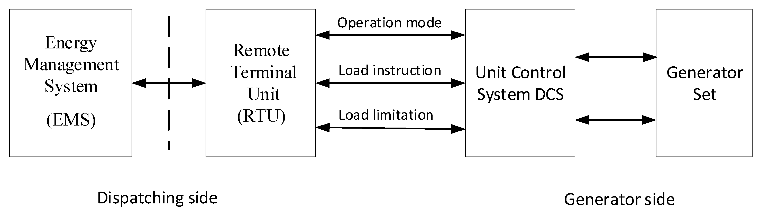
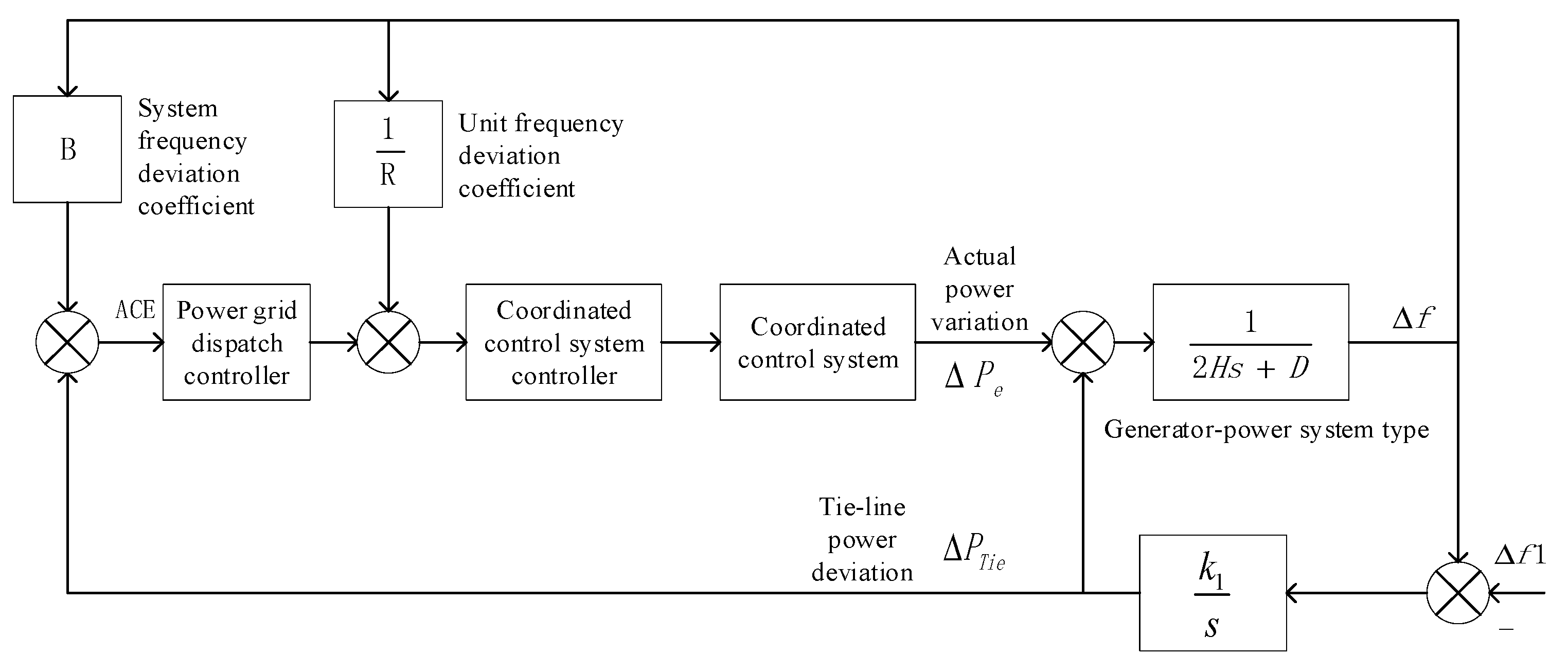
2.1. AGC System Structure

AGC refers to the load output instructions by the CCS of power plants according to the calculation results of the energy management system (EMS) of the power grid dispatching center, which can automatically adjust the output of each generating unit to maintain the frequency of the power grid and the exchange power of regional tie lines within the prescribed range [30,31]. AGC can be divided into two levels: the dispatching side (decision control layer) and the power generation unit side (instruction execution layer). The AGC mainly has three parts, which are EMS, remote terminal unit (RTU), and CCS of the distributed control system (DCS) in power plants, and its structure is shown in Figure 1.
The CCS of power plants plays an important role in the realization of the AGC system. AGC can only be put into operation when the CCS of the generator units are in a normal and stable operation. Only one typical CCS of a thermal power unit is included in the unit AGC system in this paper to show the relationship between AGC and CCS clearly. The system structure model [32,33] is shown in Figure 2. The dispatching controller adopts a PI controller [34]; the CCS controller adopts more advanced predictive control; the CCS model is identified by the power plant data; the generator power system model is derived from the generator energy balance equation and other related equations. H represents the value of the inertia coefficient of the generator. After multiple tests, the value of H was set to 11.845. D is the per unit value of load regulation, that is, the change in the percentage of load when the system frequency changes by one percentage point. Because of the different characteristics and proportions of the load, the value of D will change correspondingly. In practice, D usually takes a value of one to three, indicating that when the frequency changes by one percentage point, the active power of the load will change by one to three percentage points; the system and unit frequency deviation coefficients are constants.

2.2. CPS

The CPS evaluation standard that was proposed by NERC in 1996 [35] mainly evaluates the control performance of the system by quantitative statistical analysis of the product of the regional control deviation, ACE, and the frequency deviation ( Δ f ) of the system in a certain period. Unlike previous control performance evaluation methods, which measure the AGC system with a single frequency deviation and the absolute size of the ACE system area with control deviation, CPS uses the product of the two as a reference, and ACE is defined as follows [36]:
A C E = 10 B Δ f + Δ P = 10 B ( f A f s ) + ( P A P s ) .
In Formula (1), f A represents the actual frequency of the power grid in Hz; f S is the planned frequency of the power grid in Hz; and P A is the actual switching frequency in MW, which is the actual power algebra sum of all external tie lines in the region. P S is the planned exchange power in MW, and B is the frequency deviation coefficient of the power grid for all external tie lines in the region. The unit is MW/0.1 Hz with negative values.
From Formula (1), it can be found that when ACE is positive, the frequency will rise if the region overruns at this time; when ACE is negative, the frequency will decrease when ACE is less frequent in this region. Therefore, new A C E × Δ f criteria can then be introduced: When A C E × Δ f > 0 , the frequency recovery of the system is unfavorable, requiring AGC regulation; when A C E × Δ f < 0 , the frequency recovery of the system is favorable, and AGC will not be adjusted.
CPSs include CPS1 and CPS2. CPS1 evaluates over a month or a year, and the system area control deviation ACE satisfies Equation (2) [36]:
A C E 1 min 10 × B × Δ f ε 1 min 2 .
In the formula, ε 1 min represents the root mean square of the one-minute average deviation between the actual frequency and the rated frequency of the system in a year or a month, and it is a constant.
The calculation formula of the control index CPS1 is represented by Equation (3) [36]:
C P S 1 = ( 2 C F ) × 100 % .
CF is the coordination factor in Formula (4), and its calculation formula is expressed as follows [36], where B is taken as 20 MW/0.1 Hz:
C F = a v g ( A C E × Δ f 10 × B × ε 1 min 2 ) .
CPS2 indicates that in a relatively short period of time, such as one hour, the average value of ACE every 10 min must be within a specific limit (i.e., A V G ( A C E 10 min ) L 10 ). This limit is calculated by Equation (5) [36], where B s is the total frequency deviation coefficient of the entire interconnected grid. ε 10 min refers to the root mean square control target of the 10-min average frequency deviation of the interconnected power grid throughout the year (e.g., 0.02 Hz).
L 10 = 1.65 × ε 10 min × ( 10 B ) × ( 10 B s ) .
According to the analysis, when C P S 1 < 100 % , the ACE exceeds the prescribed range of the power grid frequency in this time; when 100 C P S 1 200 % , it shows that ACE is beneficial to restore the rated frequency of the power grid in this period; and when C P S 2 90 % , the system meets the CPS control index.

3. Design and Identification of an AGC Intelligent Control System Based on CPS

CCS is the basis of AGC, and AGC can only be put into operation when the CCS of the power generation units are in normal and stable operations. The CCS is responsible for coordinating the steam turbine and boiler to meet the grid AGC load output instructions for the power plant, as there is the complex and strong coupling between the steam turbine and boiler in a thermal power unit.
In this paper, a Bayesian neural network is first used to identify a reliable CCS model using historical operation data. The CCS model can be used as the real power unit in the simulation. Secondly, an AGC intelligent predictive control system is designed under the CPS using a fusion of artificial intelligence and classical predictive control ideas. Finally, the control performance of the new AGC system was evaluated by the CPS. The structure of a simplified AGC system with only one thermal power unit under the CPS is shown in Figure 3.

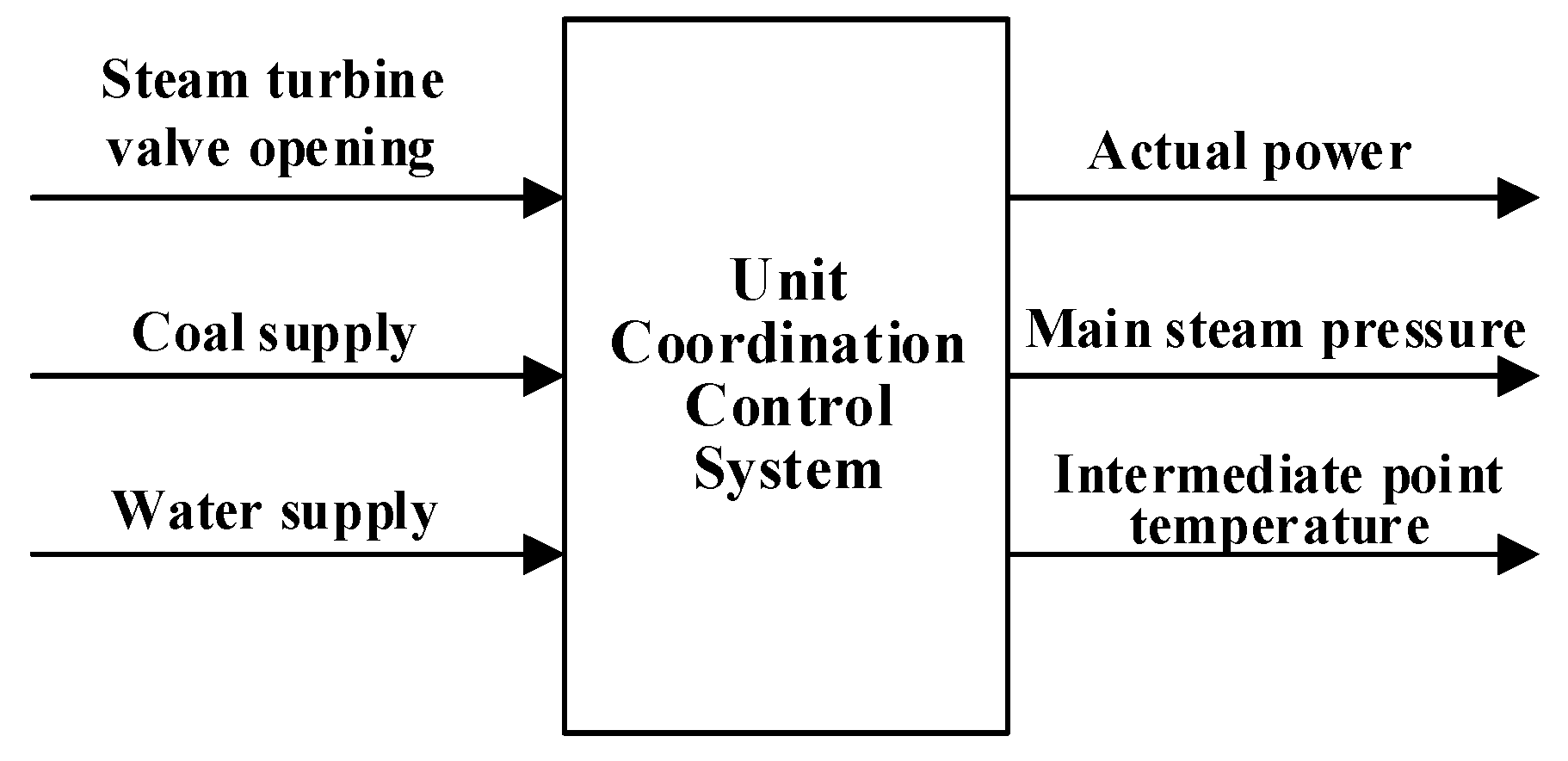
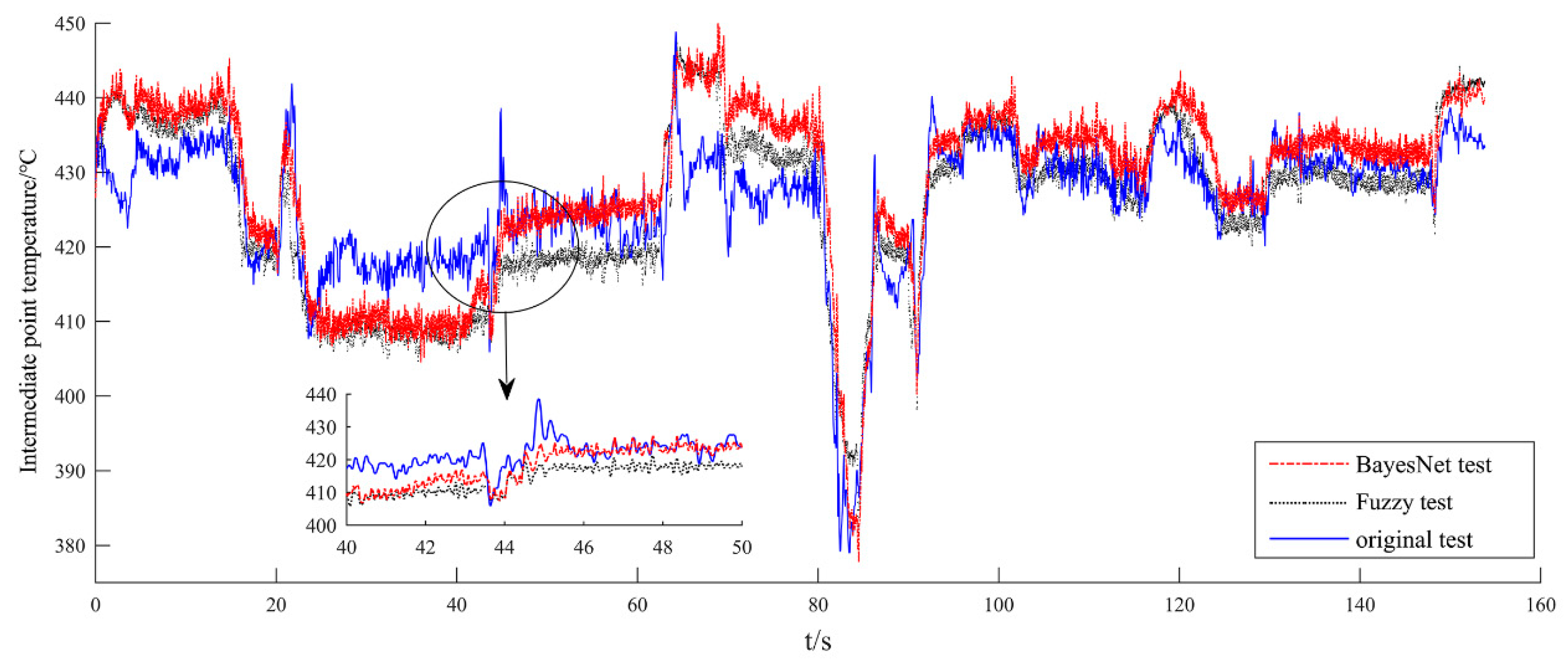
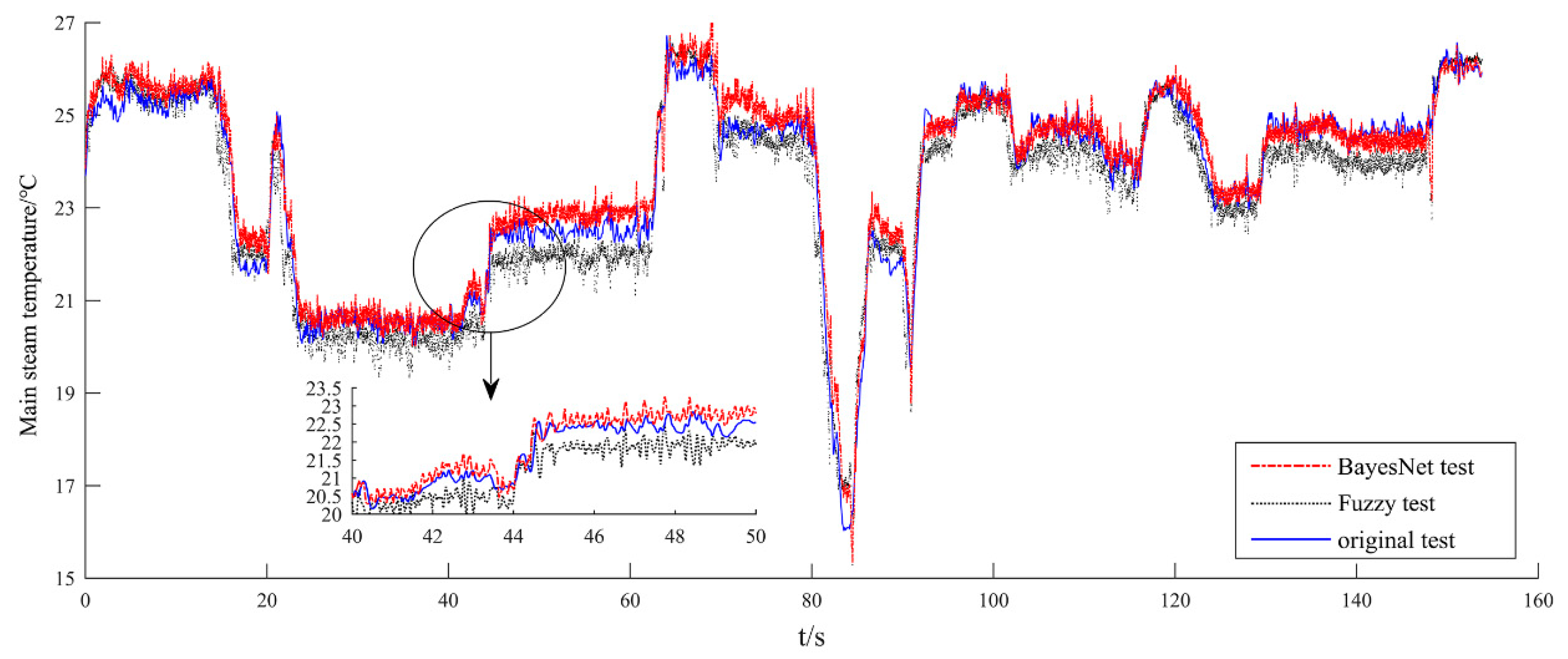
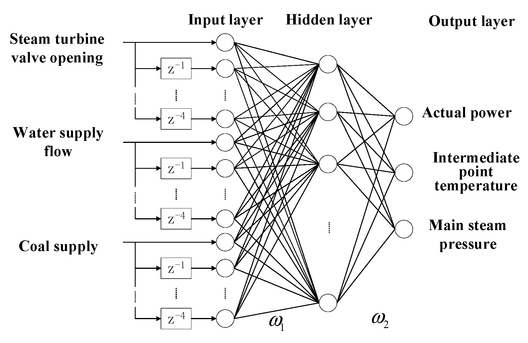
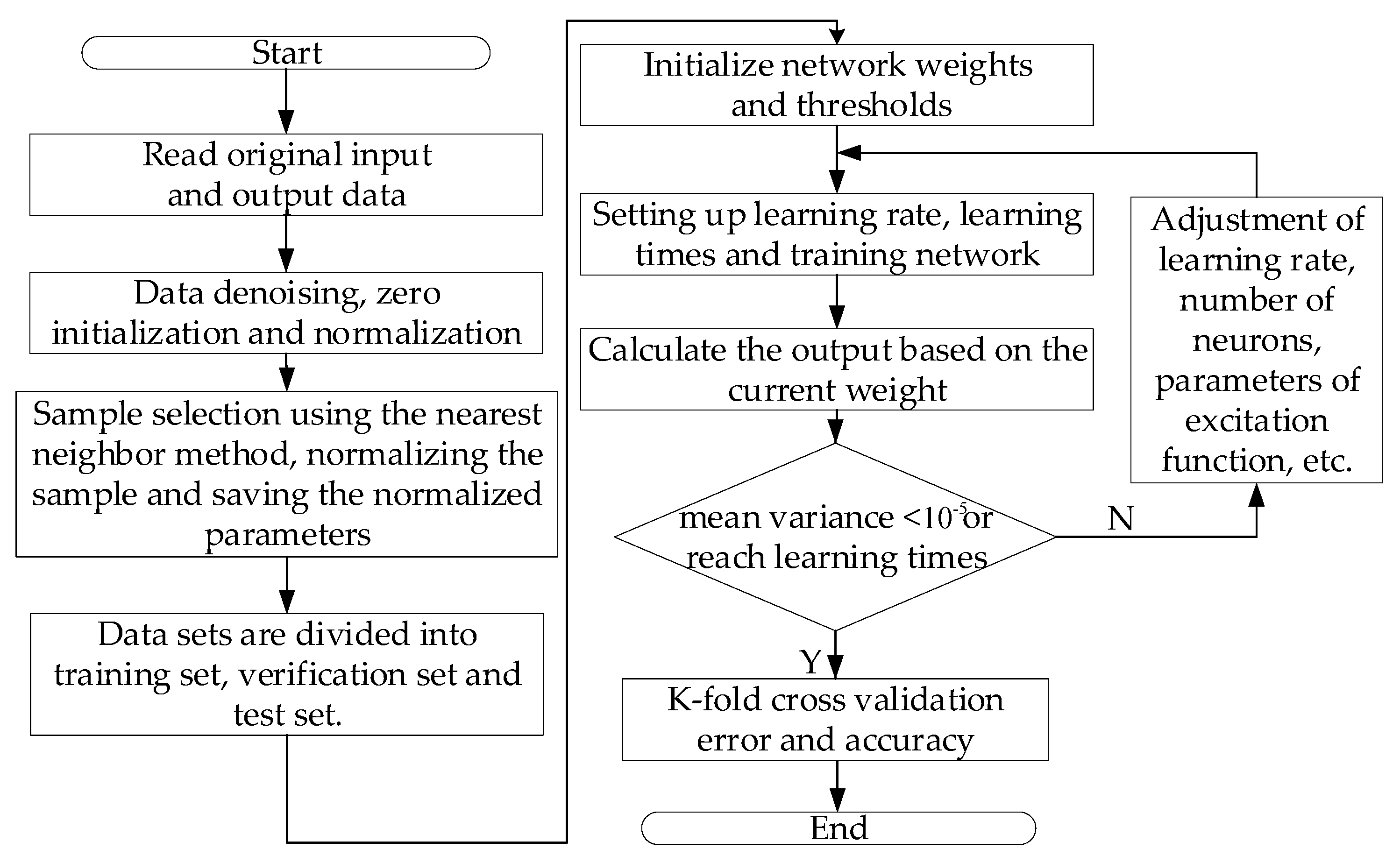
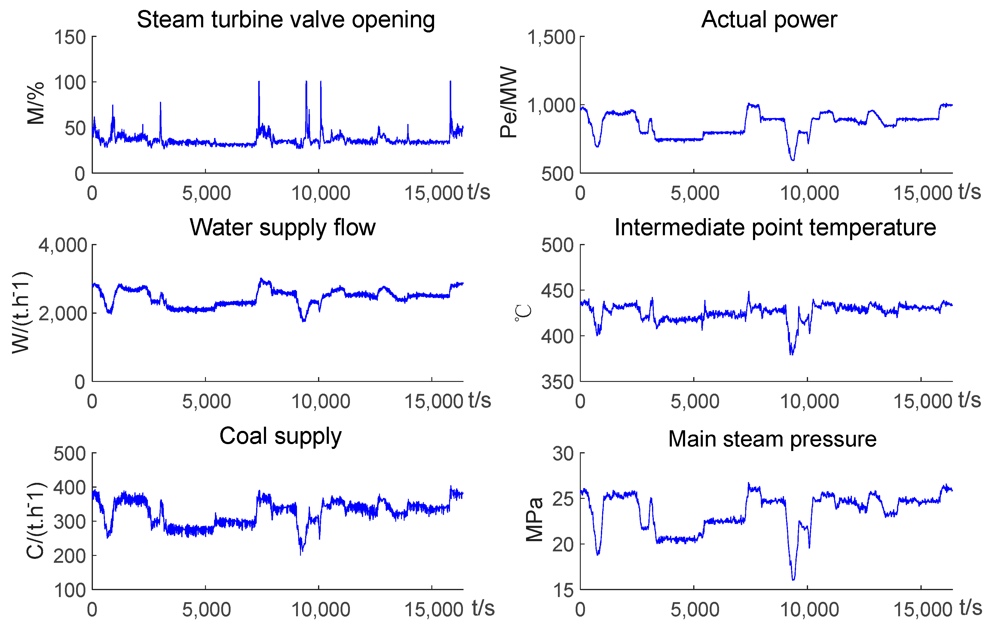
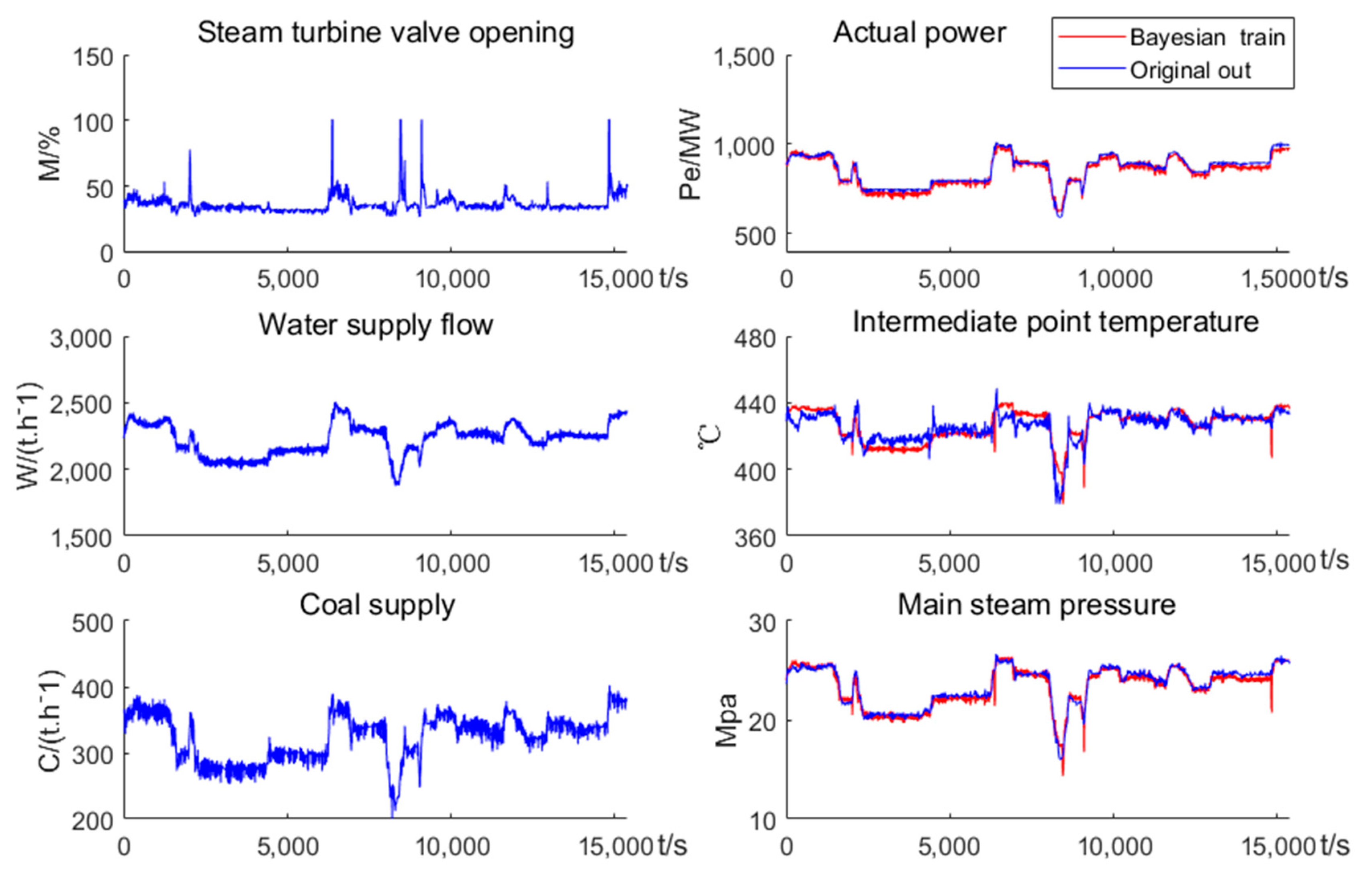
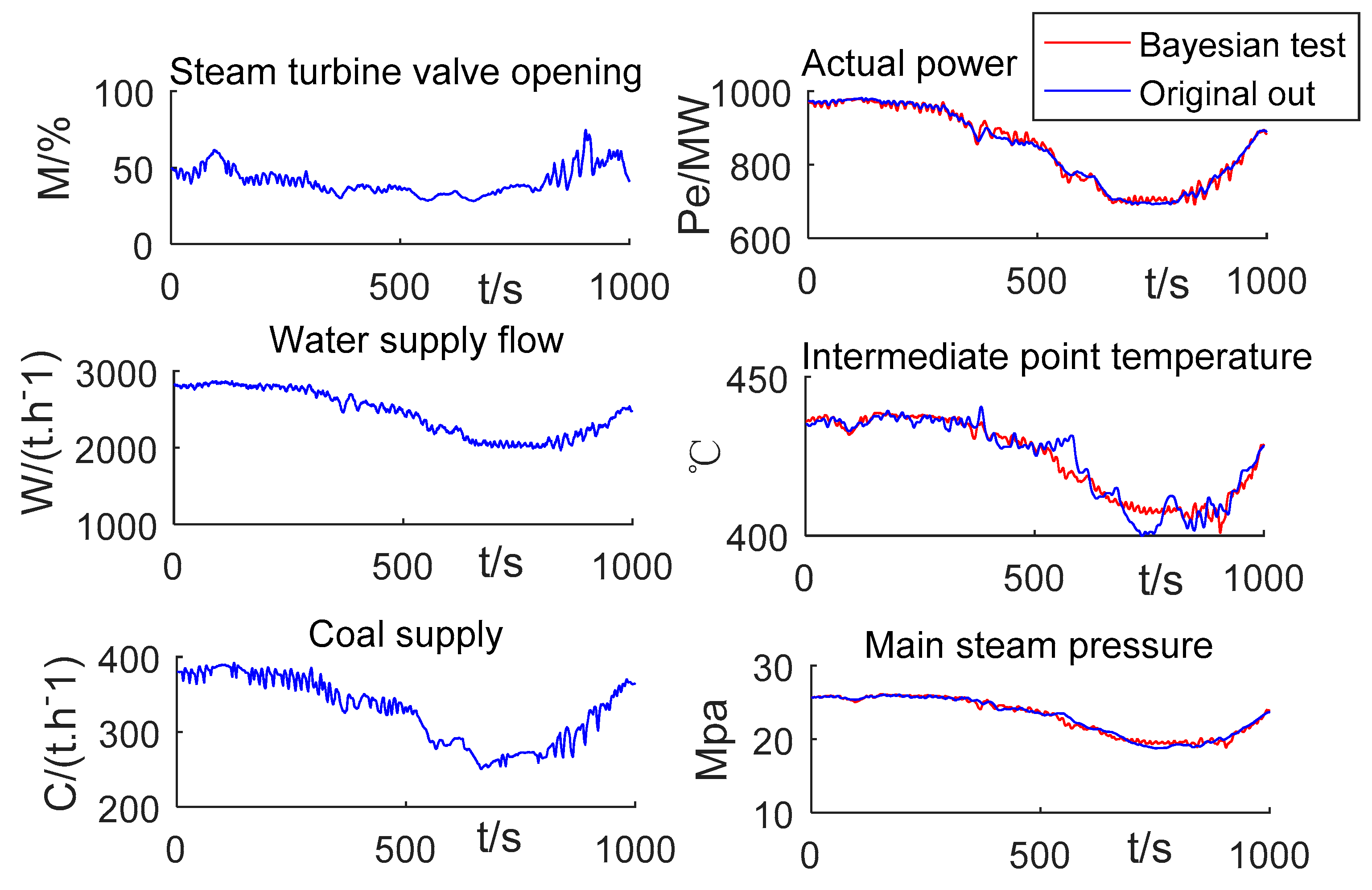
3.1. CCS Structure and Identification of AGC System

For the coordinated control system in AGC, the structure is also different for generating units with different capacities. For example, through a comparative analysis of subcritical units and supercritical units, subcritical units need to exist in the form of a steam–water mixture, so subcritical units require the use of a drum boiler. However, supercritical units operate using direct gasification, so they require the use of a once-through boiler. In system modeling, for the once-through boiler, the coal supply, water supply flow, and opening of the steam turbine valve will affect the length of each heated section in the steam water process, resulting in changes to parameters such as the actual power, superheated steam temperature, and main steam pressure [37]. Because the response of the main steam temperature at the outlet of the boiler to the boiler instructions is delayed considerably, an intermediate temperature (outlet temperature of the steam–water separator) is generally regarded as the regulated quantity. Therefore, the coordinated control system of the once-through boiler unit has the characteristics of strong non-linearity and strong coupling. It is a three-input/three-output multi-variable system. Specifically, there are the inputs of coal supply, water supply flow, and opening of the steam turbine valve opening, and the outputs are the unit’s actual power, intermediate temperature, and main steam pressure. The model of the CCS is shown in Figure 4.
The three inputs of CCS are water supply flow W , coal supply C , and steam turbine valve opening μ T . The temperature of the intermediate point T , main steam pressure P T , and actual power N e are the three outputs of the control system, as shown in Figure 4. The general transfer function model is more complex because of the strong coupling of the coordination system. Specifically, it needs to be expressed by nine polynomials; moreover, the model error is large. In this paper, in order to reduce the complexity of the mathematical model, a Bayesian neural network was used to identify a black-box model for the coordination system. The topological structure of the Bayesian neural network is shown in Figure 5.
The structure of the Bayesian neural network model includes the input layer, the hidden layer, and the output layer. The basic unit of the neural network is a neuron, and weights connect the neurons in each segment. Network topology, system samples, and training algorithms can affect neural network learning and adaptability. As for how to set the number of neurons, there is no excellent theoretical support at present, and it only relies on empirical values. After many tests, this paper chose the classical three-layer neural network model.
The two basic concepts of Bayesian theorem are prior distribution and posterior distribution. The key to the Bayesian inference method is that any inference must be based on a posterior distribution rather than on a sample distribution. When event A and event B are independent of each other, the greater the probability of B being observed, that is, the greater the prior probability of B, then the smaller the positive effect of B on the probability of occurrence of A is [29]. The Bayesian theorem is re-expressed as follows:
π ( x | θ ) = p ( x | θ ) π ( θ ) p ( x | θ ) π ( θ ) d θ .
In Formula (6), θ is an estimating parameter; x is sample information; π ( θ ) is the prior distribution density function of θ ; π ( θ | x ) is the posterior distribution density function of θ , which is an adjustment of the occurrence probability after new samples appear; p ( x ) and p ( x | θ ) are density functions of x , where p ( x ) is a normalization factor as follows [29]:
p ( x ) = p ( x | θ ) π ( θ ) d θ
It can be expressed as:
Prior distribution π ( θ ) + sample information x →posterior distribution π ( θ | x ) The ultimate goal of neural network training is to find the right weight vector ω in order to get the minimum root mean square error E. According to the Bayesian principle, the posterior probability of the weight vector is as shown in Formula (8) [29]:
P ( ω | D ) = P ( D | ω ) P ( ω ) P ( D ) .
In Formula (8), P ( ω ) is a prior probability distribution of weight vector ω , P ( D | ω ) is a likelihood function, and P ( D ) is the distribution of samples and is constant and independent of ω . Suppose that the prior distribution of ω is an exponential distribution as shown in Formula (9):
P ( ω ) = 1 Z ω ( α ) e 1 2 α ω 2
Assuming that the target value is y, the likelihood function is as follows:
P ( D | ω ) = i = 1 N P ( y | u , ω ) = 1 Z D ( β ) e β E D ( ω )
where, Z D ( β ) is a normalization factor, and β is a superparametric. As can be seen from Formulas (9) and (10), the posterior probability distribution is:
P ( ω | D ) = 1 Z S ( α , β ) e S ( ω ) .
where, S ( ω ) represents the regular error function, and Z s ( α , β ) is a normalization factor, so:
Z S ( α , β ) = e S ( ω ) d ω .
If the weight matrix ω causes the posterior distribution probability P ( ω | D ) to take the maximum value, then S ( ω ) takes the minimum value at this point. Thus, the weight optimization problem is transformed into the solution of the minimum problem.
The data at the current moment and the first five moments are taken as neuronal input to establish the relationship in state space and consider the influence at a certain time. There are 15 neurons in the input layer, and the input U of neurons can be expressed as:
U = [ u ( k ) u ( k 1 ) u ( k N + 1 ) ] N × 1 .
Among them,
u ( k ) = [ u 1 ( k ) u 2 ( k ) ] N × 1 .
The number of neurons in the hidden layer cannot be calculated according to the theory. According to the results of many experiments, it is set to 23. The weight matrix from the input layer to the first hidden layer is ω 1 , and the activation functions are hyperbolic tangent functions.
f 1 ( x ) = 1 e 2 x 1 + e 2 x .
The weight matrix from the hidden layer to the output layer is ω 2 , and the positive proportion function is chosen as the excitation function. Bayesian neural network modeling is shown in Figure 6. The optimization procedure of Bayesian neural network modeling algorithm is shown in Table 1.
f 2 ( x ) = x .
Based on the historical operation data of a 1000 MW ultra-supercritical unit, opening of the steam turbine valve, the water supply flow, and coal supply were collected as the inputs of the model, and the actual power, intermediate point temperature, and main steam pressure were taken as the outputs of the model. A total of 16,381 sets of data were collected with a sampling interval of 0.01 s. The input and output curves are shown in Figure 7. All data shown in the figure are unprocessed, original data.
After preprocessing all data, such as zero initialization, denoising, normalization, and so on, the nearest neighbor method was used to select 15,000 sets of data for the sample data, and the rest of the data were used as test data using the Bayesian neural network algorithm. The training results are shown in Figure 8.
It can be clearly observed that the training errors of the actual power and main steam pressure by the Bayesian neural network methods were small, while the training error of the intermediate point temperature was larger, especially during rapid decline or rise. The reason for this problem is that the output of CCS has a strong coupling relationship. When the actual power and main steam pressures are functioning at their best, the intermediate point temperature will be slightly inferior to ensure that all the output results remain at their best. After model training was completed, the rest of the data were subjected to a verification test, and the test results are shown in Figure 9.
The training error of the Bayesian neural network decreased rapidly from 2780 to 153 in the first 1000 generations and then changed slowly to an optimal value until the end of training. The final error was 7.4576. The training results indicated that the Bayesian neural network had weak advantages in the testing stage. However, the model error was still small, and the convergence speed of the Bayesian neural network was fast.
The performance of the model needed to be evaluated using corresponding performance indices. This paper used the K-fold cross-validation method, which is usually used in engineering to verify the error and accuracy of the model, in order to evaluate the identification model trained by the Bayesian neural network. The model never used any information related to the test set during the K-fold cross-validation analysis, so the performance of the final model in the test set was more reflective of its true performance. At the same time, over-fitting problems of the model could be improved because the test model ultimately selected the model with the best performance in the verification set rather than the training set. The K-fold cross-validation procedures are as follows:
Step 1:
The original data were randomly divided into K parts, and this paper used K = 4;
Step 2:
One part was selected as the validation set, and the remaining K-1 was selected as the training set to train the model. After training, a model was obtained, and the model was verified with its corresponding verification set while, at the same time, recording the error and accuracy of K-fold cross-validation;
Step 3:
Step 2 was repeated K times, and the average of error and accuracy of K-fold cross-validation were calculated. This ensured that each subset had the opportunity to serve as a verification set and a training set so that the training and verification samples were distributed uniformly;
Step 4:
Test sets were used to test the trained identification model and record the error and accuracy of K-fold cross-validation.
According to the above steps, the error and accuracy of K-fold cross-validation and its mean value obtained by K-fold training are shown in Table 2.
The results of using the test sets to test the identification model were a K-fold cross-validation error of 2.0053 and an accuracy of 92%. According to the above cross-validation results, the Bayesian neural network identification method studied in this paper can be applied to the CCS.
In order to further prove the reliability of the Bayesian neural network model, this paper compared it with the fuzzy model proposed by Wu X et al. [25]. The concrete results are shown in Figure 10, Figure 11, Figure 12 and Figure 13.
From comparisons of the test charts, it can be seen that the test results of the two methods were obviously different. The fluctuations of the actual power and the main steam pressure curves were significantly smaller than that of the intermediate point temperature curve. Although the trend of fuzzy identification was basically correct, the accuracy was not as good as the Bayesian neural network. In combining the identification results of the three outputs, the Bayesian neural network was advantageous in the testing stage because its model error was still small and the convergence speed of Bayesian neural network was fast. Therefore, the identification results of the Bayesian neural network are reliable and can be applied to subsequent research.

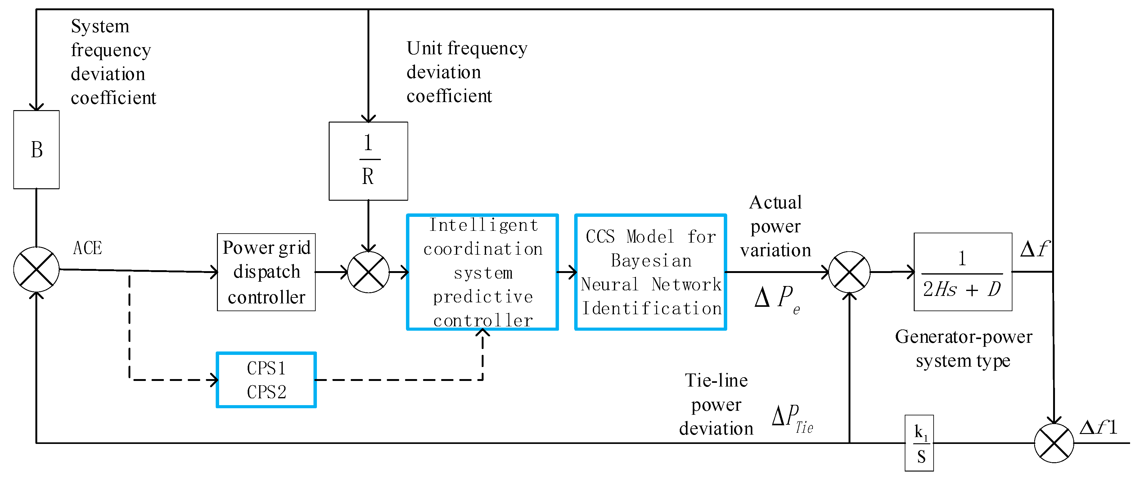
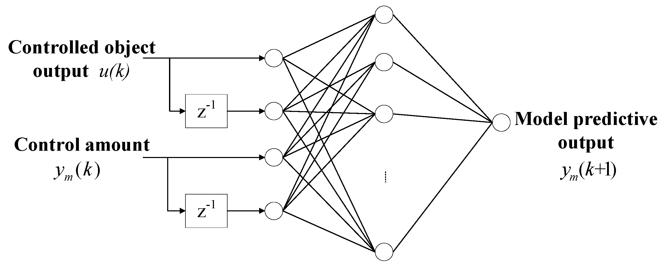
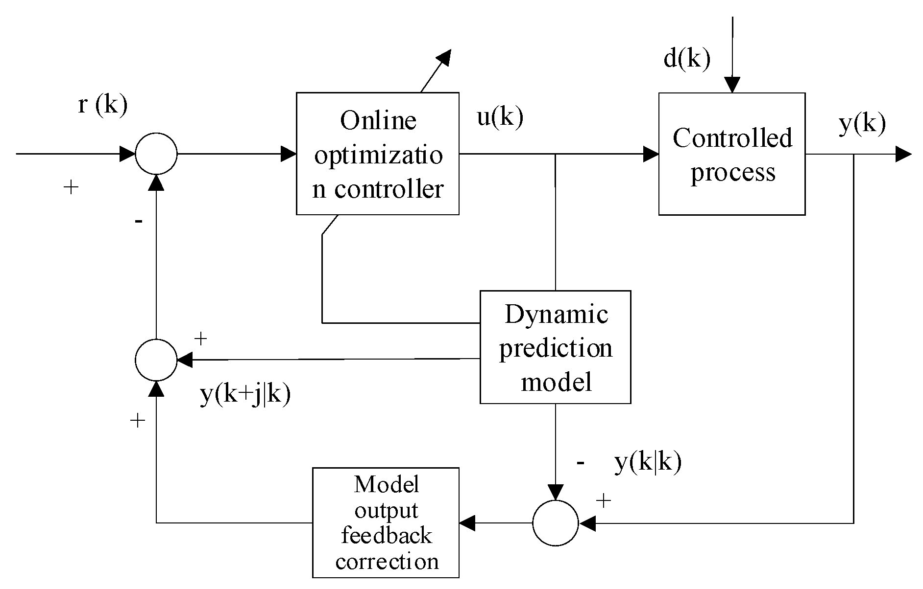
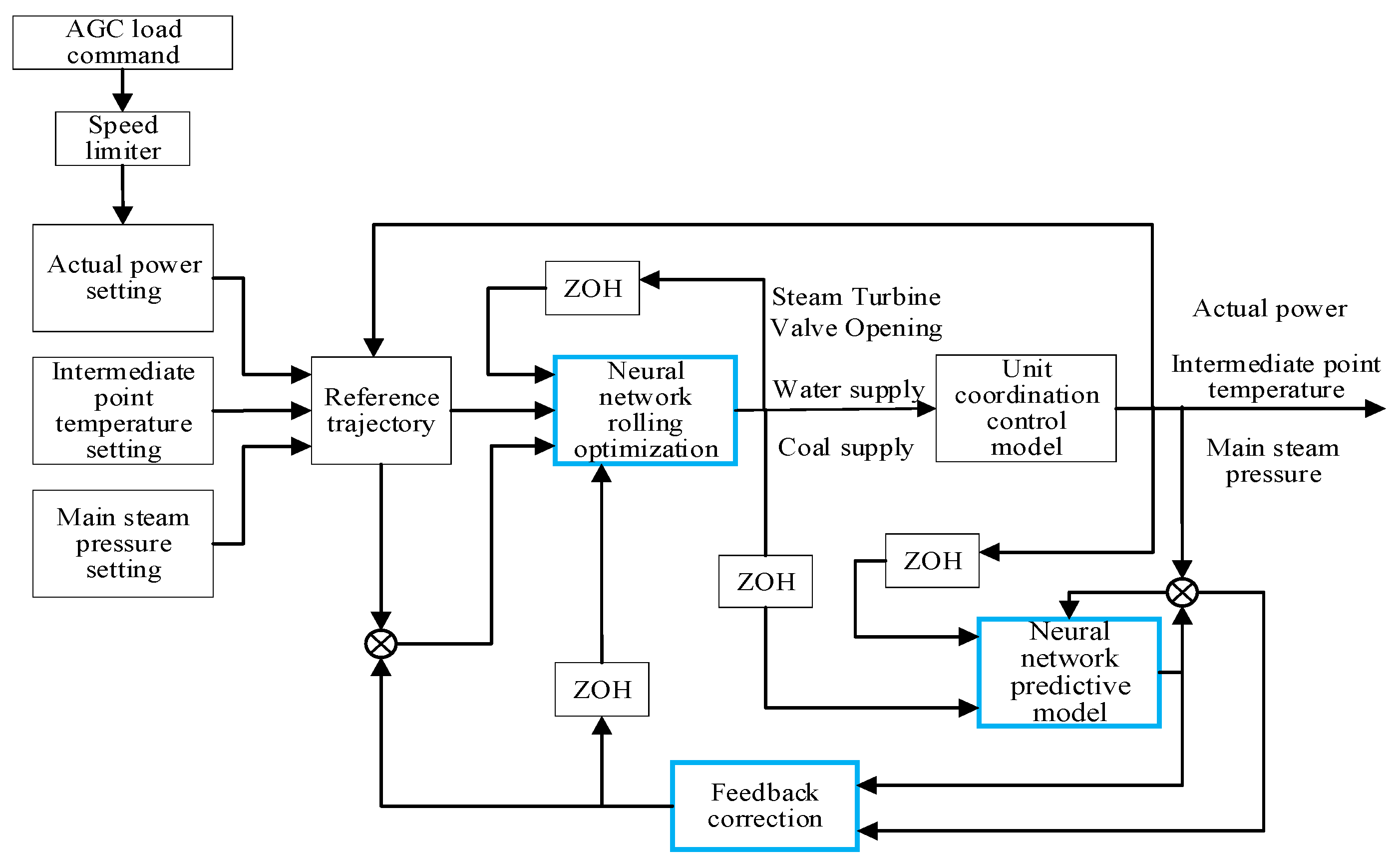
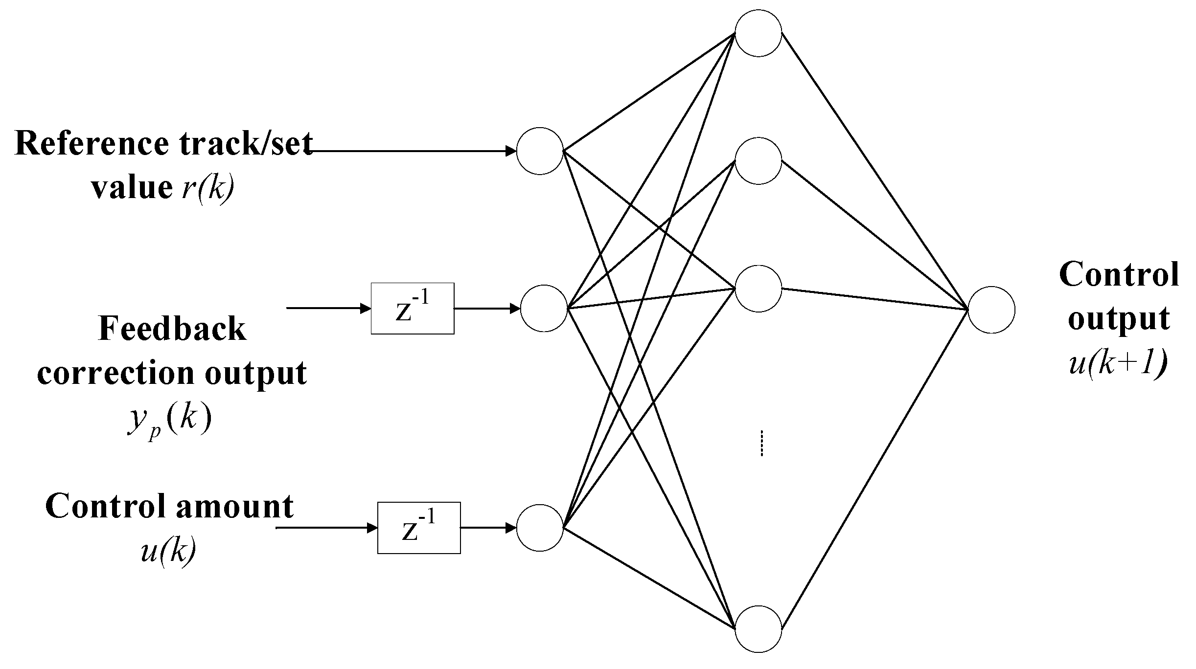
3.2. Design of an AGC Intelligent Predictive Control System Based on CPS.

Predictive control is a new type of control algorithm that include multi-step testing, rolling optimization, and feedback correction. It is especially suitable for controlling those industrial production processes for which it is difficult to establish accurate mathematical models. The classical predictive control structure is shown in Figure 13.
The prediction model refers to the dynamic model of the system, which can predict future time outputs with knowledge of future time inputs. Rolling optimization refers to finding the optimal control sequences that can optimize the objective function with the current state of the system and the prediction model in each sampling period, and the first element of the optimal control sequence is implemented in the controlled process. Feedback correction is primarily used to compensate for the prediction error and model mismatch.
The CCS model of the AGC system established in this paper is a black-box model trained by the neural network. Then, the structure of the AGC intelligent predictive controller was designed by combining artificial intelligence and classical predictive control ideas, as shown in Figure 14. Similar to the general predictive control structure in Figure 13, a neural network predictive model, feedback correction, and rolling optimization by neural network methods constituted the new AGC intelligent predictive control system. In Figure 13, ZOH refers to the zero-order keeper, which functioned by keeping the current sampling data until the next moment.
(1) Neural Network Predictive Model
As the primary element in predictive control, the task of the prediction model is based on the inputs of CCS at the current k-time, the next (k + 1) moment, and the output of the system at the k-time, which predicts the k + 1 output. In this paper, an accurate CCS simulation model was obtained through Bayesian network identification, as the effect of the prediction model was completely consistent with the effect of the Bayesian network model in CCS identification. Therefore, the mean square deviation of the known Bayesian neural network model was taken as the objective function of the model prediction network. The topological structure of the model prediction neural network is shown in Figure 15.
Then, in the topological structure of the model prediction neural network, the current time control quantity u(k), the future time control quantity u(k + 1), and the current time output quantity y m ( k ) are the inputs of the prediction model. The output prediction value y m ( k + 1 ) of the k + 1 time is the output of the prediction model. In addition, the mean square errors of the prediction output and the output of the CCS identification models are chosen as the objective functions.
(2) Feedback Correction
In the actual operation of power plants, there are always uncontrollable disturbances or unexpected situations, which lead to errors in model prediction. Feedback correction is achieved by collecting the output y ( k ) of the actual object. Deviation e m ( k ) is used to correct the predicted output y m ( k ) of the existing predictive model [38], and the output value of the predictive model can be adjusted in real-time according to the actual process.
e m ( k ) = y ( k ) y m ( k ) .
After feedback correction, the output of the prediction model is revised from y m ( k + 1 ) to y p ( k + 1 ) [38]. In Formula (11), h is the error correction coefficient [39], whose value is adjusted according to the actual operation of the specific system.
y p ( k + 1 ) = y m ( k + 1 ) + h × e m ( k ) .
(3) Neural Network Rolling Optimization
The core idea of predictive control is to decompose a long-term optimal control problem into several short-term optimization problems. By selecting the predictive horizon, rolling optimization achieves the optimal control sequences in each short-term period. The fundamental difference between intelligent predictive control and classical predictive control lies in the design of the rolling optimization module. This paper chose the neural network algorithm for rolling optimization, and its topology is shown in Figure 16.
The inputs of the rolling optimization module are the current time control value u ( k ) , the current time output value y p ( k ) , and the current time setpoint value r ( k ) . The objective function, as shown in Formula (19) [40], minimizes the sum of squares of errors between the setpoint values r ( k + i ) and the output values y p ( k + d ) of the predictive model. By on-line learning, the next control value u(k + 1) can be predicted.
min J = [ r ( k + d ) y p ( k + d ) ] 2 2 .
In the actual operation of power plants, in order to ensure the safety and efficiency of equipment, step jump reference signals are generally not allowed. Thus, the general expression of the reference trajectory after smoothing is as follows:
y r ( k + 1 ) = α r y ( k ) + ( 1 α r ) × r ( k )
In the AGC system, the above intelligent predictive control strategy was used as the control mode of CCS. However, the traditional PI control mode was still used in the power grid dispatching controller. The complete AGC feedback control system was composed of a traditional PI control mode, a generator power system model, and a regional deviation coefficient. The specific steps of the intelligent predictive control algorithm were shown in Table 3.

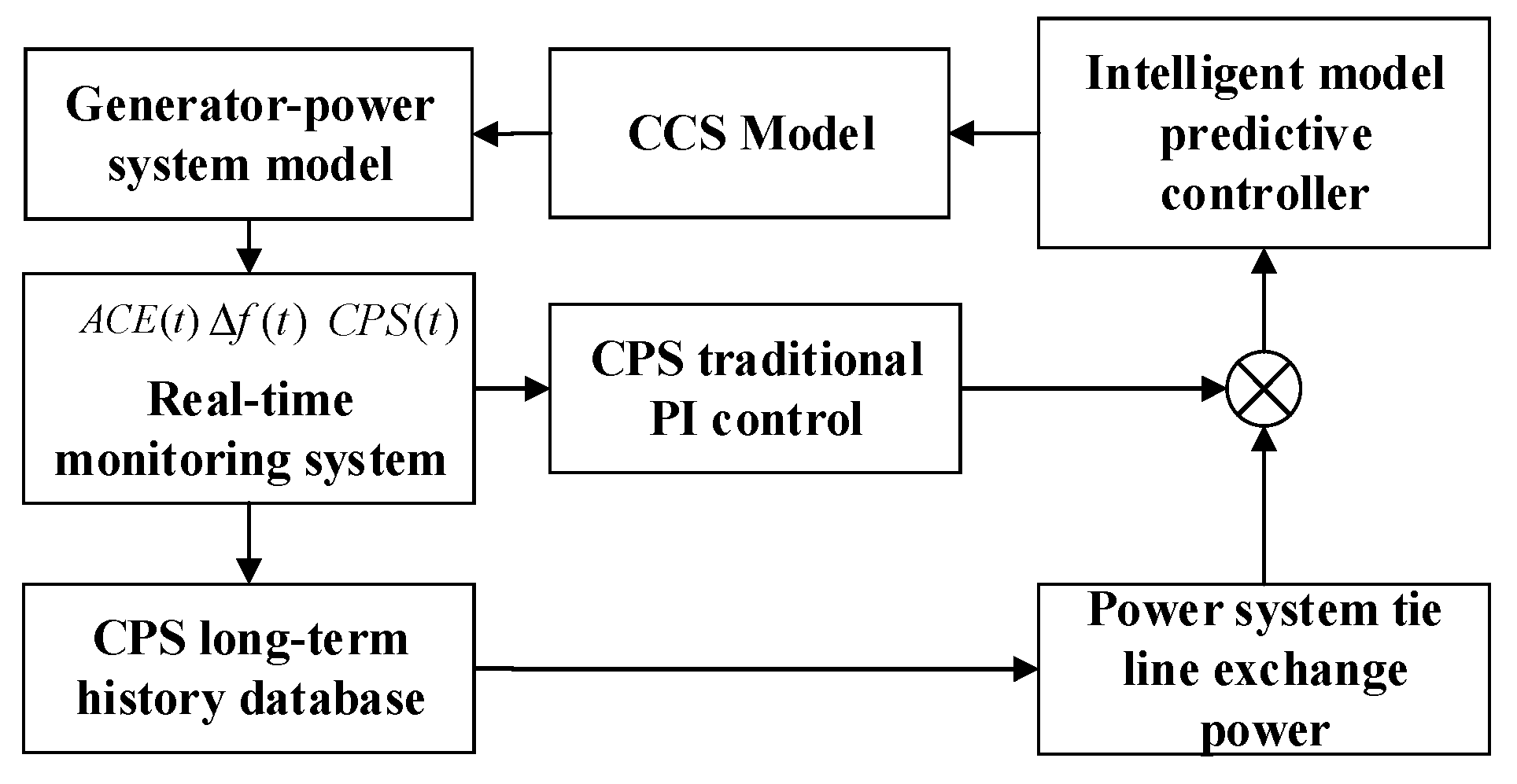
3.3. CPS Control Principle in a Multi-Area, Interconnected Power Grid

The actual operating power system is a large-scale system mainly composed of multiple regional power grids, and mutual power support is provided between different areas through tie lines. If multiple units are interconnected, tie lines and frequency bias control (TBC) are used to form the TBC–TBC mode of the interconnected grid for ACE.
In the TBC–TBC mode, frequency fluctuations are small when the parameters are selected reasonably. No matter where the load disturbance occurs, there will be no control actions in other areas except the in the disturbance area. In effect, balancing the real-time load disturbance can be realized. In a modern interconnected power grid, if the capacity of the frequency modulation units in each area is sufficient, this control mode is generally adopted. When load disturbance occurs in the system, the active power of the units can be regulated by the AGC system. Finally, ACE caused by power exchanges and frequency deviations of tie lines can be stabilized to zero, and the following formula is calculated [31]:
A C E = Δ P t i e + B Δ f .
Therefore, the following can be obtained:
A C E × Δ f = Δ P t i e × Δ f + B Δ f 2 .
According to the requirements of CPS, it is hoped that CPS1 will be greater than 200% for as long as possible, or when meeting the requirements of CPS2, the relationship will be 100 C P S 1 200 % . Therefore, it is desirable for the value of CF to be a negative or positive value that is as small as possible. It can be known from Equation (22) that CF has a negative value, and Δ P t i e and Δ f can only have opposite signs, so Δ P t i e and Δ f have opposite physical meanings.
When the increased load leads to a lower frequency in the area, Δ f is negative. At this time, other areas are required to support power generation in the area. Δ P t i e is positive, and the power generated in the area is increased so that the frequency increases and returns to the set value.
When the decreased load leads to a higher frequency in the area, Δ f is positive. At this time, the area can support power in other areas. If Δ P t i e is negative, the power generated in the area is reduced so that the frequency is reduced and returns to the set value.
In summary, when Δ f and Δ P t i e are opposite, it is very beneficial to the stability of the grid frequency, and the CPS index evaluation criteria are confirmed. Conversely, when Δ f and Δ P t i e are the same, it indicates that the adjustment behavior of the region at this time will endanger the stability of the grid frequency, so Δ P t i e × Δ f must be made as small as possible. Δ f 2 reflects the requirement for frequency deviation, which is positive in itself, so it must be as small as possible.
According to the characteristics of traditional CPS PI controllers, the power system is predicted and controlled by a new system, including an intelligent model predictive controller, a CPS real-time monitoring system, and long-term historical data set, which lead to good robustness and adaptability. The control structure of a region in a multi-region, interconnected system is shown in Figure 17.
Figure 17 mainly consists of the following parts:
(a)
A C E ( t ) / Δ f ( t ) / C P S ( t ) in the real-time monitoring system monitor the instantaneous values of ACE and CPS.
(b)
CPS in the long-term historical database records CPS statistics per hour, day, and year.
(c)
The traditional CPS PI controller consists of CPS1 and CPS2 controllers with PI structures, and a coordination controller. This coordinates the output of each controller in accordance with the standard CPS.
(d)
The intelligent predictive controller module predicts the next output of the power prediction system according to traditional PI control of the CPS and power system tie lines.

4. Simulation Analysis of the AGC Intelligent Predictive Control System Based on CPS

4.1. Test and Simulation of the Response Capability of the AGC system

The model of the 1000 MW turbine of a power plant was N1000-26.25/600/600 (TC4F), the main steam pressure rating was 26.25 MPa, and the frequency was limited from 47.5 Hz to 51.5 Hz. In the simulation test, the steam turbine was set to work under the sliding pressure mode, and both the unit load response and adjustment capability of the AGC system were tested.
The change of power of the unit was realized by adjusting the magnitude of the main steam pressure when a steam turbine operated under sliding pressure. As a result, the main steam pressure change was synchronized with the change of power of the unit. In the simulation test of this paper, the AGC load demand for the thermal power unit started by increasing the rated load by 10%, from 750 MW to 850 MW, and it increased again by 5%, from 850 MW to 900 MW, after running for 100 min. Two hundred minutes later, the AGC load demand decreased by 40%, from 900 MW to 600 MW. The intermediate point temperature setpoint remained unchanged, and the turbine pressure setpoint changed with the load demand. Results are shown in Figure 18, which indicate that the actual unit power output could quickly follow the changes of the load demand. It also shows that, after receiving the load demand, the steam turbine reacted faster than the boiler, which was reflected in the fluctuation of the intermediate point temperature.
During the simulation test process, the load overshoot was less than 2 MW, the frequency error accuracy was less than 0.2% P e , the main steam pressure fluctuation was small, and the intermediate point temperature was also within the allowable range. The AGC load demand response time was fast, which was within 10 s, and the adjustment time was about 9.3 min, which met the adjustment requirements.
Through the above analysis, it can be seen that AGC intelligent predictive control could realize the online automatic adjustments of CCS parameters. In addition, AGC intelligent predictive control enabled the system to track the AGC load demand more quickly so that the control performance of the entire closed-loop AGC system could be improved.

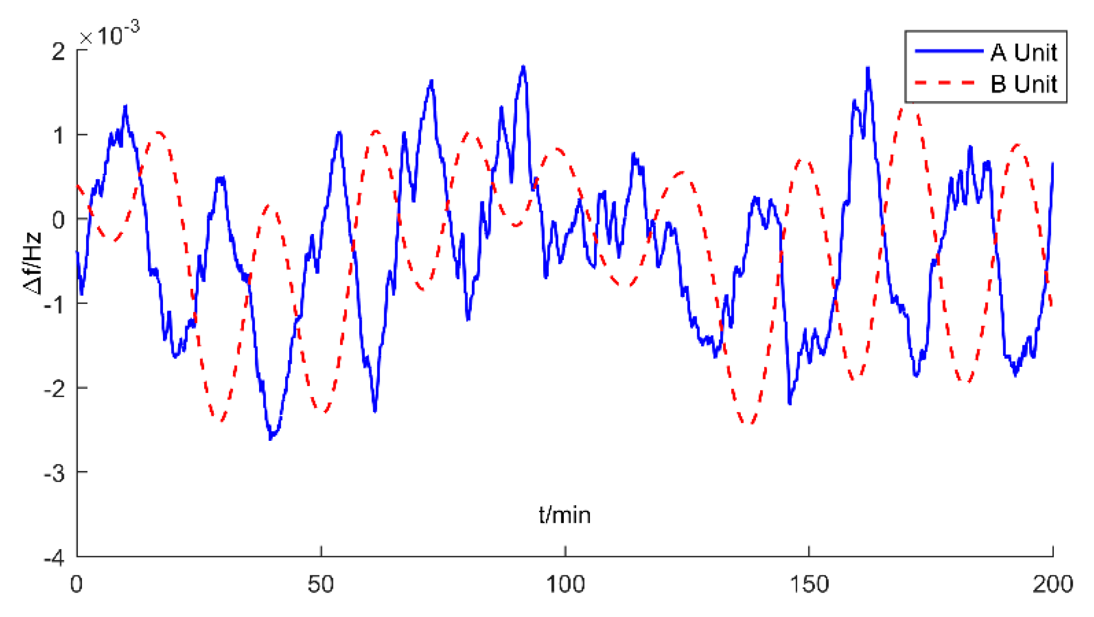
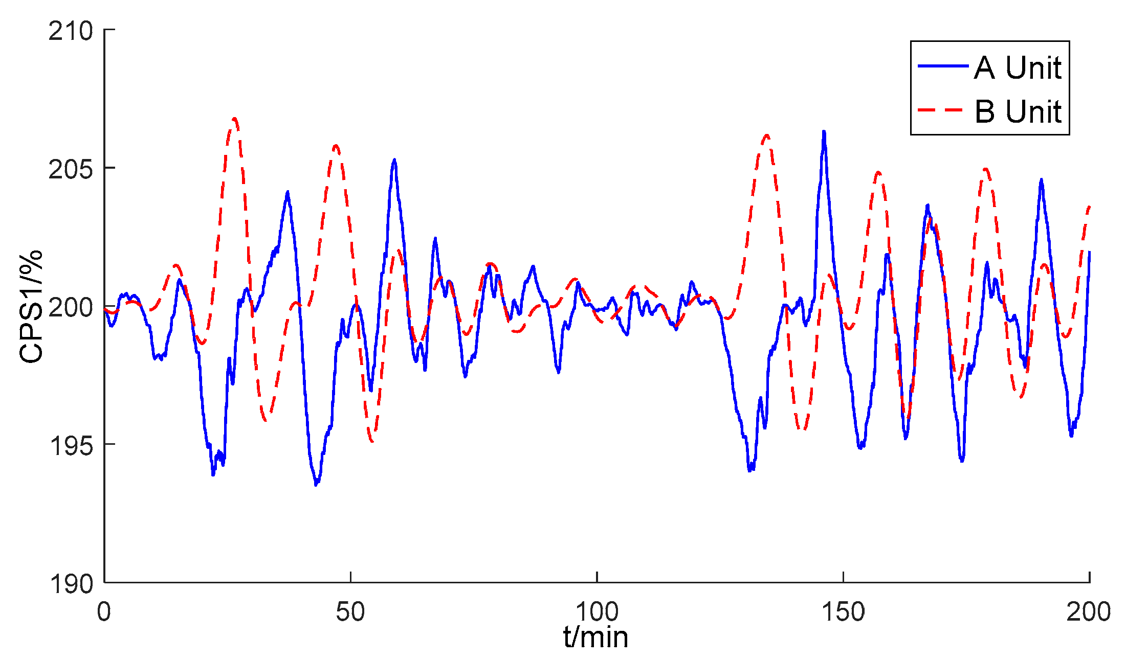
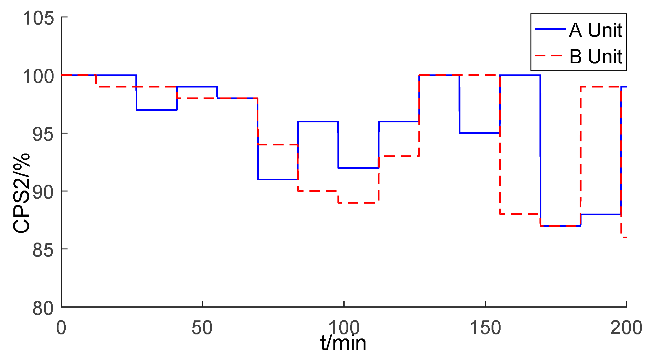
4.2. Analysis of the Control Effecst of Two Interconnected Units under CPS

According to NERC regulations, the performance of the regional AGC was evaluated according to CPS1 and CPS2 standards for the control area [33]. The control indexes should reach C P S 1 100 % and C P S 2 90 % . In connecting A and B units, area A and area B adopt tied line power frequency deviation control (TBC) to form the TBC–TBC mode of the interconnected power grid for ACE. In the simulation, as shown in Figure 19, there were two AGC units in the grid. White noise disturbance lasting 200 min was added to the generator side of unit A at Δ P f , and the overall range was approximately −20 MW to 20 MW. No disturbance was added to unit B, and no load change instructions were added to the two units.
At this time, the frequency deviation Δ f curves of the two units changed, as shown in Figure 20. When the disturbance was added, the frequency of unit B was significantly disturbed and changed rapidly. Under this change, unit B still compensated unit A and then changed with the frequency change of unit A. Under the total fluctuation range of 40 MW, the frequency changes of both units were in the normal range.
The variation curve of CPS1 under power disturbance to the generator side is shown in Figure 21. It can be clearly seen that after the unit A side was disturbed, the unit A CPS1 also had a corresponding change. When its CPS1 index value dropped below 200%, the CPS1 value of unit B rose randomly to about 206%. This showed that the ACE of unit B was beneficial to recover the frequency to the rated value at this time, and, to a certain extent, it could help unit A to maintain frequency stability of the entire regional network.
The variation curve of CPS2 under power disturbance to the generator side is shown in Figure 22. The average ACE was calculated once a minute in simulation, and the CPS2 standard was checked every 14 min. There were 14 checks in 200 min. The CPS2 of Unit A and unit B each had values two times less than 90%. Deviation between the simulation and the actual situation was considered, the threshold value was set differently in each grid, and sometimes the assessment adjusted them by 1.5 times. At the same time, all other indicators were within the required range, so the simulation results of the CPS2 standard were also within the normal range, indicating that the predictive control of the AGC model still had better control effects.
Tie lines are important links in regional interconnected power grids. It is also necessary to verify the impact of tie line disturbances on regional units. When units A and B were running stably and white noise was added to the tie line power, the disturbance range was about −10 MW to 10 MW. The variation curve of the simulation is shown in Figure 23. The range of variation was about −0.00148 Hz to 0.00138 Hz, which was within the allowable range of the system.
The CPS1 curve under tie line power disturbance is shown in Figure 24. The changes of CPS1 of the two units were consistent, and the range of variation was between 195% and 204.8%, which could meet the requirements of the index.
The CPS2 curve under tie line power disturbance is shown in Figure 25. The average value of ACE was calculated once a minute in simulation, and the CPS2 standard was checked every 14 min. Within 200 min, unit A had a value two times less than 90%, unit B had a value three times, and the overall index was above 85%, which basically met the requirements of power grid control.

5. Conclusions

Through the above theoretical derivation and simulation, the following conclusions can be drawn.
(1)
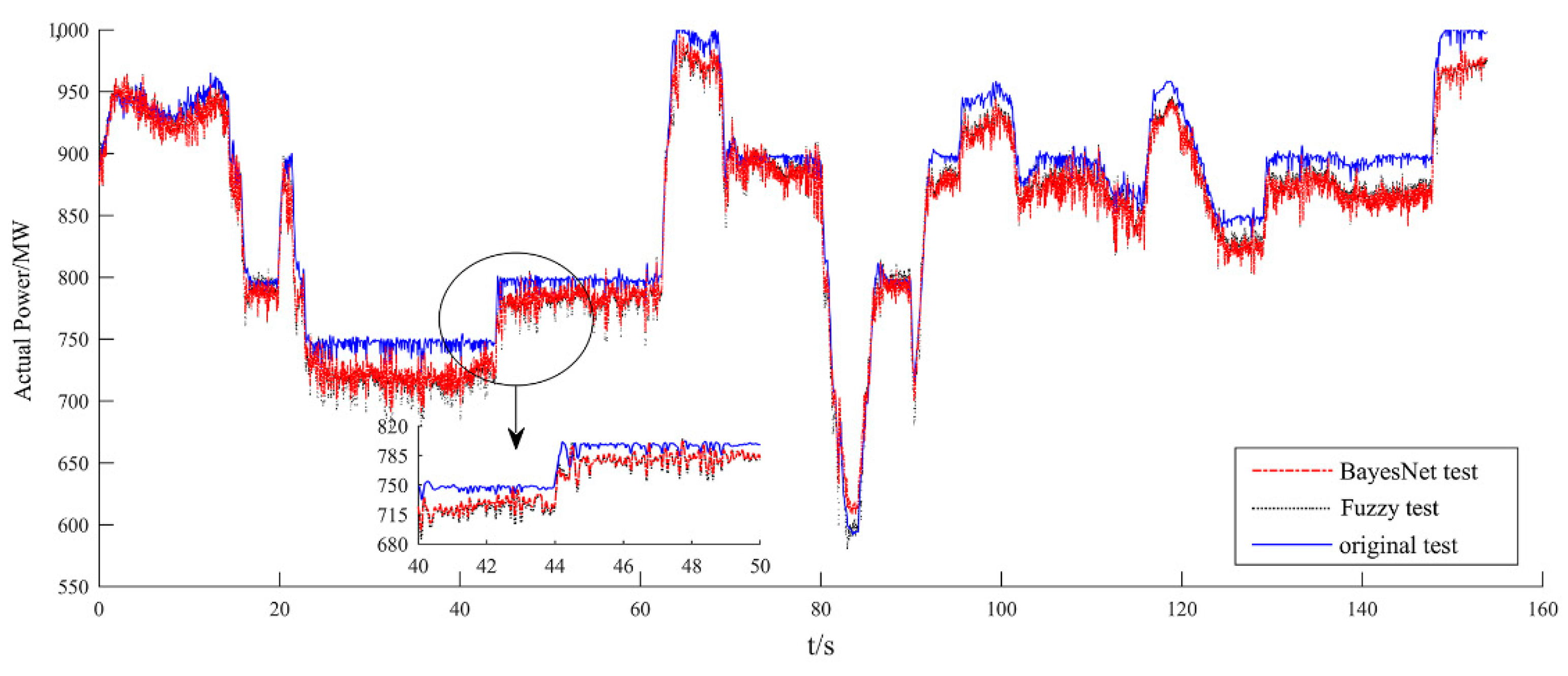
According to the field data, a CCS model was obtained through Bayesian neural network identification, which was regarded as the real model of the system. Through K-fold cross-validation and algorithm comparison experiments, the results showed that the Bayesian neural network had good recognition effect, and it was suitable for identifying CCS systems.
(2)
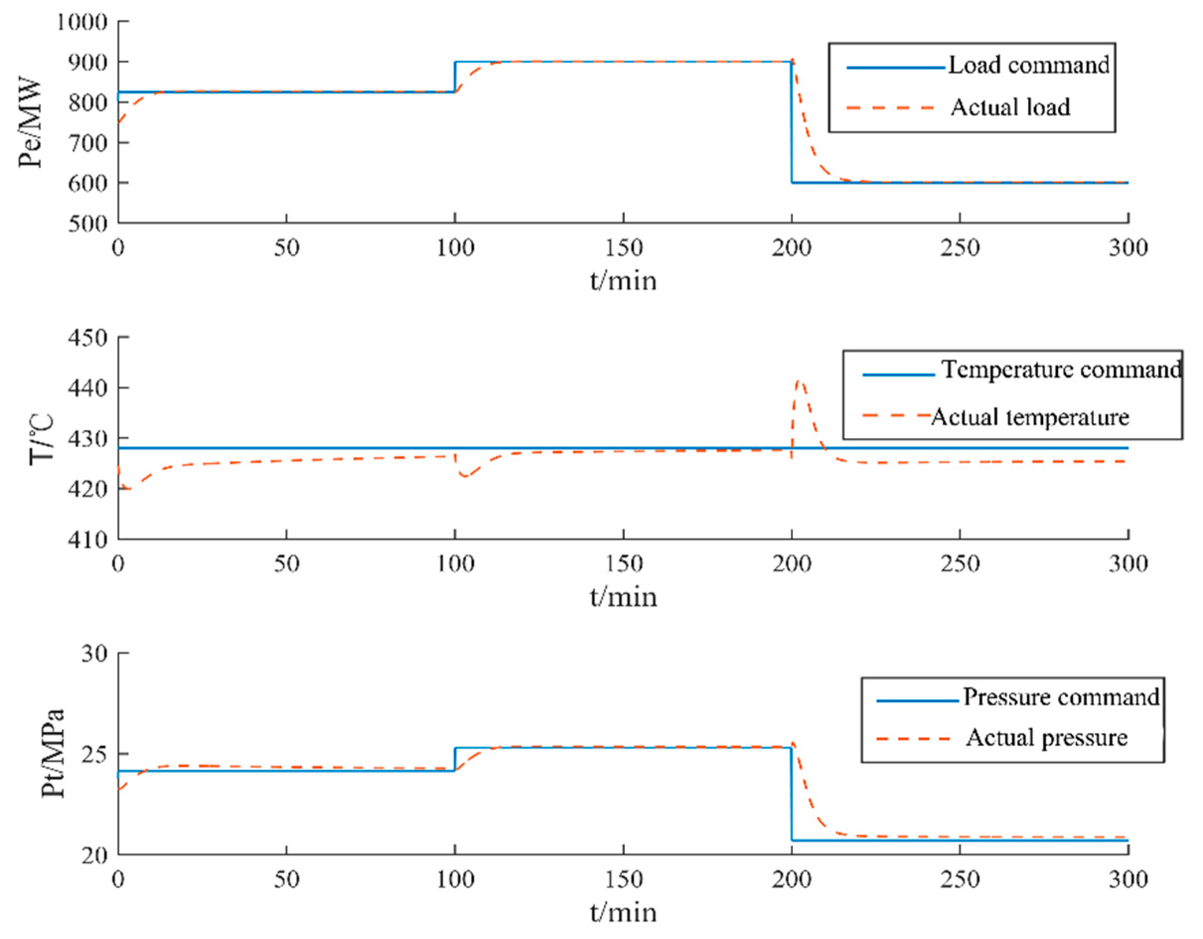
An AGC intelligent predictive controller based on CPS was designed and combined with predictive control and neural network ideas. It could improve the control performance of the system and achieved a good load, following effects under a sliding pressure operation mode.
(3)
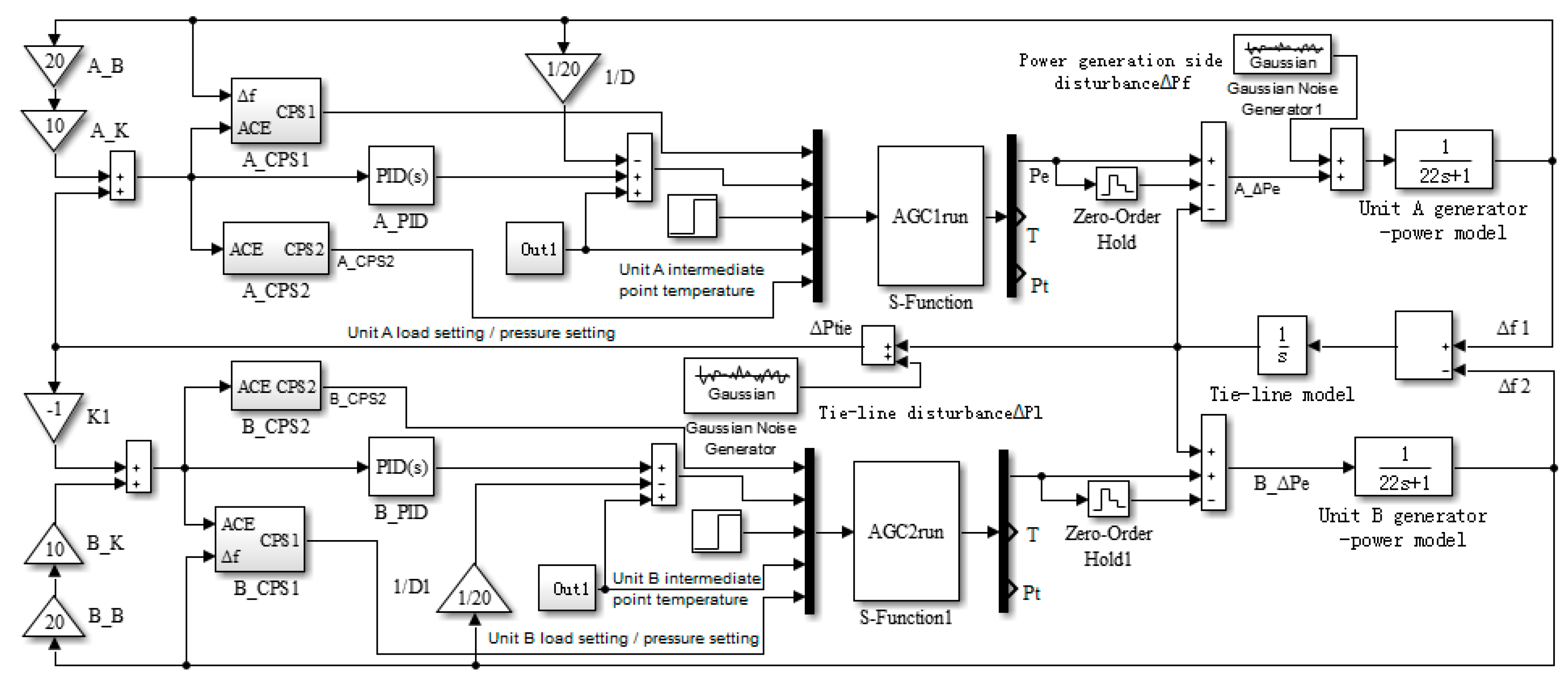
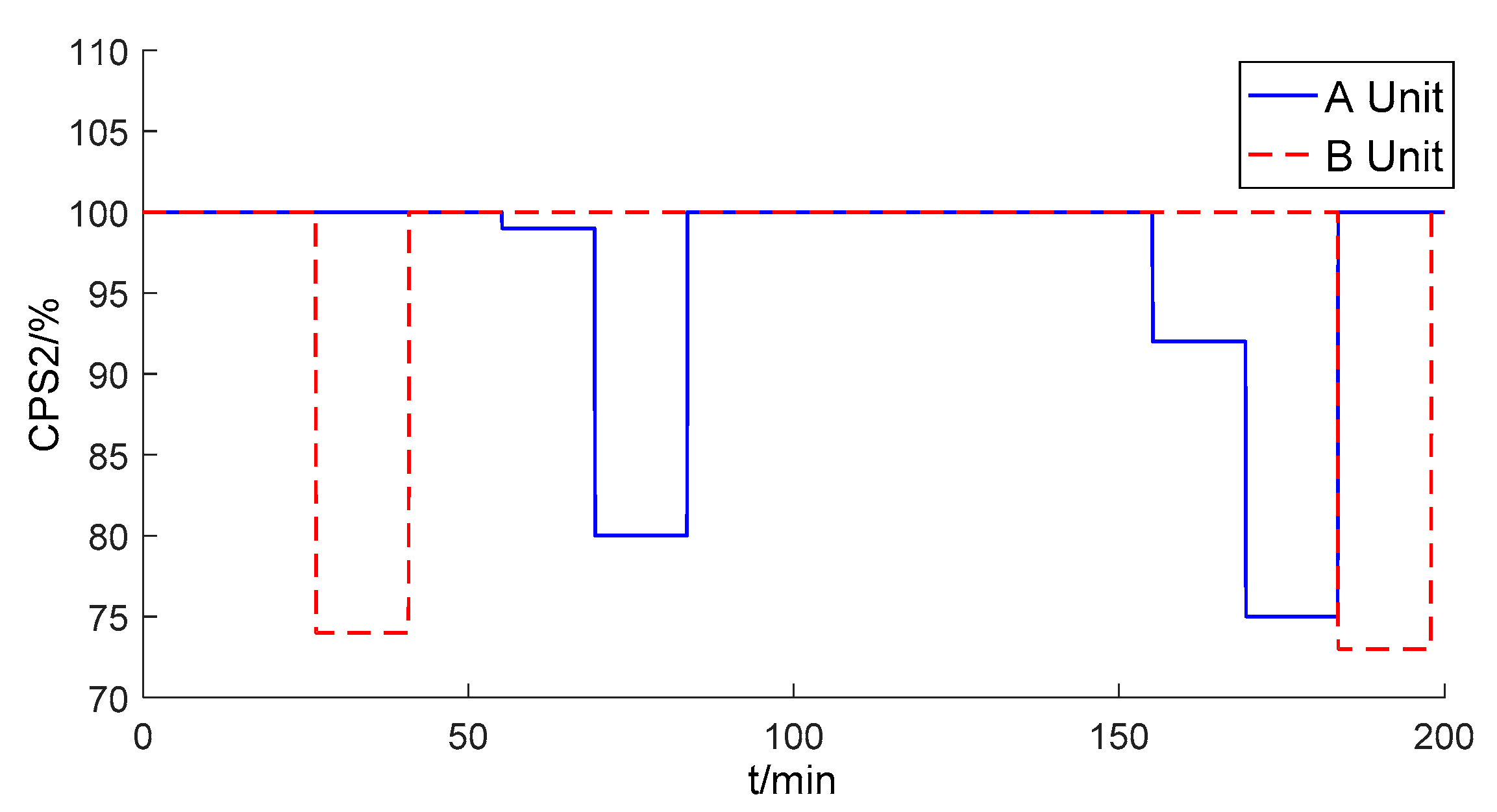
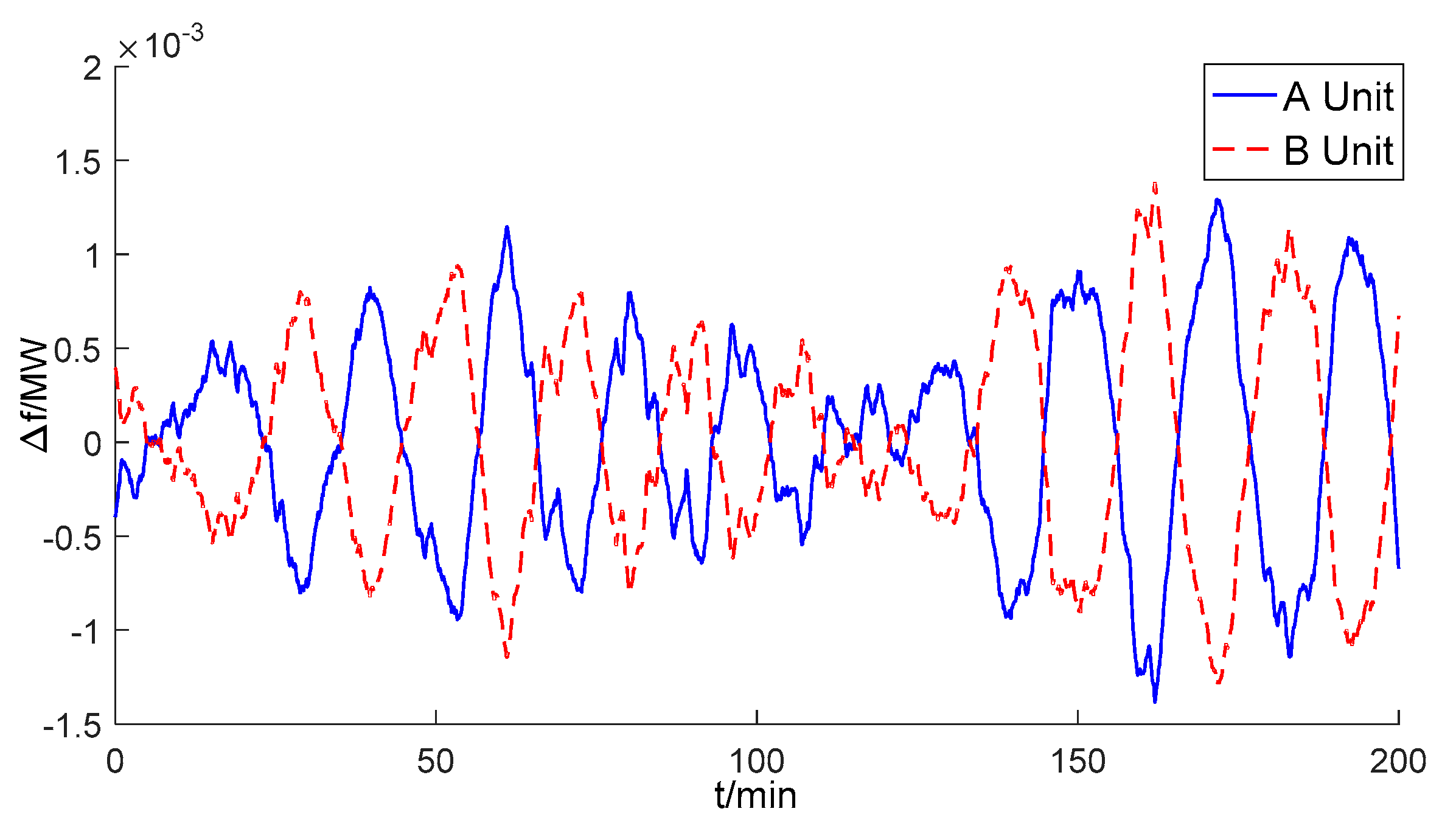
By introducing a CPS performance evaluation index that combined regional frequency and unit frequency deviations in detail, a two-unit interconnected simulation environment was established. The control effects of the AGC system under generator side and tie line power disturbances were simulated and analyzed. Results showed that the impact of AGC intelligent predictive control met the relevant regulations on load, frequency, and CPS index. It also pointed out that the evaluation of AGC control performance according to CPS1 and CPS2 standards was more suitable for the requirements of current power grid control.

Author Contributions

Conceptualization, D.P. and Y.X.; methodology, D.P. and Y.X. and H.Z.; software, Y.X.; validation, D.P. and Y.X. and H.Z.; resources, D.P.; writing—original draft preparation, Y.X.; writing—review and editing, Y.X. and H.Z.

Funding

This research was supported in part by Shanghai Science and Technology Commission Program (No.19511101600), in part by Engineering Research Center of Shanghai Science and Technology Commission Program (No.14DZ2251100).

Conflicts of Interest

The authors declare no conflicts of interest.

Nomenclature

H inertia coefficient of the generator ω weight vector
D per unit value of system load regulation P ( D | ω ) likelihood function
Δ P e actual power variation P ( D ) distribution of samples
Δ P T i e tie-line power deviation Z ω ( α ) normalization factor
Δ f frequency deviation α superparametric
f A actual frequency of the power grid Z D ( β ) normalization factor
f S planned frequency of the power grid β superparametric
P A actual switching frequency u ( k ) current time control value
P S planned exchange poweru(k + 1)the future time control value
B frequency deviation coefficients of the power grid y m ( k ) current time output value
C F coordination factorym(k + 1)prediction output value
B S total frequency deviation coefficient y ( k ) actual object output
L 10 ACE limit average in 10 min e m ( k ) feedback correction deviation
ε 1 m i n mean square root of mean frequency deviation in 1 min h error correction coefficient
ε 10 m i n mean square root of mean frequency deviation in 10 min y p ( k ) rolling neural network output
W water supply flow r ( k ) current time setpoint value
C coal supply flow
μ T steam turbine valve opening
T temperature of the intermediate pointAGCautomatic generation control
P T main steam pressureCPScontrol performance standard
N e actual powerEMSenergy management system
θ estimating parameterCCScoordinated control system
x sample informationTLBOteaching learning based optimization
π ( θ ) prior distribution density function of θ MPCmodel predictive control
π ( θ | x ) posterior distribution density function of θ NERCnorth American electric reliability council
p ( x ) density functions of x ACEarea control error
p ( x | θ ) density functions of x RTUremote terminal unit
ω 1 weight matrix from the input layer to the first hidden layerTBCtie-line and frequency bias control
ω 2 weight matrix from the hidden layer to the output layerDCSdistributed control system
P ( ω ) a prior probability distribution of weight vectorZOHzero-order holder

References

  1. Ismail, M.M.; Bendary, A.F. Load Frequency Control for Multi Area Smart Grid based on Advanced Control Techniques. Alex. Eng. J. 2018, 57, 4021–4032. [Google Scholar] [CrossRef]
  2. Hakimuddin, N.; Khosla, A.; Garg, J.K. Centralized and decentralized AGC schemes in 2-area interconnected power system considering multi source power plants in each area. J. King Saud Univ. Eng. Sci. 2018. [Google Scholar] [CrossRef]
  3. Kalavani, F.; Zamani-Gargari, M.; Mohammadi-Ivatloo, B.; Rasouli, M. A contemporary review of the applications of nature-inspired algorithms for optimal design of automatic generation control for multi-area power systems. Artif. Intell. Rev. 2017, 51, 187–218. [Google Scholar] [CrossRef]
  4. Singh, A.; Kumar, N.; Joshi, B.P.; Vaisla, K.S. AGC using adaptive optimal control approach in restructured power system. J. Intell. Fuzzy Syst. 2018, 35, 4953–4962. [Google Scholar] [CrossRef]
  5. Wang, J.; Pang, X.; Gao, S.; Zhao, Y.; Cui, S. Assessment of automatic generation control performance of power generation units based on amplitude changes. Int. J. Electr. Power Energy Syst. 2019, 108, 19–30. [Google Scholar] [CrossRef]
  6. Huang, T.; Satchidanandan, B.; Kumar, P.R.; Xie, L. An Online Detection Framework for Cyber Attacks on Automatic Generation Control. IEEE Trans. Power Syst. 2018, 33, 6816–6827. [Google Scholar] [CrossRef]
  7. Sharma, G.; Bansal, R.C. DFIG Based AGC of Power System Using Robust Methodology. Energy Procedia 2017, 105, 590–595. [Google Scholar] [CrossRef]
  8. Arya, Y. AGC of PV-thermal and hydro-thermal power systems using CES and a new multi-stage FPIDF-(1+PI) controller. Renew. Energy 2019, 134, 796–806. [Google Scholar] [CrossRef]
  9. Shankar, R.; Kumar, A.; Raj, U.; Chatterjee, K. Fruit fly algorithm-based automatic generation control of multiarea interconnected power system with FACTS and AC/DC links in deregulated power environment. Electr. Energy Syst. 2019, 29, e2690. [Google Scholar] [CrossRef]
  10. Rajesh, K.S.; Dash, S.S.; Rajagopal, R. Hybrid improved firefly-pattern search optimized fuzzy aided PID controller for automatic generation control of power systems with multi-type generations. Swarm Evolut. Comput. 2019, 44, 200–211. [Google Scholar] [CrossRef]
  11. Saboya, I.; Egido, I.; Lobato, E.; Sigrist, L. MOPSO-tuning of a threshold-based algorithm to start up and shut-down rapid-start units in AGC. Int. J. Electr. Power Energy Syst. 2019, 108, 153–161. [Google Scholar] [CrossRef]
  12. Nanda, J.; Mishra, S.; Saikia, L.C. Maiden application of bacterial foraging based optimization technique in multi-area automatic generation control. IEEE Trans. Power Syst. 2009, 24, 602–609. [Google Scholar] [CrossRef]
  13. Gozde, H.; Taplamacioglu, M.C. Automatic generation control application with craziness based particle swarm optimization in a thermal power system. Electr. Power Energy Syst. 2011, 33, 8–16. [Google Scholar] [CrossRef]
  14. Sahu, R.K.; Gorripotu, T.S.; Panda, S. Automatic generation control of multi-area power systems withdiverse energy sources using Teaching Learning BasedOptimization algorithm. Eng. Sci. Technol. Int. J. 2016, 19, 113–134. [Google Scholar] [CrossRef]
  15. Tao, J.; Ma, L.; Zhu, Y. Improved control using extended non-minimal state space MPC and modified LQR for a kind of nonlinear systems. ISA Trans. 2016, 65, 319–326. [Google Scholar] [CrossRef]
  16. Dai, L.; Xia, Y.; Gao, Y.; Cannon, M. Distributed stochastic MPC of linear systems with additive uncertainty and coupled probabilistic constraints. IEEE Trans. Automat. Control 2017, 62, 3474–3481. [Google Scholar] [CrossRef]
  17. Zhang, S.; Mao, W. Optimal operation of coal conveying systems assembled with crushers using model predictive control methodology. Appl. Energy 2017, 198, 65–76. [Google Scholar] [CrossRef]
  18. Hou, G.; Gong, L.; Huang, C.; Zhang, J. Novel fuzzy modeling and energy-saving predictive control of coordinated control system in 1000 MW ultra-supercritical unit. ISA Trans. 2019, 86, 48–61. [Google Scholar] [CrossRef]
  19. Hou, G.; Du, H.; Yang, Y.; Huang, C.; Zhang, J. Coordinated control system modelling of ultra- supercritical unit based on a new TS fuzzy structure. ISA Trans. 2018, 74, 120–133. [Google Scholar] [CrossRef]
  20. Zhao, D.; Xu, L.; Huangfu, Y.; Dou, M.; Liu, J. Semi-physical modeling and control of a centrifugal compressor for the air feeding of a PEM fuel cell. Energy Convers. Manag. 2017, 154, 380–386. [Google Scholar] [CrossRef]
  21. Kuo, C.F.J.; Lee, Y.W.; Umar, M.L.; Yang, P.C. Dynamic modeling, practical verification and energy benefit analysis of a photovoltaic and thermal composite module system. Energy Convers. Manag. 2017, 154, 470–481. [Google Scholar]
  22. Sreepradha, C.; Panda, R.C.; Bhuvaneswari, N.S. Mathematical model for integrated coal fired thermal boiler using physical laws. Energy 2017, 118, 985–998. [Google Scholar] [CrossRef]
  23. Zhai, L.; Xu, G.; Wen, J.; Quan, Y.; Fu, J.; Wu, H.; Wu, H.; Li, T. An improved modeling for low-grade organic Rankine cycle coupled with optimization design of radialinflow turbine. Energy Convers. Manag. 2017, 153, 60–70. [Google Scholar] [CrossRef]
  24. Benyounes, A.; Hafaifa, A.; Guemana, M. Gas turbine modeling based on fuzzy clustering algorithm using experimental data. Appl. Artif. Intell. 2016, 30, 29–51. [Google Scholar] [CrossRef]
  25. Wu, X.; Shen, J.; Li, Y.; Lee, K.Y. Fuzzy modeling and stable model predictive tracking control of large-scale power plants. J. Process Control 2014, 24, 1609–1626. [Google Scholar] [CrossRef]
  26. Ahmed, F.; Cho, H.J.; Jin, K.K.; Seong, N.U.; Yeo, Y.K. A real-time model based on least squares support vector machines and output bias update for the prediction of NOx emission from coal-fired power plant. Korean J. Chem. Eng. 2015, 32, 1029–1036. [Google Scholar] [CrossRef]
  27. Pogorelov, G.I.; Kulikov, G.G.; Abdulnagimov, A.I.; Badamshin, B.I. Application of neural network technology and high-performance computing for identification and real-time hardware-in-the-loop simulation of gas turbine engines. Procedia Eng. 2017, 176, 402–408. [Google Scholar] [CrossRef]
  28. Oko, E.; Wang, M.; Zhang, J. Neural network approach for predicting drum pressure and level in coal-fired subcritical power plant. Fuel 2015, 151, 139–145. [Google Scholar] [CrossRef]
  29. Singh, R.; Manitsas, E.; Pal, B.C. A Recursive Bayesian Approach for Identificationof Network Configuration Changes in Distribution System State Estimation. IEEE Trans. Power Syst. 2010, 25, 1329–1337. [Google Scholar] [CrossRef]
  30. Liu, X.J.; Zhang, J.W. CPS Compliant Fuzzy Neural Network Load Frequency Control. In Proceedings of the 2009 American Control Conference, St. Louis, MO, USA, 10–12 June 2009. [Google Scholar]
  31. Shiltz, D.J.; Baros, S.; Cvetkovi´c, M.; Annaswamy, A.M. Integration of Automatic Generation Control and Demand Response via a Dynamic Regulation Market Mechanism. IEEE Trans. Control Syst. 2018, 27, 6816–6827. [Google Scholar] [CrossRef]
  32. Ismail, C.; Kumar, R.S.; Sindhu, T.K. Optimal fractional order PID controller for automatic generation control of two-area power systems. Int. Trans. Electr. Energy Syst. 2015, 25, 3329–3348. [Google Scholar] [CrossRef]
  33. Singh, V.P.; Samuel, P.; Kishor, N. Impact of demand response for frequency regulation in two-area thermal power system. Int. Trans. Electr. Energy Syst. 2017, 27, e2246. [Google Scholar] [CrossRef]
  34. Raju, M.; Saikia, L.C.; Sinha, N. Automatic generation control of a multi-area system using ant lion optimizer algorithnm based PID plus second order derivative controller. Electr. Power Energy Syst. 2016, 80, 52–63. [Google Scholar] [CrossRef]
  35. Rimal, A.N.; Belkacemi, R. CPS compliant adaptive immune based load frequency control with varying wind penetrations. In Proceedings of the 2016 IEEE Power & Energy Society Innovative Smart Grid Technologies Conference (ISGT), Minneapolis, MN, USA, 6–9 September 2016; pp. 1–5. [Google Scholar]
  36. Pappachen, A.; Fathima, A.P. NERC’s control performance standards based load frequency controller for a multi area deregulated power system with ANFIS approach. Ain Shams Eng. J. 2018, 9, 2399–2414. [Google Scholar] [CrossRef]
  37. Saikia, L.C.; Sahu, S.K. Automatic generation control of a combined cycle gas turbine plant with classical controllers using firely algorithnm. Electr. Power Energy Syst. 2013, 53, 27–33. [Google Scholar] [CrossRef]
  38. Zavala, V.M. A Multi objective Optimization Perspective on the Stability of Economic MPC. IFAC-Papers OnLine 2015, 48, 974–980. [Google Scholar] [CrossRef]
  39. Xing, X.; Xie, L.; Meng, H. Cooperative energy management optimization based on distributed MPC in grid-connected microgrids community. Int. J. Electr. Power Energy Syst. 2019, 107, 186–199. [Google Scholar] [CrossRef]
  40. Terzi, E.; Cataldo, A.; Lorusso, P.; Scattolini, R. Modelling and predictive control of a recirculating cooling water system for an industrial plant. J. Process Control 2018, 68, 205–217. [Google Scholar] [CrossRef]
Figure 1. Composition of the automatic generation control (AGC) system.
Energies 12 04073 g001
Figure 2. Block diagram of the unit AGC system.
Energies 12 04073 g002
Figure 3. Block diagram of the unit AGC system under control performance standard (CPS).
Energies 12 04073 g003
Figure 4. Coordination control system model.
Energies 12 04073 g004
Figure 5. Topological structure of the Bayesian neural network.
Energies 12 04073 g005
Figure 6. The Bayesian neural network modeling process.
Energies 12 04073 g006
Figure 7. Input and output curves of the AGC System.
Energies 12 04073 g007
Figure 8. Bayesian neural network training results.
Energies 12 04073 g008
Figure 9. Bayesian neural network test results.
Energies 12 04073 g009
Figure 10. Comparison of modeling results of the actual power.
Energies 12 04073 g010
Figure 11. Comparison of modeling results of the intermediate point temperature.
Energies 12 04073 g011
Figure 12. Comparison of modeling results of the main steam temperature.
Energies 12 04073 g012
Figure 13. General structure of predictive control.
Energies 12 04073 g013
Figure 14. Diagram of the AGC intelligent prediction control system.
Energies 12 04073 g014
Figure 15. Model prediction neural network topology.
Energies 12 04073 g015
Figure 16. Neural network rolling optimization topology.
Energies 12 04073 g016
Figure 17. Interconnected power system control structure.
Energies 12 04073 g017
Figure 18. AGC system response capability under continuous load change.
Energies 12 04073 g018
Figure 19. Diagram of two interconnected units simulated under CPS.
Energies 12 04073 g019
Figure 20. Curve of Δ f changes under actual power disturbance.
Energies 12 04073 g020
Figure 21. Curve of CPS1 changes under actual power disturbance.
Energies 12 04073 g021
Figure 22. Curve of CPS2 changes under actual power disturbance.
Energies 12 04073 g022
Figure 23. Δ f curve under tie line power disturbance.
Energies 12 04073 g023
Figure 24. CPS1 curve under tie line power disturbance.
Energies 12 04073 g024
Figure 25. CPS2 curve under tie line power disturbance.
Energies 12 04073 g025
Table 1. The optimization procedure of Bayesian neural network modeling algorithm
Step 1:
Load original input and output data;
Step 2:
Data denoising, zero initialization, and normalization;
Step 3:
Sample selection using the nearest neighbor method;
Step 4:
Normalize the sample and saving the normalized parameters;
Step 5:
Data set classification;
Step 6:
Initialize network weights W 1 , W 2 and thresholds B 1 , B 2 ;
Step 7:
Set up learning rate, learning times, and training network;
Step 8:
Calculate the output based on the current weight;
Step 9:
Judge whether the mean variance is less than 10 5 or has reached learning times. If yes, take the next step; if no, repeat Steps 7–9;
Step 10:
K-fold cross-validation error and accuracy.
Table 2. K-fold cross-validation.
KK-Fold Cross-Validation ErrorAccuracy Rate
10.021097.1%
20.145396.3%
30.092198.0%
40.078297.8%
mean value0.084197.3%
Table 3. The specific steps of the intelligent predictive control algorithm.
Step 1:
Initialize time t = k, r(k), y p ( k ) , u(k), y m ( k ) ;
Step 2:
Predict the output according to T, P T , N e CCS outputs and calculate the error;
Step 3:
Correct predicted values through feedback correction;
Step 4:
Calculate the reference trajectories;
Step 5:
Apply the neural network rolling optimization method to solve the open-loop optimization problem of the objective function [Formulas (3) and (5)] of CPS;
Step 6:
Obtain the predicted output of the controller at the current time;
Step 7:
At the next sampling time k + 1, repeat Steps 1–6.

