Model Verification and Justification Study of Spirally Corrugated Pipes in a Ground-Air Heat Exchanger Application

Abstract

Ground-air heat exchangers have become an important topic in recent years due to their contributions to the market growth of the ground source heat pump industry. This paper provides a comprehensive study and recommends suggestions on the selection process of a suitable pipe for an air-to-water heat pump (AWHP). Parametric studies including material, turbulent plate quantity, and pipe type were performed to identify an optimal pipe design for high-performance AWHP. Both numerical and experimental studies were carried out to validate current pipe models. Overall, there was good agreement between the numerical model and experimental results. It was determined that a spirally corrugated pipe exhibited excellent thermal power generation with little compromising pressure drop. Finally, a pipe selection example was demonstrated as a design guideline to size an optimal pipe for AWHP application.

1. Introduction

Ground-air heat exchangers (GAHX), commonly known as earth tubes, are underground heat exchangers that can capture or dissipate heat into the ground. At a certain depth, the ground temperature is nearly constant. Therefore, when outside air is moved by a blower through buried pipes, it is conditioned and then used for either partial or full home cooling in summer or heating in winter. Earth tubes are often a viable and economical alternative or supplement to conventional central heating or air-conditioning systems because there are no compressors, chemicals, or burners. In addition, only blowers are required to move the air. This nearly-free cooling technique can meet passive house standards and Leadership in Energy and Environmental Design (LEED) certification.

GAHX have been introduced in the literature during recent years. Yildiz et al. [1] analyzed a PV assisted closed-loop earth-to-air heat exchanger system, while Lee et al. [2] introduced a GAHX design for a heat pump system. Muehleisen [3] developed simple design tools for earth-air heat exchangers, while Hollmuller et al. [4] and Lee et al. [5] researched earth tube models using simulations. Vlad et al. [6] and De Paepe [7] introduced how to design GAHX. Rehau [8] produced an eco-air system based on GAHX technology. The Korea Institute of Energy Research [9] has investigated a trigeneration system with GAHX, while Vikas et al. [10] conducted GAHX performance analyses. Viorel et al. [11] developed a simple GAHX model and Huijun et al. [12] studied an evaluation model.

In recent research, Mroslaw et al. [13] conducted a comparison study of the thermal performance of GAHX, Cuny et al. [14] studied GAHX on different soil types, Amanowicz, Ł. [15] performed GAHX CFD on different pipe paths, however, it did not include pipe shape. Zhao et al. [16] and Noorollahi et al. [17] have studied parametric design of GAHX, Agrawal et al. [18,19] discussed recent research trends on GAHX and GAHX effect on climate and soil conditions. Mahdavi et al. [20] evaluated photovoltaic-thermal(PVT)-GAHX system’s potential. Ali et al. [21] has studied optimization of GAHX, and Li, H [22] has studied the feasibility of the GAHX system. Following the recent studies survey, GAXH are newly applied and coupled with renewable energy system.

GAHX also play an important role in geothermal technology. Ground source heat pumps rely on earth tubes to transfer heat to or from the ground. GAHX are more energy-efficient than air-source heat pumps because ground temperatures are more stable than air temperatures throughout the year.

The driving force for heat transfer is the difference between the ambient air and ground temperatures. This temperature difference (∆T) changes little throughout a day, and the goal is to maximize ∆T. Optimization efforts must consider maximizing the pipe wall area to enhance convective heat transfer. It also requires pipe length to be long enough to obtain the desired temperature drop or rise in summer or winter, respectively, before reaching the house. However, pipe sizing is constrained to yield a more cost-effective design for users.

The heat transfer rate in GAHX applications is of paramount importance. If one can effectively control the rate at which the heat is transferred to or from the ground, pipe length and manufacturing cost can be reduced. The resistance level to heat flow of air cannot be controlled, but it can be influenced by the design. Specifically, turbulence generation within fluids can prevent the creation of a thermally resistant static “boundary layer” of fluid in contact with the transfer surface. An effective way to reduce this effect is to utilize a spirally corrugated pipe (i.e., deforming a tube with a continuous spiral indentation). Research has shown that by carefully choosing the depth, angle, and width of the indentation, boundary layer resistance can decrease faster than pressure.

Finally, different materials offer a variety of thermal conductivity, which is vital to the conductive heat transfer process to or from the ground via the pipe. This factor is also controlled by the designer along with the pipe boundary shape. The chosen material must be compatible with the process fluids, and it must have a low resistance to heat flow so that it does not become the overriding factor in the conductive heat transfer process.

In this study, GAHX produced the best design for maximum temperature variation and minimum pressure drop. This result showed a good match between the simulation results and the experimental results. Moreover, additional work has been done to explore various design alternatives to improve temperature reduction. As a result, the coefficient of performance (COP) of the AWHP system used in an office space was 3.0, calculated so the 111-m pipe length with a diameter of 250 mm could provide 6 kW of thermal power.

2. Computational Setup

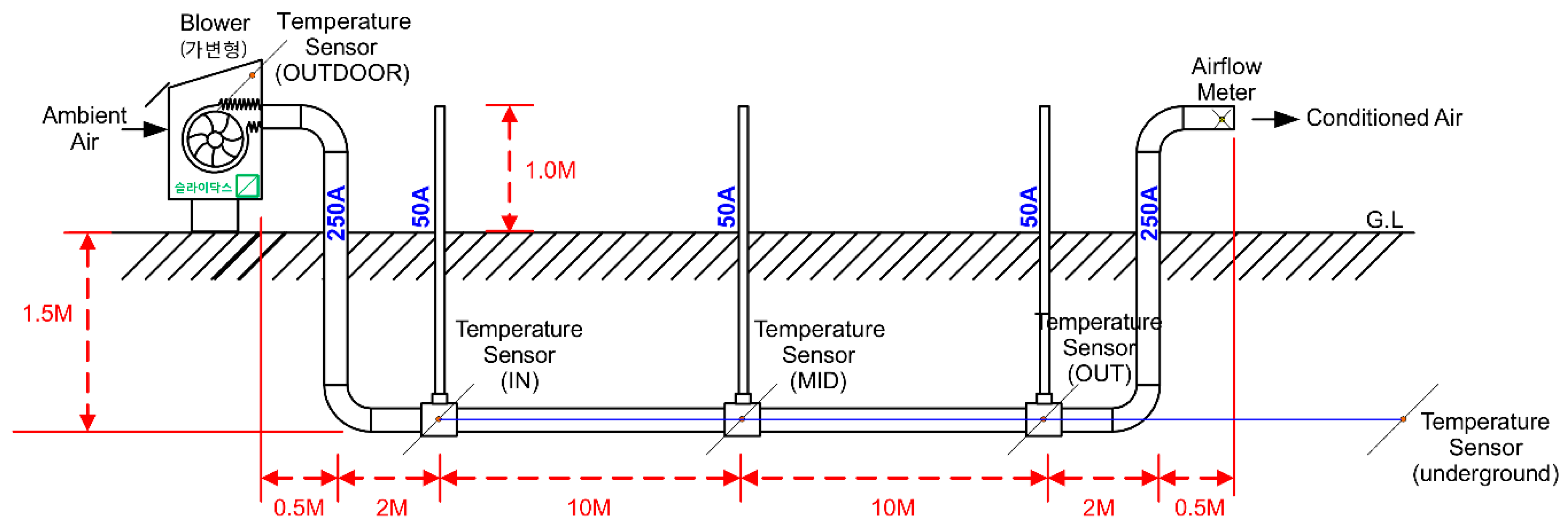
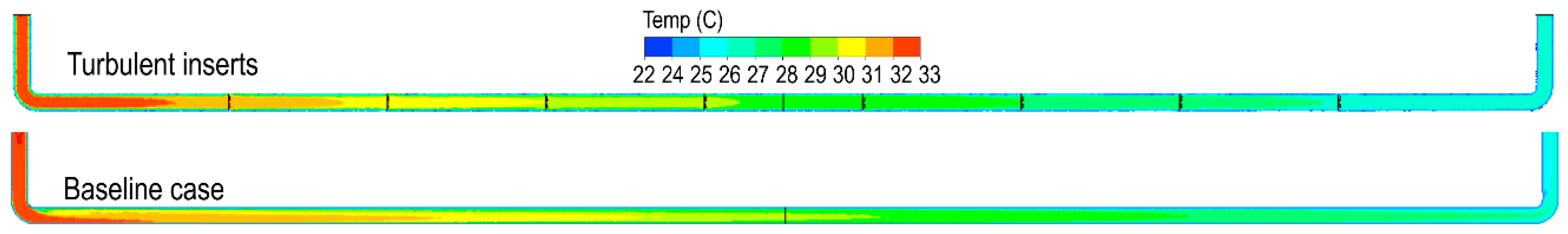
Our simulation experiment consisted of two parts—validation and potential designs. The validation study focused on the two models—baseline and turbulent insert cases. The overall appearance of the baseline case is shown in Figure 1.

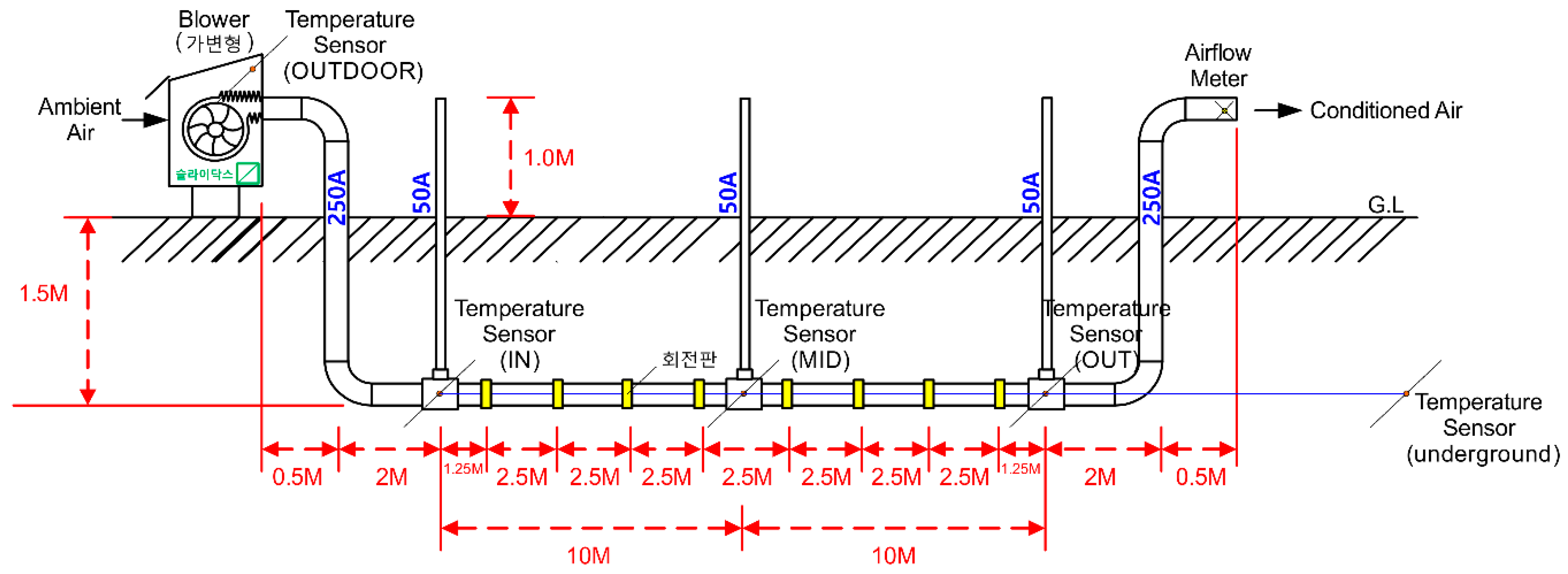
Only the pipe section beneath the ground was included in the computational domain. In other words, the temperatures at the pipe inlet and exit were assumed to be constant and the same at their nearest ground-level boundaries. The turbulent insert case featured the baseline case plus eight turbulent inserts, as shown in Figure 2.

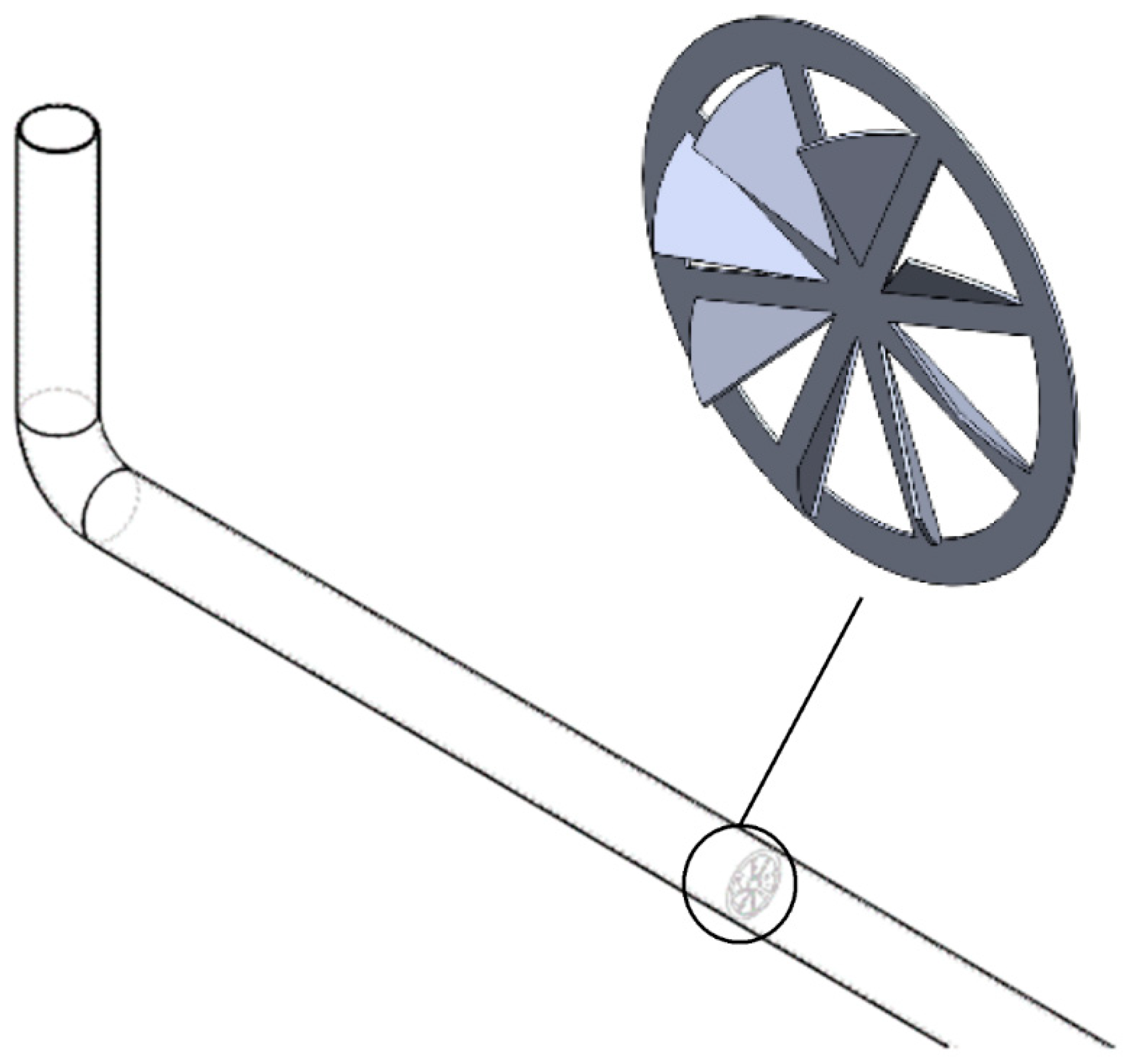
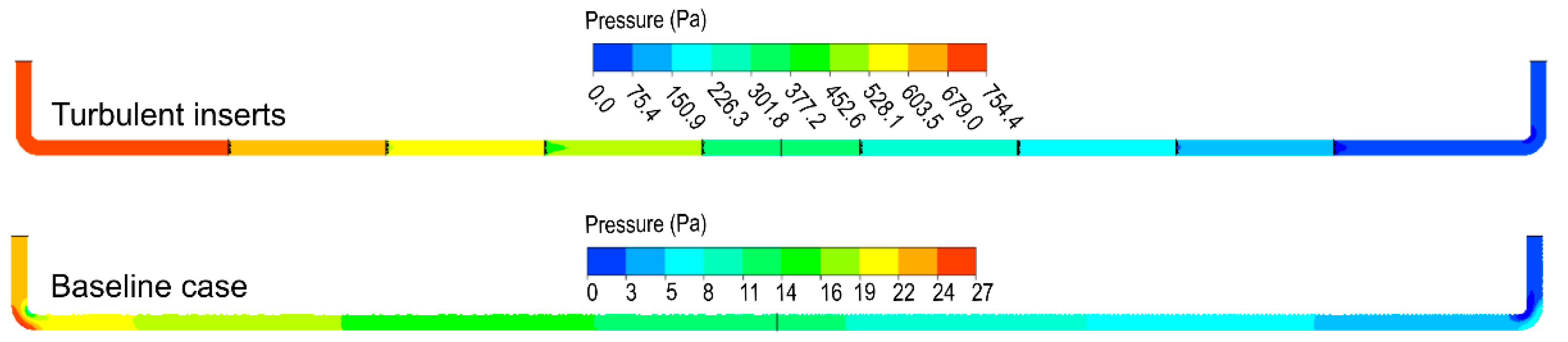
The total computational pipe length for both cases was 88.6 ft (27 m) and the inner diameter of the pipes was 0.82 ft (0.250 m) with a thickness of 0.0279 ft (0.0085 m). In the turbulent insert pipe, the inserts were circular plates with angularly bent fins (Figure 3). These plates were placed 8.2 ft (2.5 m) from each other (Figure 2). There were three temperature sensors placed at 0, 10, and 20 m (Figure 2 and Figure 3). However, only positions 0 and 20 m were monitored in the validation study.

The simulation was performed for four consecutive days corresponding to the experimental data observed during summer in South Korea. The ground and outdoor temperatures are reported in

Table 1. Environmental conditions for the reported data.

Date	Ground Temp (°C)	Outdoor Temp (°C)	Inlet Velocities (m/s)
			Turbulent Insert	Baseline
Aug 13	22.5	33.4	3.53	3.71
Aug 14	22.6	35.4	3.55	3.74
Aug 15	22.7	34.5	3.55	3.72
Aug 16	22.8	32.0	3.67	3.86

. The highest and lowest temperature difference between the ground and outdoors was 12.8 and 9.2 °C, respectively.

A commercial simulation platform was used to perform numerical simulations. For the purpose of this study, a standard k-ε turbulence model with a standard wall function was chosen among the available models (Launder–Spalding wall function, scalable wall functions, non-equilibrium wall functions, enhanced wall treatment, etc.). The model was also chosen due to its stability and simplicity as the turbulent viscosity is calculated in a less complex way. The standard wall function has some weaknesses when applied to complex problems such as high-pressure gradients, buoyancy and complex strains, but in this case, its use is justified as the flow does not experience rapid changes near the pipe inside-walls. For boundary conditions, the velocity inlet and pressure outlet were prescribed at the pipe entrance, respectively. The air entering the pipe was assumed to have an outdoor temperature corresponding to each experimental day (see Table 1). The turbulent intensity was set at 10% as per Basse, N. T. [23] and the Reynolds number and the hydraulic diameter at the inlet was set at 0.82 ft (0.250 m). For the solution method, we used the SIMPLE scheme for pressure-velocity coupling with least-squares cells based on standard pressure. A first-order upwind scheme was applied for momentum, turbulent kinetic energy, and turbulent dissipation rate as its application is sufficient when applied to heat-flow applications with no presence of chemical reactions. However, a second-order upwind scheme was used for the pressure and energy equations. Convergence was reached when the residual was less than 10⁻⁶ for all parameters including continuity, energy, velocities, and the k and ε equations. Convergence also occurred when the pipe outlet temperature stabilized at a constant value.

3. Results

3.1. Grid Independence Study

A mesh independence study was performed for the turbulent insert case (Figure 2). Three different mesh sizes were investigated as shown in

Table 2. Mesh independence study.

Size	Mesh Size	No. of Nodes	No. of Cells	ΔT (°C)
Coarse	1.21 × 10−2–2.42	77,548	402,064	5.81
Medium	6.06 × 10−3–1.21	123,945	672,063	5.94
Fine	3.55 × 10−3–0.71	183,921	1,026,676	5.95

.

An unstructured tetrahedral mesh was used in all mesh generations (Figure 4). The value of Y+ depends on the quality of the mesh and was selected from the range of 30 < Y+ < 500, The temperature difference between the 0 and 20 m measurement points was investigated for changes in mesh size and results showed no significant differences. There was only a 0.13 °C temperature difference at these two points between the coarse and medium mesh sizes. In addition, the difference was only 0.04 °C between the coarse and fine mesh. With such a minimal change in temperature difference, the coarse mesh was selected to adequately represent the flow physics of the air through the pipe model. The pressure drop on each pipe was 755 pa (turbulent plate), 55 pa (spirally corrugated pipe), and 25 pa (baseline), and it was ignored from the point of the mesh independent study.

3.2. Validation Study

The validation study was performed for scenarios with and without turbulent plates. Experiment results were obtained for four days from 13–16 August 2016. The turbulent insert case exhibited slightly closer results to the experiments compared to the baseline case. However, ∆T errors between 0 and 20 m for both the baseline and the turbulent insert scenarios were less than 20%. These results were acceptable considering that all flows were turbulent. Moreover, the local errors at the two locations were less than 5 and 7% for the turbulent insert and baseline case, respectively (

Table 3. Baseline simulation results.

Baseline Case
Date	0 m			20 m			ΔT (20 m–0 m)
	Sim.	Exp.	Diff.	Sim.	Exp.	Diff.	Sim.	Exp.	Diff.
Aug 13	31.5	32.4	3%	27.2	28.0	3%	4.3	4.4	2%
Aug 14	33.0	32.3	2%	28.1	28.2	0%	4.9	4.1	18%
Aug 15	32.4	31.9	2%	27.8	28.0	1%	4.7	3.9	20%
Aug 16	31.0	32.1	4%	26.1	28.0	7%	4.9	4.1	19%

and

Table 4. Turbulent insert simulation results.

Turbulent Insert Case
Date	0 m			20 m			ΔT (20 m–0 m)
	Sim.	Exp.	Diff	Sim.	Exp.	Diff.	Sim.	Exp.	Diff.
Aug 13	32.0	32.7	2%	26.1	26.5	1%	5.81	6.20	6%
Aug 14	34.3	32.5	5%	27.8	27.0	3%	6.40	5.50	16%
Aug 15	33.6	32.2	4%	27.5	26.9	2%	6.06	5.30	14%
Aug 16	31.4	32.5	3%	26.6	27.0	1%	4.75	5.50	14%

)

Figure 5 shows the temperature profiles x = 0 m and x = 20 m. In the turbulent insert case, the temperature was more concentrically uniform at x = 0 m. The hot entering air stream remained at the center of the pipe, and air cooled radially as it moved closer to the pipe wall. Furthermore, the temperature was cooler near the pipe exit (x = 20 m). In the baseline case, temperature exhibited a non-uniform distribution within the cross-sectional profile at x = 0 m. A hotter air stream was located at the bottom of the pipe. The cool temperature layer was also thinner compared to the turbulent insert case. At x = 20 m, the temperature was concentrically distributed and remained higher in the center of the pipe.

The temperature profile in Figure 5 was explained by the following observations. In the turbulent insert case, the downstream plates acted as directional guides for the air to flow more uniformly upstream (Figure 6). Right after the inserted plates, the rotating flow became dominant, which enhanced the heat transfer process from the hot moving air to the cooler ground. In the baseline case, the hot air stream moved undisturbed along the pipe. Because of the downward momentum as air moved through the pipe, air sank towards the bottom of pipe after the first L-turn. This caused the temperature profile to be non-uniform near the inlet (x = 0 m). However, after traveling along the long pipe, the airflow became fully developed and uniform near the exit (x = 20 m, Figure 5).

Figure 7, shows the temperature profile in the middle plane along the pipe for the two scenarios. The turbulent insert case exhibited better heat transfer between the hot moving air inside the pipe and the cool ground. The turbulent plates tend to resist the airflow and create more rotational flows (Figure 6). This kept the hot air moving in good contact with the cooler pipe wall. As a result, the downstream air cooled further as it traveled along the pipe. In contrast, the baseline case exhibited slower cooling as air moved along the pipe. At the same x position, one can see the distinct temperature difference between the two scenarios in Figure 7.

One major drawback of the turbulent insert case was the large pressure decrease. Figure 8 shows the pressure drop across the pipe for both scenarios. After each plate, pressure was significantly reduced. For the baseline case, the pressure drop was only 27 Pa across the pipe. In the next section, we will explore how the reduction in turbulent plates affects the desired temperature drop of the cooled air. Specifically, plate reductions can reduce the pressure drop, which can save power for the inlet fan.

3.3. Parametric Studies

3.3.1. Effects of Turbulent Plate Quantity

In this investigation, the plate quantity was reduced from 8 (original) to 6, 4, and 0 plates. The inlet velocity was kept constant at 3.53 m/s for all cases based on data from 13 August. For the first three cases with 8, 6, and 4 plates, the temperatures at x = 0 m were relatively similar. However, the temperature at x = 20 m increased as the number of plates decreased. As a result, the temperature differences between the two gauged positions also decreased as the number of plates decreased (Figure 10). Finally, in the zero-plate case, the temperature at both x = 0 m and x = 20 m was lower compared to cases with inserted plates (Figure 9).

The temperature differences between x = 0 m and x = 20 m for various plate quantities are plotted in Figure 10. We observed a decrease in cooling temperature as the number of plates decreased. In addition, we plotted the pressure drop for each case. By reducing two plates from eight to six, temperature difference decreased by only 0.63 °C. However, there was a big gap in pressure drop. Temperature differences between the four plates and zero plates cases were very similar. Thus, it is not recommended to use four plates in practice. Instead, either 6 or 0 plates is preferred depending on the amount of air cooling required before reaching the residential house.

3.3.2. Effects of Different Pipe Materials

In Figure 11, the effects of different materials on temperatures at two locations, x = 0 m and x = 20 m are shown.

Table 5. Material properties.

Material Properties
	PVC	PC	PE	Steel (for All Inserts)
Density (kg/m3)	1450	1200	960	8050
Thermal Conductivity (W/m-K)	0.28	0.25	0.33	16.27
Specific Heat (J/kg-K)	900	1300	1850	502.48

shows the properties of the three materials investigated.

Overall, the temperatures at x = 0 m for all cases were nearly identical. However, the difference in the material had a small effect on downstream air temperature (x = 20 m). Figure 12 shows the temperature difference between the two locations for three different materials—polyvinyl chlorine (PVC), polycarbonate (PC), and polyethylene (PE). The temperature difference was lowest in the PC case and highest in the PE case, though these differences were not significant.

3.4. Pipe Type Exploration

In this section, three additional pipe types are detailed—corrugated, helical insert, and spirally corrugated pipes. The temperature drops between the two gauged positions are reported in

Table 6. Results for different pipe types using conditions from 13 August 2016.

Pipe Type	Toutdoor	Tx = 0 m (°C)	Tx = 20 m (°C)	ΔT20 m–0 m (°C)	ΔToutdoor – 20 m (°C)	Vinlet (m/s)
Baseline	33.4	32.0	27.4	4.6	6.0	3.71
Turbulent Insert	33.4	32.0	26.1	5.8	7.3	3.53
Corrugated	33.4	31.9	27.2	4.8	6.2	3.71
Helical Insert	33.4	31.5	26.5	5.0	6.9	3.71
Spirally Corrugated	33.4	30.9	25.7	5.2	7.7	3.71

. These results were obtained using the boundary conditions for 13 August 2016 (Table 1). The inlet velocity used for the corrugated, helical insert and spirally corrugated pipe cases was the same as the baseline case (3.71 m/s), while the turbulent insert case inlet velocity was kept at 3.53 m/s.

From Table 6, the baseline case had the highest temperature at x = 20 m, resulting in the lowest temperature drop (6 °C). The turbulent insert case featured the best temperature drop at x = 20 m compared to the entering air temperature (7.3 °C) and the air temperature at x = 0 m (5.8 °C). The corrugated pipe case had a slightly better temperature decrease of 6.2 °C and 4.8 °C with respect to the entering and 0 m air temperature, respectively. The helical insert case had a second-best temperature drop when compared to the outside air (6.9 °C), although the temperature at 20 m was only 5 °C. Finally, the spirally corrugated pipe case exhibited the best improvement in temperature drop when compared to the outside air and second-best at 20 m. Figure 13 clearly reflects these temperature drop comparisons for the five investigated cases.

Figure 14 and Figure 15 show the temperature and pressure profiles of the five studied cases. Although the turbulent insert case exhibited a reasonably good temperature drop along the linear pipe, its major drawback was the high-pressure drop (755 Pa), which caused extensive amounts of electrical energy to be consumed in the blower. The spirally corrugated pipe, however, demonstrated the best temperature drop (7.7 °C) without inducing a large pressure drop (only 55 Pa). The baseline case had the lowest pressure drop due to a lack of obstructions within the pipe. Taking temperature and pressure drops into consideration, the spirally corrugated pipe case stood out as the preferred option for practical use. However, more data is required for validation.

4. Design Guideline of a GAHX for an AWHP

In this section, we demonstrate how to select the most optimal pipe design in terms of type, material, and size. From the previous section, the spirally corrugated pipe was determined to be the most desirable. In the following example, a calculation is performed for a typical office space with a total floor area of 147 m² (1581 ft²). It is desirable for an AWHP system to achieve a coefficient of performance (COP) of approximately 3.0. According to Perko et al. [24], an average-sized space (186–223 m²) requires a thermal power of 10.6 kW to 11.4 kW, depending on climate conditions. In the worst-case scenario, a small area of 186 m² requires a heating power of 11.4 kW. The ratio (r) of floor area per kilowatt can then be calculated as:

$$\mathrm{r}=\frac{\mathrm{A}}{\mathrm{P}}=\frac{186 {\mathrm{m}}^2}{11.4 \mathrm{kW}}=16.32 \frac{{\mathrm{m}}^2}{\mathrm{kW}}$$

(1)

where, r is the floor area ratio per kW, A is floor area, and P is the required heating power.

The thermal power at the condenser was then calculated from the actual floor area of 147 m² using:

$${\mathrm{Q}}_{\mathrm{condenser}}=\frac{{\mathrm{A}}_{\mathrm{office}}}{\mathrm{r}}\approx 9 \mathrm{kW}$$

(2)

The target COP for the AWHP was set as 3.0. Therefore, the power required from the compressor was:

$$\mathrm{COP}=\frac{{\mathrm{Q}}_{\mathrm{out}}}{{\mathrm{W}}_{\mathrm{e} \mathrm{in}}}=\frac{{\mathrm{Q}}_{\mathrm{condenser}}}{{\mathrm{Q}}_{\mathrm{conpressor}}}$$

(3)

$${\mathrm{Q}}_{\mathrm{compressor}}=\frac{{\mathrm{Q}}_{\mathrm{condenser}}}{\mathrm{COP}}=\frac{9 \mathrm{kW}}{3}=3 \mathrm{kW}$$

(4)

The required thermal power from air flowing through the buried pipe was therefore calculated as:

$${\mathrm{Q}}_{\mathrm{geothermal}}={\mathrm{Q}}_{\mathrm{condenser}}-{\mathrm{Q}}_{\mathrm{compressor}}=9 \mathrm{kW}-3 \mathrm{kW}=6 \mathrm{kW}$$

(5)

In addition, the spirally corrugated pipe had a total length of 28 m. Therefore, heat extraction from the ground source was calculated as:

$$\begin{array}{ll}{\mathrm{R}}_{\mathrm{extract}}& =\frac{{\mathrm{Q}}_{\mathrm{pipe}}}{{\mathrm{l}}_{\mathrm{pipe},\mathrm{calculated}}}=\frac{{\mathrm{C}}_{\mathrm{p}\mathrm{air}}\times {\dot{m}}_{\mathrm{air}}\times (T_{20\mathrm{m}}-T_{0\mathrm{m}})}{{\mathrm{l}}_{\mathrm{pipe},\mathrm{calculated}}}\\ & =\frac{1005\frac{\mathrm{J}}{\mathrm{kg}℃}\times 0.223\frac{\mathrm{kg}}{\mathrm{s}}\times 5.2℃}{20\mathrm{m}}=58.25\mathrm{W}/\mathrm{m}\end{array}$$

(6)

The target COP 3.0 resulted in a required thermal power from the underground pipe of 6 kW. From here, the total pipe length was calculated using:

$${\mathrm{l}}_{\mathrm{pipe}, \mathrm{calculated}}=\frac{{\mathrm{Q}}_{\mathrm{geothermal}}}{{\mathrm{R}}_{\mathrm{extract}}}=\frac{6000\mathrm{W}}{58.25\mathrm{W}/\mathrm{m}}\approx 103 \mathrm{m}$$

(7)

Finally, the actual pipe length including the U-shape section to the ground surface was calculated by adding an extra 8 m:

$${\mathrm{l}}_{\mathrm{pipe},\mathrm{final}}=103\mathrm{m}+8 \mathrm{m}=111 \mathrm{m}$$

(8)

The final optimal pipe design is summarized in

Table 7. Design input and output of the office space calculation for a target COP of 3.0.

Design Input	Design Output
${\mathrm{A}}_{\mathrm{office}}=147{\mathrm{m}}^2\left(1581{\mathrm{ft}}^2\right)$	${\mathrm{l}}_{\mathrm{pipe},\mathrm{calculated}}=103\mathrm{m}$
${\mathrm{Q}}_{\mathrm{condenser}}=9\mathrm{kW}$	${\mathrm{l}}_{\mathrm{pipe},\mathrm{final}}=111\mathrm{m}$
${\mathrm{Q}}_{\mathrm{geothermal}}=6\mathrm{kW}$	${\phi }_{\mathrm{pipe}}=0.25 \mathrm{m}$
${\mathrm{Q}}_{\mathrm{compressor}}=3\mathrm{kW}$
$\mathrm{COP}=3.0$
${\mathrm{l}}_{\mathrm{pipe},\mathrm{total}}=28\mathrm{m}$
${\mathrm{l}}_{\mathrm{pipe},\mathrm{calculated}}=20\mathrm{m}$
$T_{20m}-T_{0m}=5.2 ℃$
${\mathrm{v}}_{\mathrm{air}}=3.71\mathrm{m}/\mathrm{s}$
$\dot{m}=0.224\mathrm{kg}/\mathrm{s}$
$T_{\mathrm{ground}}=22.5℃$
$T_{\mathrm{ambient}}=33.4℃$
${\rho }_{\mathrm{air}}=1.225\mathrm{kg}/{\mathrm{m}}^3$
${\mathrm{C}}_{\mathrm{p},\mathrm{air}}=1.005\mathrm{kJ}/\mathrm{kg}.\mathrm{K}$
${\mathrm{R}}_{\mathrm{extract}}=58.25\mathrm{W}/\mathrm{m}$

. This design yielded a maximum 6 kW in thermal power on top of the 3-kW power required by the compressor. This allowed a COP of 3.0 for the AWHP system used to heat up an office space of 147 m² (1581 ft²) in winter.

5. Conclusions

In this paper, the GAHX was studied to yield the best design for a maximum temperature change and minimum pressure drop. The smooth pipe and turbulent insert case were validated against data obtained during the summer in South Korea. Results demonstrated good agreement between the simulated and experimental results. Additional work was performed to explore various design alternatives to improve temperature decrease. From the simulations, the turbulent insert case exhibited the best improvement in terms of temperature drop, yet had the highest pressure drop across the pipe. However, the spirally corrugated pipe demonstrated the best temperature drop (7.7 °C) with a small pressure drop of 55 Pa. Therefore, the spirally corrugated pipe was determined to be the optimal design. An example calculation for an average office space was then provided as a guideline to select the proper pipe size for a spirally corrugated pipe. It was calculated that a 111 m pipe length with a diameter of 250 mm can provide 6 kW of thermal power, which resulted in a COP of 3.0 for the AWHP system used in the office space. In our future work, we will conduct sensitivity analysis with turbulent intensity 5% to 15%. A mesh independent study on pressure drop and application of swept mesh will be considered on the meshing process to improve the model accuracy. We will conduct additional tests and experiments on the new design AWHP coupled with the GAHX based on the results of this study.

References

1. Yildiz, A.; Ozgener, O.; Ozgener, L. Exergetic performance assessment of solar photovoltaic cell (PV) assisted earth to air heat exchanger (EAHE) system for solar greenhouse cooling. Energy Build. 2011, 43, 3154–3160. [Google Scholar] [CrossRef]
2. Lee, K.; Ryu, N.; Kang, E.; Lee, E. Ground air heat exchanger design and analysis for air source heat pump. Korea Soc. Geotherm. Energy Eng. 2016, 12, 1–6. [Google Scholar] [CrossRef]
3. Muehleisen, R.T. Simple design tools for earth-air heat exchangers. Proc. SimBuild 2012, 5, 723–730. [Google Scholar]
4. Hollmuller, P.; Lachal, B.M. TRNSYS Compatible Moist Air Hypocaust Model; Centre universitaire d’étude des problèmes de l’énergie, University of Geneve: Geneva, Switzerland, 1998. [Google Scholar]
5. Lee, K.H.; Strand, R.K. The cooling and heating potential of an earth tube system in buildings. Energy Build. 2008, 40, 486–494. [Google Scholar] [CrossRef]
6. Vlad, G.E.; Ionescu, C.; Necula, H.; Badea, A. Thermoeconomic design of an earth to air heat exchanger used to preheat ventilation air in low energy buildings. In Proceedings of the International Conference on Energy, Environment, Entrepreneurship, and Innovation, Lanzarote, Spain, 27–29 May 2011; pp. 11–16. [Google Scholar]
7. De Paepe, M.; Janssens, A. Thermo-hydraulic design of earth-air heat exchangers. Energy Build. 2003, 35, 389–397. [Google Scholar] [CrossRef]
8. Rehau Ecoair Ground-Air Heat Exchanger System. Available online: http://www.rehau.com (accessed on 20 May 2019).
9. Euyjoon, L.; Eunchul, K.; Kwangseob, L.; Eviguaniy, E.; Libing, Y.; Mohammed, G. Kier-Canmet ENERGY Joint Study for CO2 free Trigenration System Development based on GAHX Report; Korea Institute of Energy Research: Daejeon, South Korea, 2017. [Google Scholar]
10. Vikas, B.; Rohit, M.; Ghanshyam, D.A.; Jyotirmay, M. Performance analysis of earth–pipe–air heat exchanger for summer cooling. Energy Build. 2010, 42, 645–648. [Google Scholar]
11. Viorel, B. Simple and accurate model for the ground heat exchanger of a passive house. Renew. Energy 2007, 32, 845–855. [Google Scholar]
12. Huijun, W.; Shengwei, W.; Dongsheng, Z. Modelling and evaluation of cooling capacity of earth–air–pipe systems. Energy Convers. Manag. 2007, 48, 1462–1471. [Google Scholar]
13. Zukowski, M.; Topolanska, J. Comparison of thermal performance between tube and plate ground-air heat exchangers. Renew. Energy 2018, 115, 697–710. [Google Scholar] [CrossRef]
14. Cuny, M.; Lin, J.; Siroux, M.; Magnenet, V.; Fond, C. Influence of coating soil types on the energy of earth-air heat exchanger. Energy Build. 2018, 158, 1000–1012. [Google Scholar] [CrossRef]
15. Amanowicz, Ł. Influence of geometrical parameters on the flow characteristics of multi-pipe earth-to-air heat exchangers–experimental and CFD investigations. Appl. Energy 2018, 226, 849–861. [Google Scholar] [CrossRef]
16. Zhao, Y.; Li, R.; Ji, C.; Huan, C.; Zhang, B. Parametric study and design of an earth-air heat exchanger using model experiment for memorial heating and cooling. Appl. Therm. Eng. 2019, 148, 838–845. [Google Scholar] [CrossRef]
17. Noorollahi, Y.; Saeidi, R.; Mohammadi, M.; Amiri, A.; Hosseinzadeh, M. The effects of ground heat exchanger parameters changes on geothermal heat pump performance—A review. Appl. Therm. Eng. 2018, 129, 1645–1658. [Google Scholar] [CrossRef]
18. Agrawal, K.K.; Yadav, T.; Misra, R.; Agrawal, G.D. Effect of soil moisture contents on thermal performance of earth-air-pipe heat exchanger for winter heating in arid climate: In situ measurement. Geothermics 2019, 77, 12–23. [Google Scholar] [CrossRef]
19. Agrawal, K.K.; Yadav, T.; Misra, R.; Agrawal, G.D. The state of art on the applications, technology integration, and latest research trends of earth-air-heat exchanger system. Geothermics 2019, 82, 34–50. [Google Scholar] [CrossRef]
20. Mahdavi, S.; Sarhaddi, F.; Hedayatizadeh, M. Energy/exergy based-evaluation of heating/cooling potential of PV/T and earth-air heat exchanger integration into a solar greenhouse. Appl. Therm. Eng. 2019, 149, 996–1007. [Google Scholar] [CrossRef]
21. Ali, S.; Muhammad, N.; Amin, A.; Sohaib, M.; Basit, A.; Ahmad, T. Parametric Optimization of Earth to Air Heat Exchanger Using Response Surface Method. Sustainability 2019, 11, 3186. [Google Scholar] [Green Version]
22. Li, H.; Ni, L.; Liu, G.; Zhao, Z.; Yao, Y. Feasibility study on applications of an Earth-air Heat Exchanger (EAHE) for preheating fresh air in severe cold regions. Renew. Energy 2019, 133, 1268–1284. [Google Scholar] [CrossRef]
23. Basse, N.T. Turbulence intensity and the friction factor for smooth-and rough-wall pipe flow. Fluids 2017, 2, 30. [Google Scholar] [CrossRef]
24. Perko, J.; Dugec, V.; Topic, D.; Sljivac, D.; Kovac, Z. Calculation and design of the heat pumps. In Proceedings of the 2011 3rd International Youth Conference on Energetics (IYCE), Leiria, Portugal, 7–9 July 2011; pp. 1–7. [Google Scholar]
Figure 1. Baseline case.
Energies 12 04047 g001
Figure 2. Turbulent insert case.
Energies 12 04047 g002
Figure 3. Turbulent insert pipe.
Energies 12 04047 g003
Figure 4. Mesh generation.
Energies 12 04047 g004
Figure 5. Temperature profiles at x = 0 m and x = 20 m for the baseline and turbulent insert cases.
Energies 12 04047 g005
Figure 6. Streamlines originating from the pipe inlet (a) with turbulent insert, (b) baseline
Energies 12 04047 g006
Figure 7. Temperature profile in the middle plane along the pipe for the two scenarios.
Energies 12 04047 g007
Figure 8. Pressure drop profile in the middle plane along the pipe for two scenarios.
Energies 12 04047 g008
Figure 9. The effect of fins on the temperature of the two locations (0 and 20 m) at a vinlet of 3.53 m/s.
Energies 12 04047 g009
Figure 10. The temperature differences between x = 0 m and x = 20 m for various plate quantities.
Energies 12 04047 g010
Figure 11. The effect of different materials on temperatures at 0 m and 20 m, at vinlet = 3.53 m/s.
Energies 12 04047 g011
Figure 12. The temperature difference between x = 0 m and x = 20 m for different materials.
Energies 12 04047 g012
Figure 13. Temperature drop for the five investigated pipes.
Energies 12 04047 g013
Figure 14. Temperature profile in the middle plane for five investigated pipes.
Energies 12 04047 g014
Figure 15. Pressure drop profile in the middle plane for five investigated pipes.
Energies 12 04047 g015