State-Of-Charge Estimation for Lithium-Ion Battery Using Improved DUKF Based on State-Parameter Separation

Abstract
:
1. Introduction
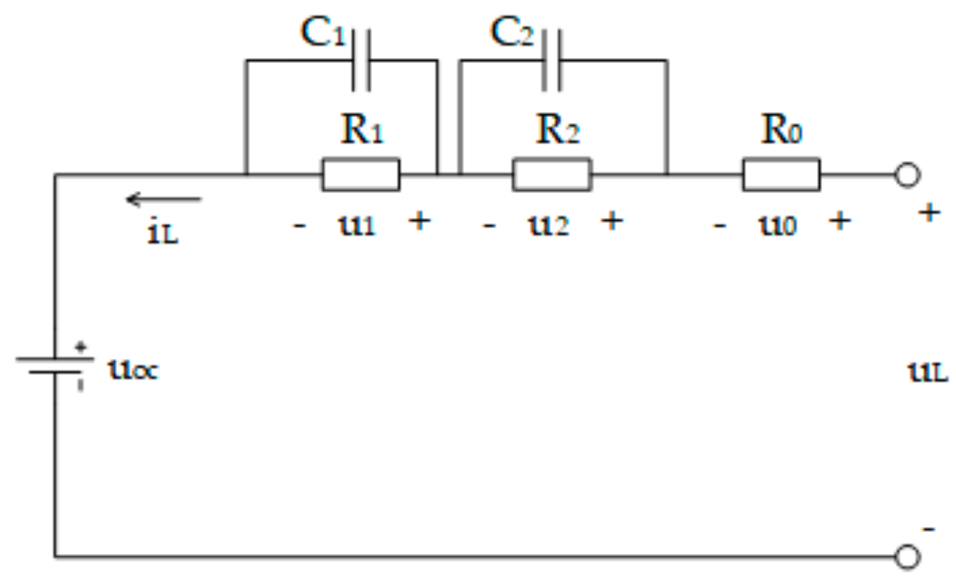
2. Battery Model and Off-Line Parameter Identification Method
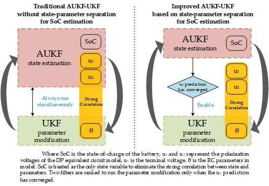
3. Implementation of the State-Parameter Separated IAUKF-UKF
3.1. State-Parameter Separated Equation for Dynamic Battery Model
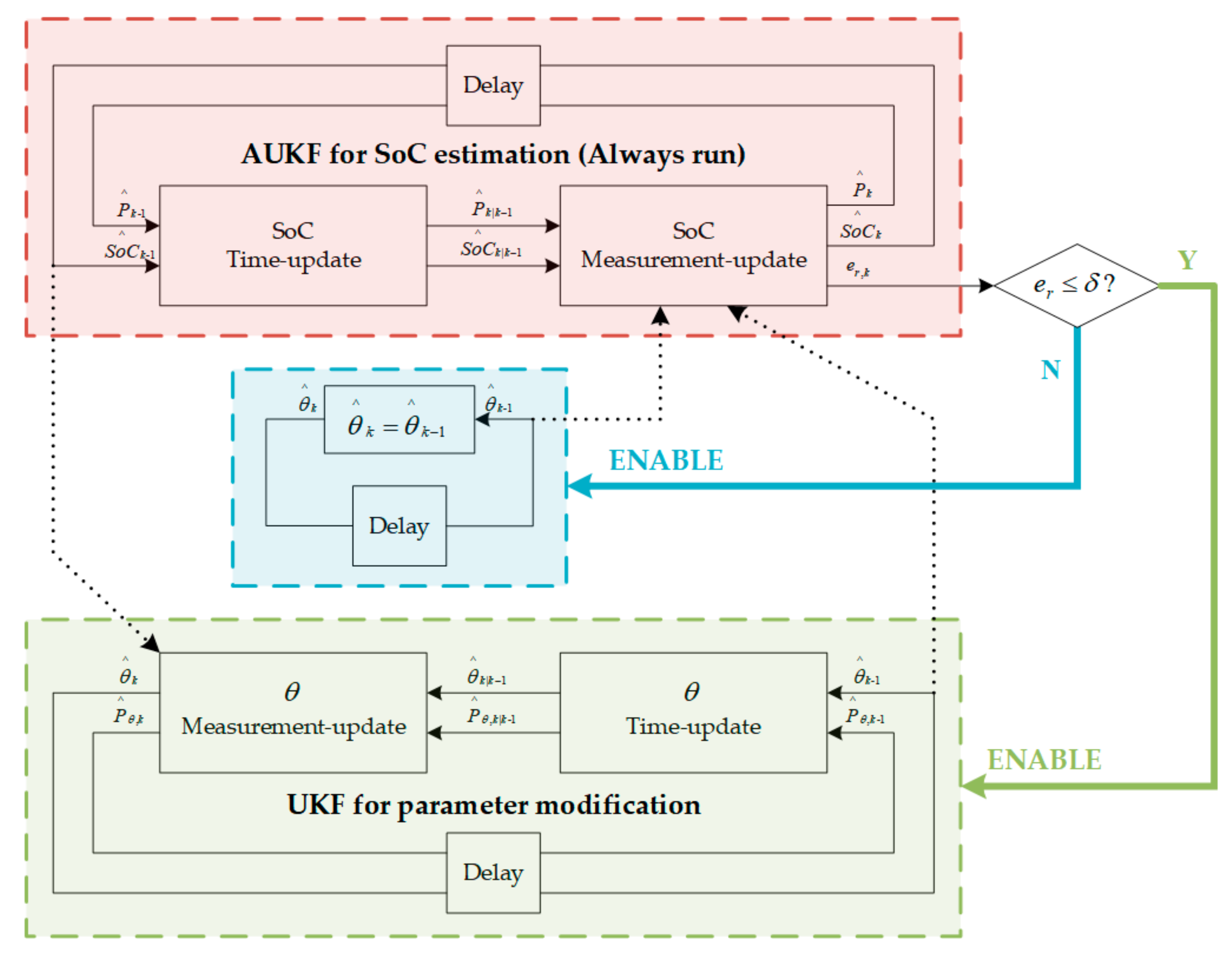
3.2. Improved Dual-Unscented Kalman Filter (IDUKF) Algorithm
4. Experiments
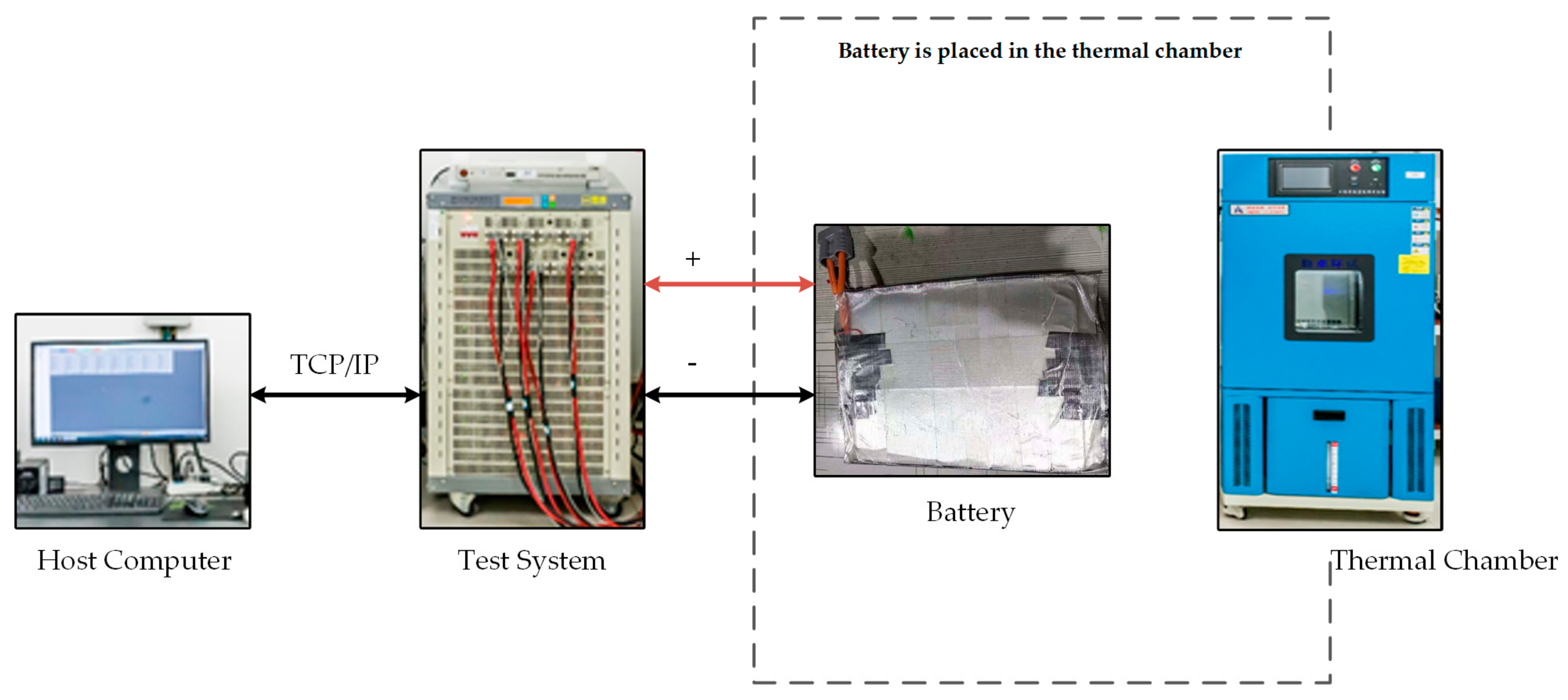
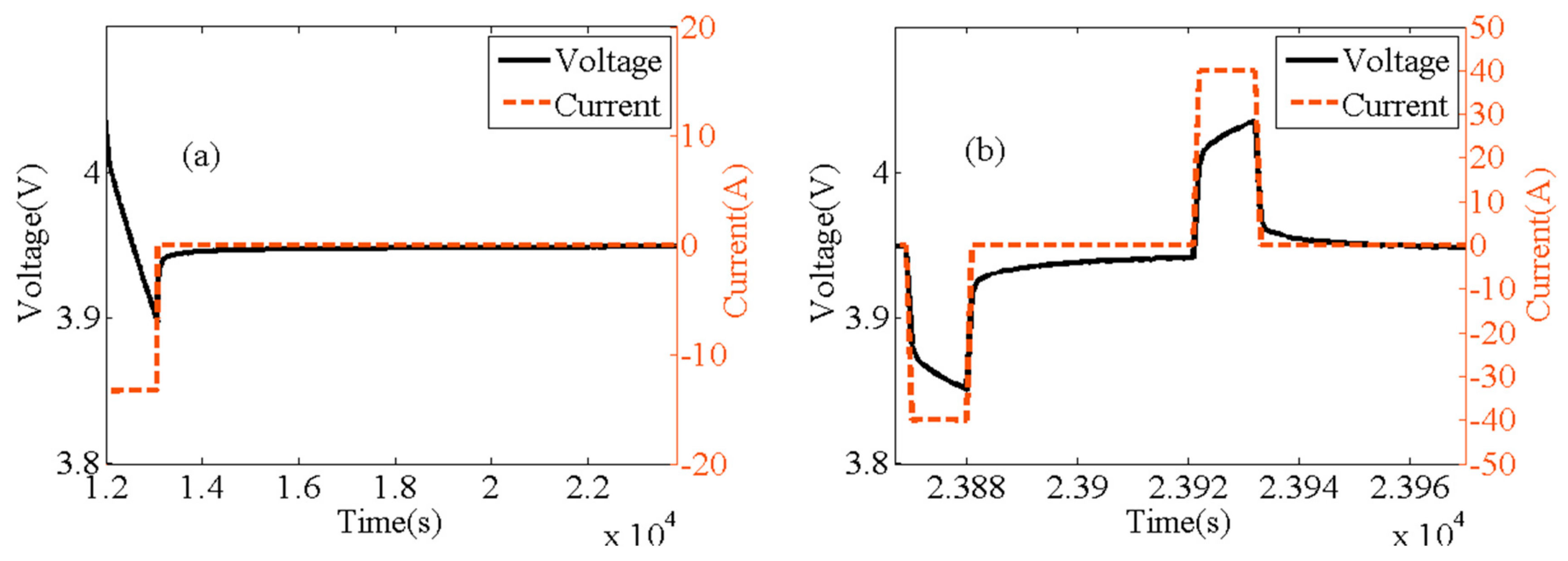
4.1. Experimental Bench
4.2. Experimental Methods
5. Results and Discussion
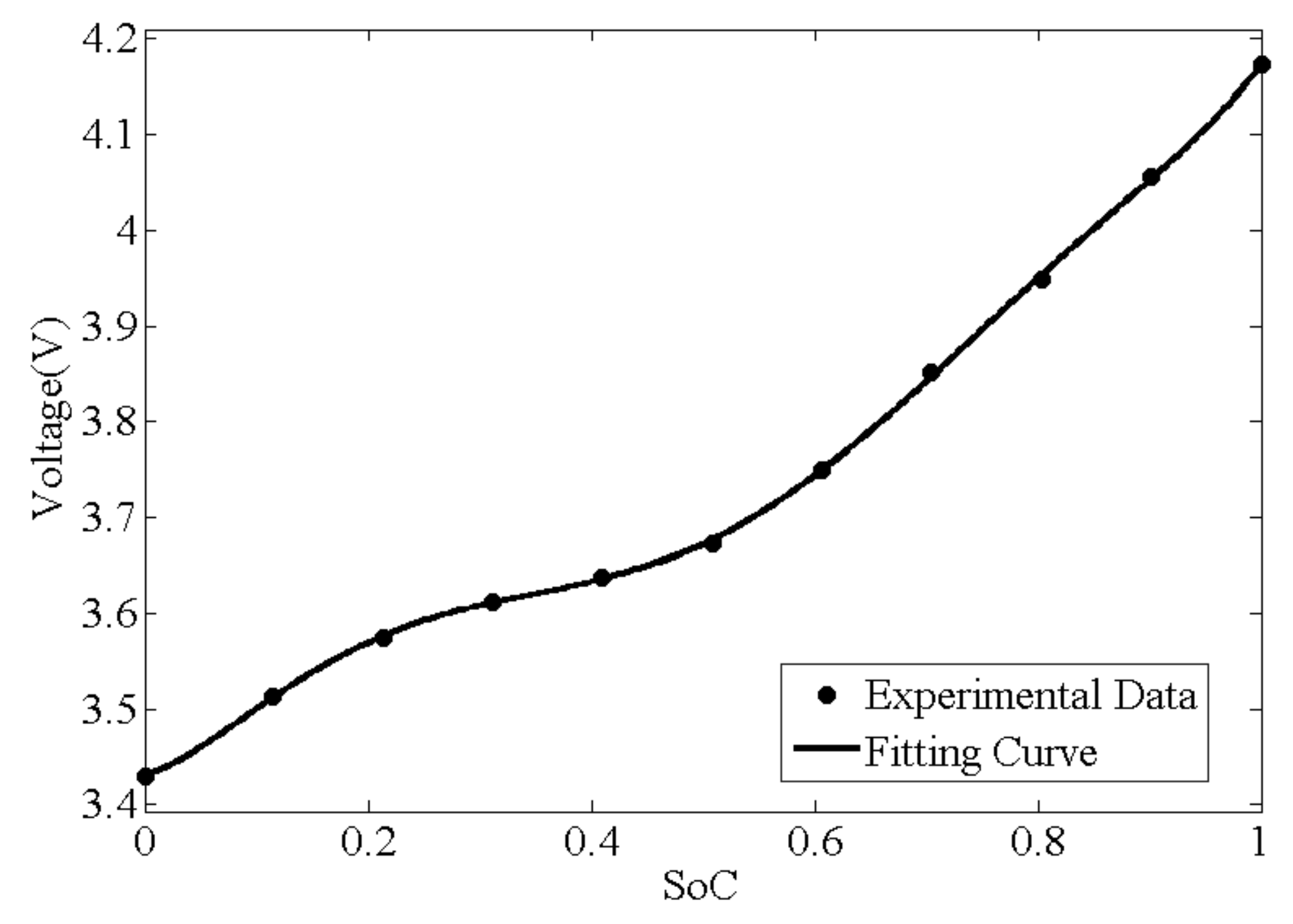
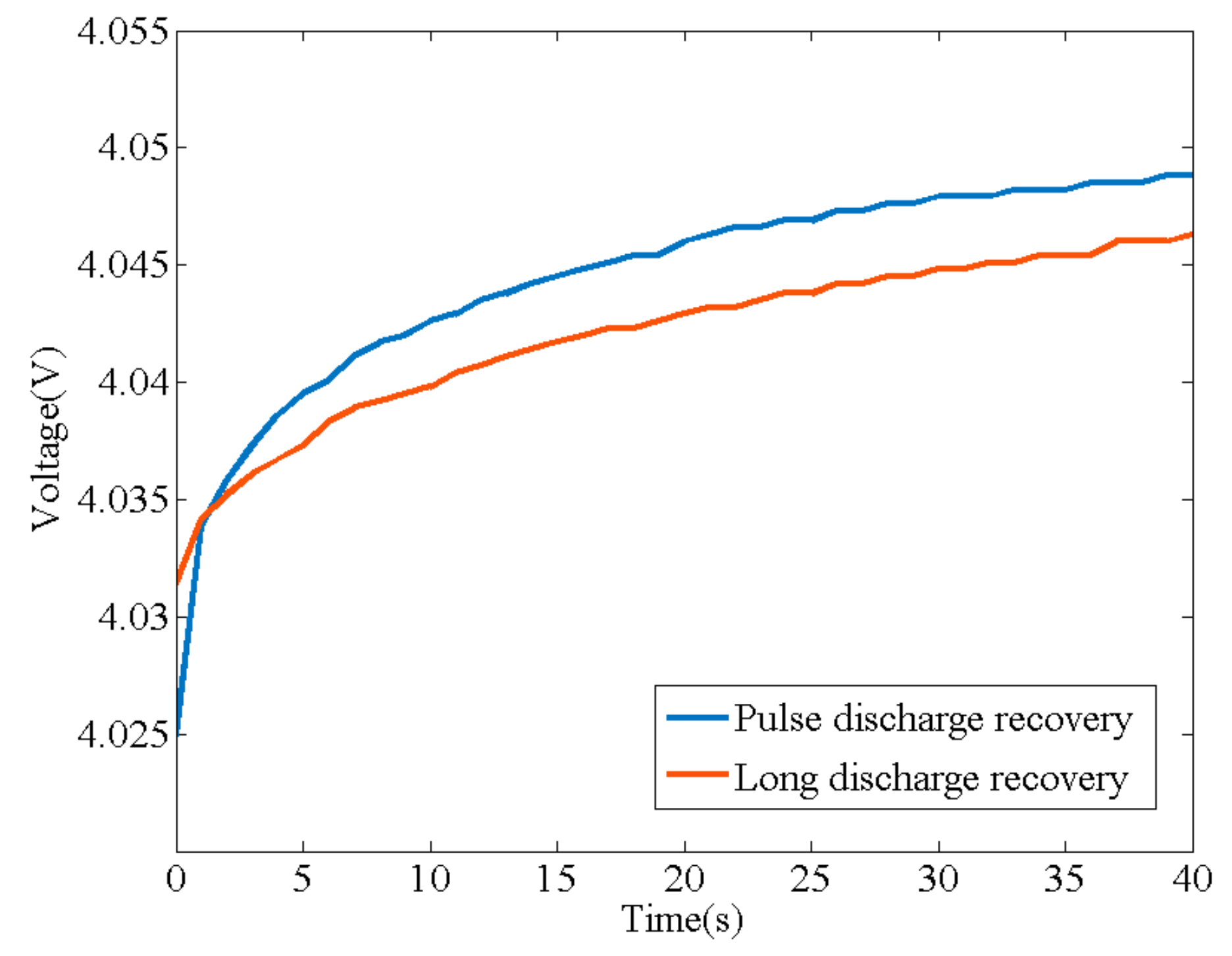
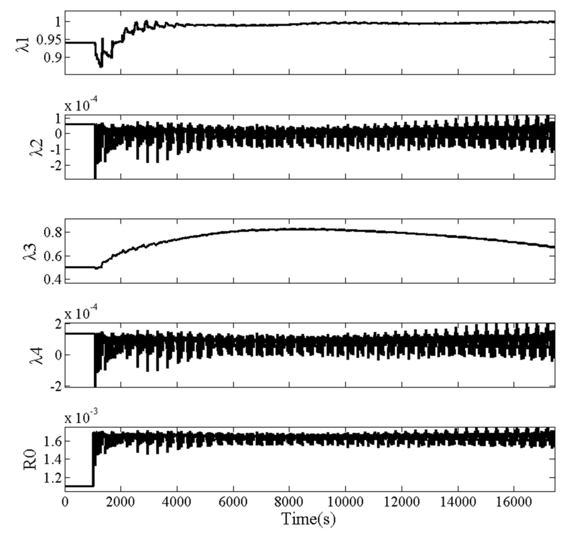
5.1. Off-Line Parameters Identification Results
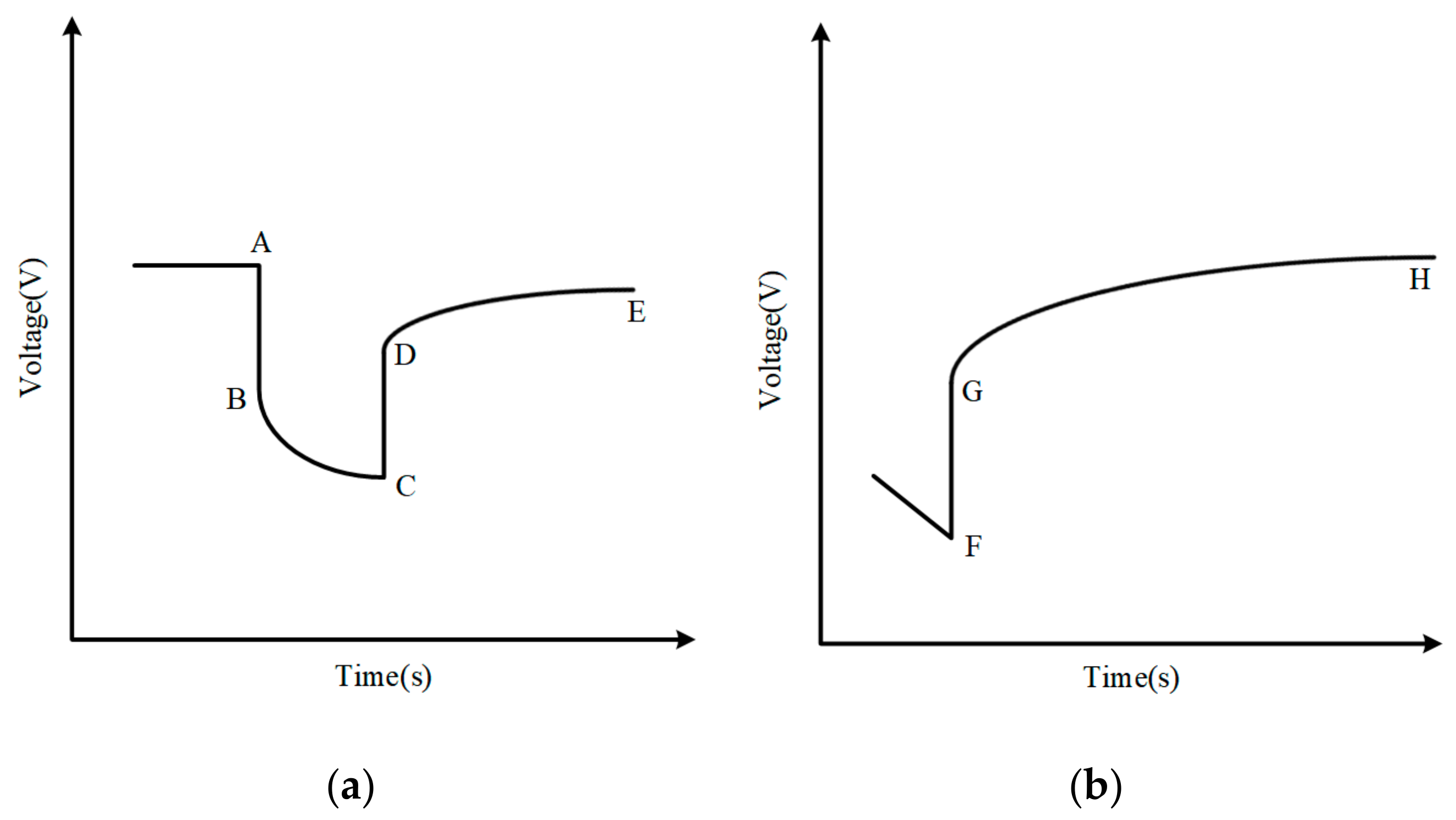
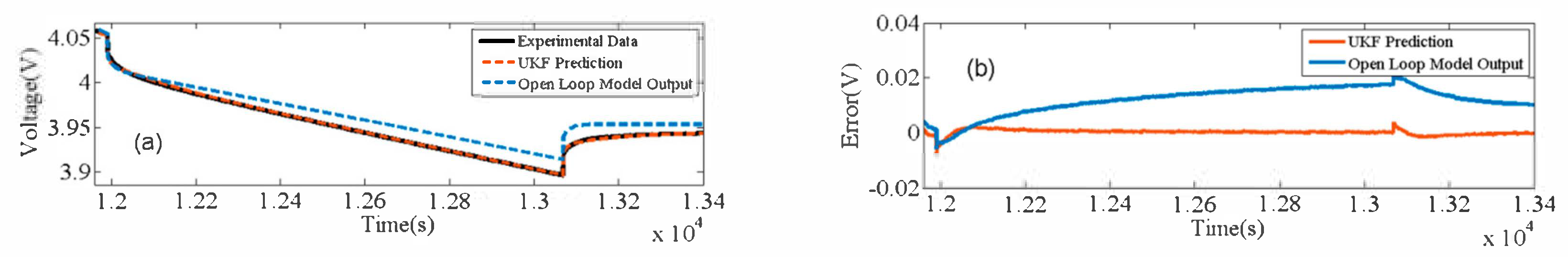
5.2. Advance Explanation of Model Accuracy Evaluation Method
5.3. Comparative Analysis of Algorithms
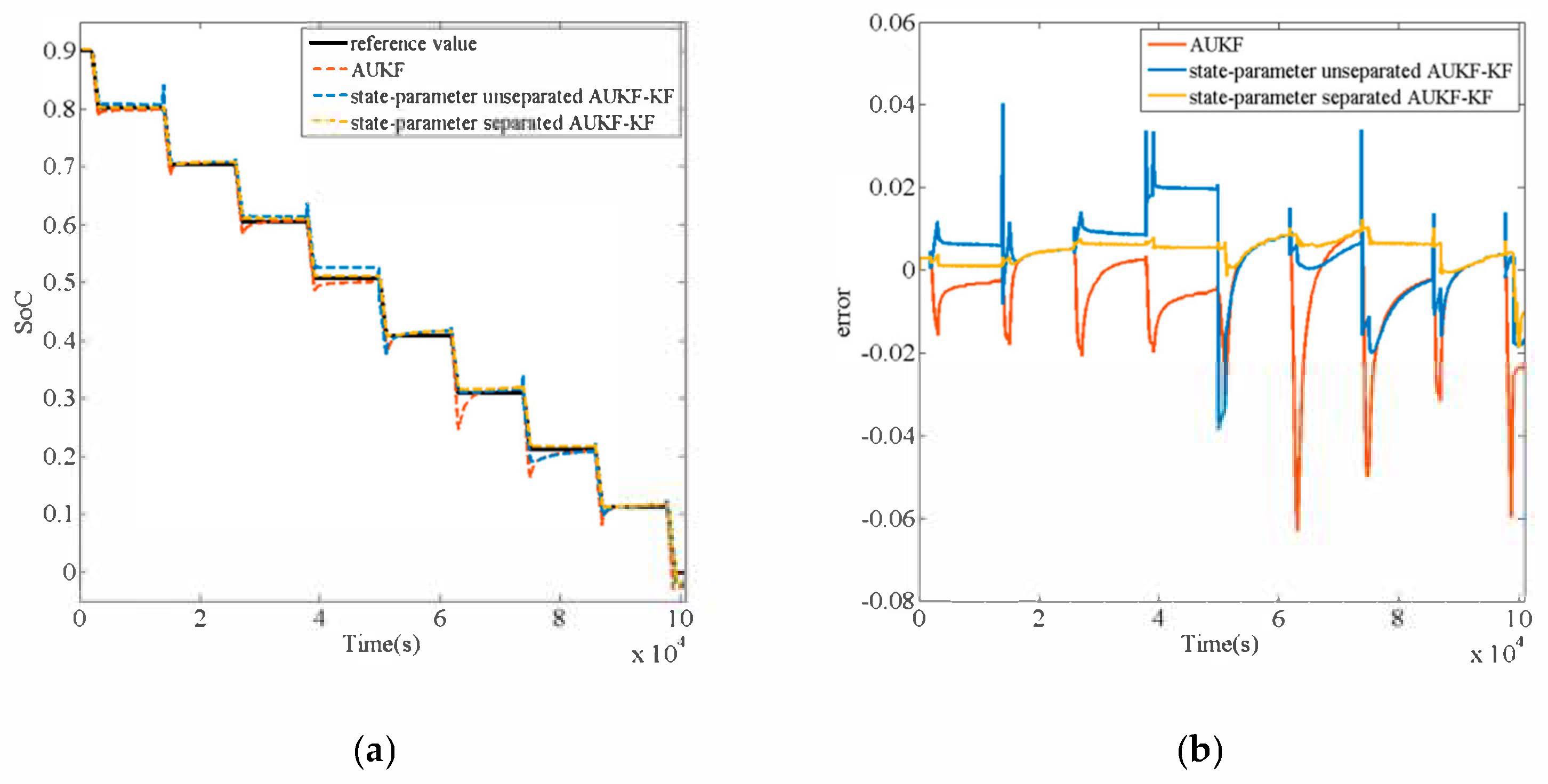
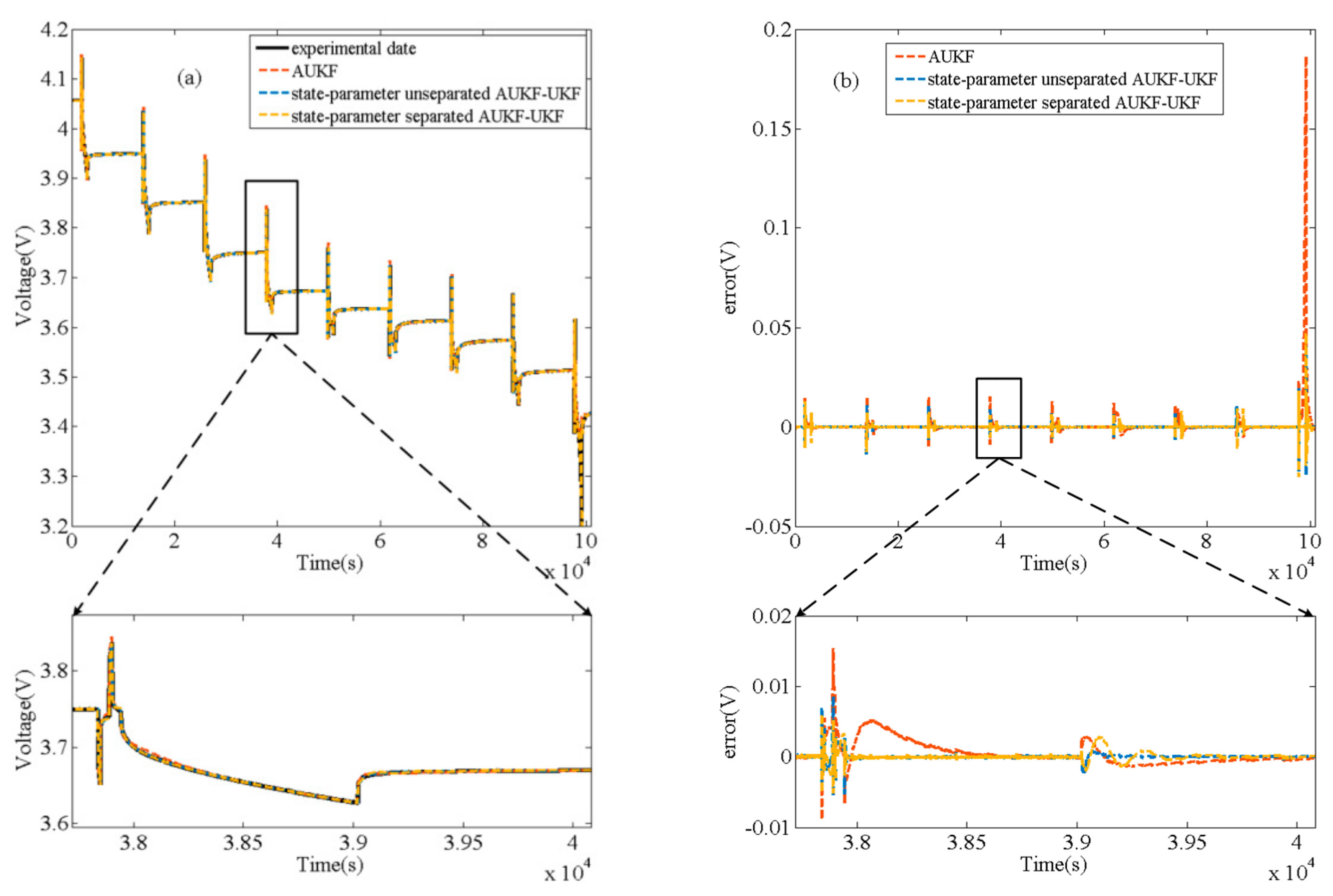
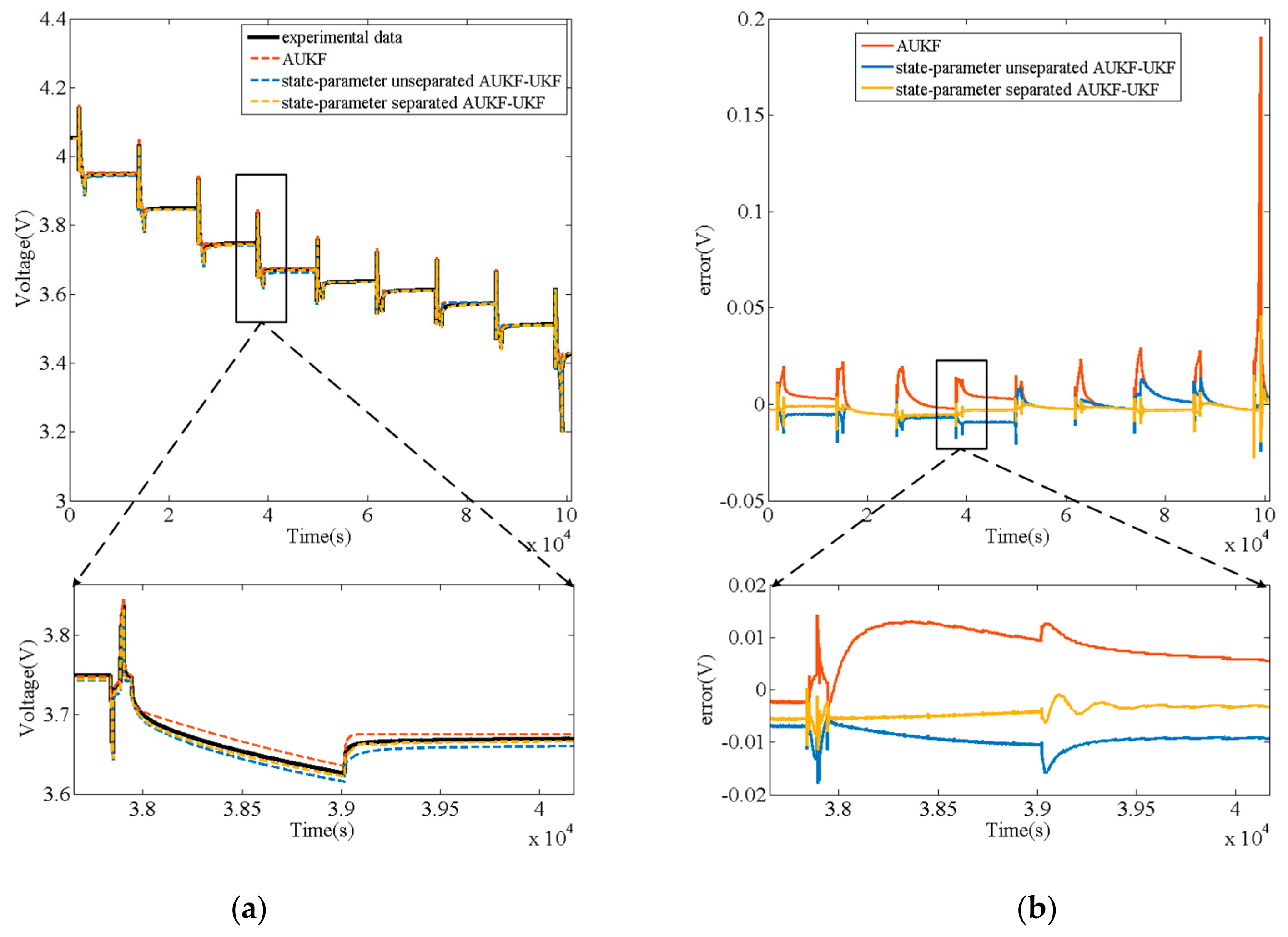
5.3.1. Comparison of SoC Estimation and Parameter Modification Accuracy
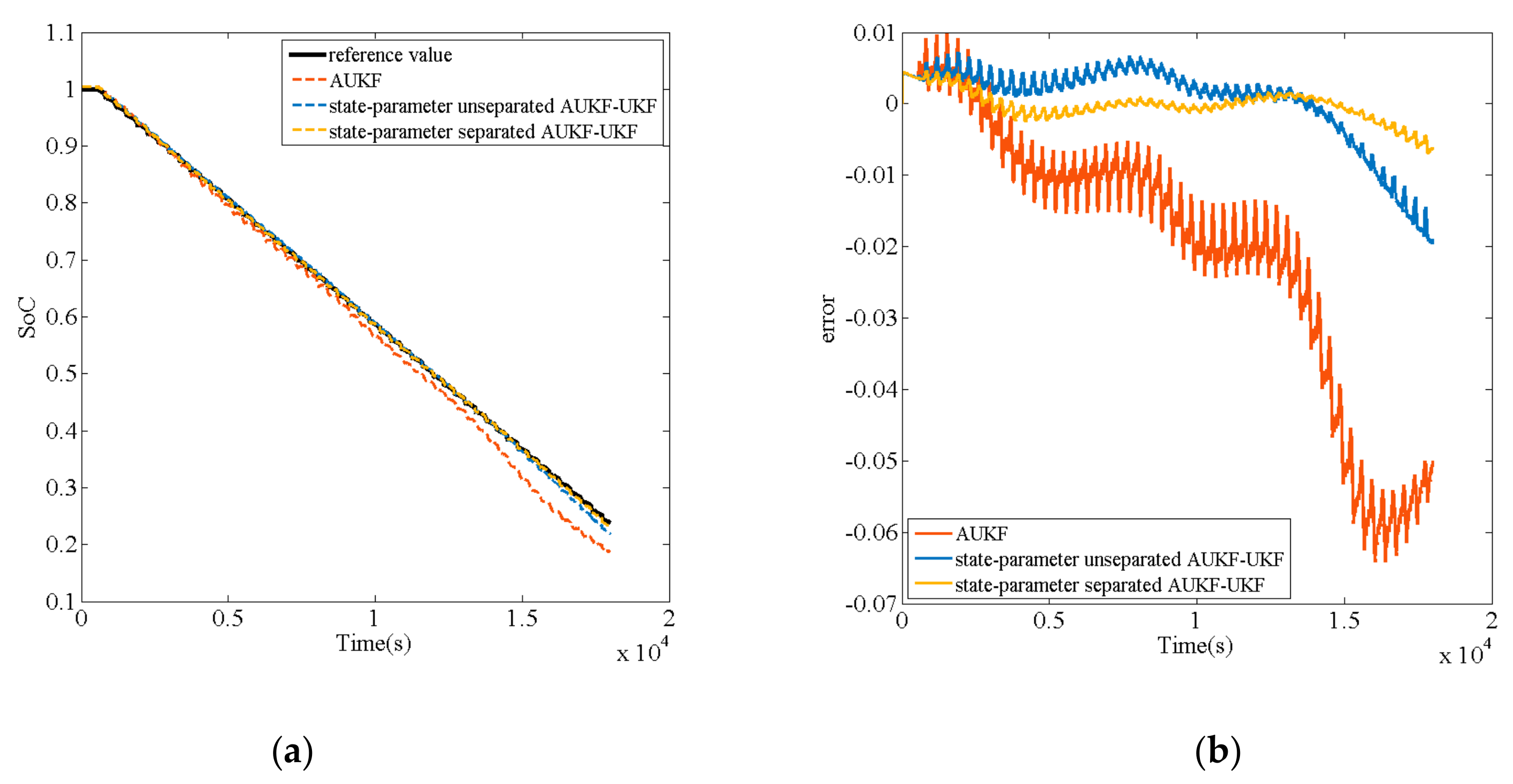
5.3.2. Comparison of Convergence Performance
6. Conclusions
Author Contributions
Funding
Acknowledgments
Conflicts of Interest
References
- Huangfu, Y.; Xu, J.; Zhao, D.; Liu, Y.; Gao, F. A novel battery state of charge estimation method based on a super-twisting sliding mode observer. Energies 2018, 11, 1211. [Google Scholar] [CrossRef]
- Hannan, M.A.; Xu, J.; Lipu, M.S.H.; Hussian, A.; Mohamed, A. A review of lithium-ion battery state of charge estimation and management system in electric vehicle applications: Challenges and recommendations. Renew. Sustain. Energy Energies 2017, 78, 834–854. [Google Scholar] [CrossRef]
- Patrick, J.; Michael, V.; Daniel, R.; David, V.; Werner, J.; Jürgen, G. An electrochemical impedance spectroscopy study on a lithium sulfur pouch cell. Adv. Radio Sci. 2016, 14, 55–62. [Google Scholar]
- Stroe, D.I.; Knap, V.; Swierczynski, M.; Stanciu, T.; Schaltz, E.; Teodorescu, R. An electrochemical impedance spectroscopy study on a lithium sulfur pouch cell. ECS Trans. 2016, 72, 13–22. [Google Scholar] [CrossRef]
- Xing, Y.; He, W.; Pecht, M.; Tsui, K.L. State of charge estimation of lithium-ion batteries using the open-circuit voltage at various ambient temperatures. Appl. Energy 2014, 113, 106–115. [Google Scholar] [CrossRef]
- Chiang, Y.H.; Sean, W.Y.; Ke, J.C. Online estimation of internal resistance and open-circuit voltage of lithium-ion batteries in electric vehicles. J. Power Sour. 2011, 196, 3921–3932. [Google Scholar] [CrossRef]
- Guo, L.; Hu, C.; Li, G. The SOC estimation of battery based on the method of improved ampere-hour and Kalman filter. In Proceedings of the 10th Conference on Industrial Electronics and Applications, Auckland, New Zealand, 15–17 June 2015; pp. 1458–1460. [Google Scholar]
- Chen, Z.; Qiu, S.; Masrur, M.A.; Murphey, Y.L. Battery state of charge estimation based on a combined model of extended Kalman filter and neural networks. In Proceedings of the International Joint Conference on Neural Networks, San Jose, CA, USA, 31 July–5 August 2011; pp. 2156–2163. [Google Scholar]
- Antón, J.C.A.; Nieto, P.G.; de Cos Juez, F.J.; Lasheras, F.S.; Vega, M.G.; Gutiérrez, M.R. Battery state-of-charge estimator using the SVM technique. Appl. Math. Modell. 2013, 37, 6244–6253. [Google Scholar] [CrossRef]
- Malkhandi, S. Fuzzy logic-based learning system and estimation of state-of-charge of lead-acid battery. Eng. Appl. Artif. Intell. 2006, 19, 479–485. [Google Scholar] [CrossRef]
- Zhang, C.; Allafi, W.; Dinh, Q.; Ascencio, P.; Marco, J. Online estimation of battery equivalent circuit model parameters and state of charge using decoupled least squares technique. Energy 2018, 142, 678–688. [Google Scholar] [CrossRef]
- Plett, G.L. Extended Kalman filtering for battery management systems of LiPBbased HEV battery packs. Section 1. Background. J. Power Sour. 2004, 134, 252–261. [Google Scholar] [CrossRef]
- Plett, G.L. Extended Kalman filtering for battery management systems of LiPBbased HEV battery packs. Section 2. Modeling and identification. J. Power Sour. 2004, 134, 262–276. [Google Scholar] [CrossRef]
- Plett, G.L. Extended Kalman filtering for battery management systems of LiPBbased HEV battery packs. Section 3. State and parameter estimation. J. Power Sour. 2004, 134, 277–292. [Google Scholar] [CrossRef]
- Plett, G.L. Sigma-point Kalman filtering for battery management systems of LiPBbased HEV battery packs: Section 2: Simultaneous state and parameter estimation. J. Power Sour. 2006, 161, 1369–1384. [Google Scholar] [CrossRef]
- Andre, D.; Appel, C.; Soczka-Guth, T.; Sauer, T.U. Advanced mathematical methods of SOC and SOH estimation for lithium-ion batteries. J. Power Sour. 2013, 224, 20–27. [Google Scholar] [CrossRef]
- Guo, F.; Hu, G.; Xiang, S.; Zhou, P.; Hong, R.; Xiong, N. A multi-scale parameter adaptive method for state of charge and parameter estimation of lithium-ion batteries using dual Kalman filters. Energy 2019, 178, 79–88. [Google Scholar] [CrossRef]
- Zhang, X.; Wang, Y.; Yang, D.; Chen, Z. An on-line estimation of battery pack parameters and state-of-charge using dual filters based on pack model. Energy 2016, 115, 219–229. [Google Scholar] [CrossRef]
- Wang, Q.; Kang, J.; Tan, Z.; Luo, M. An online method to simultaneously identify the parameters and estimate states for lithium ion batteries. Electrochim. Acta 2018, 289, 376–388. [Google Scholar] [CrossRef]
- Chen, Z.; Yang, L.; Zhao, X.; Wang, Y.; He, Z. Online state of charge estimation of Li-ion battery based on an improved unscented Kalman filter approach. Appl. Math. Modell. 2019, 70, 532–544. [Google Scholar] [CrossRef]
- Wang, Q.; Wang, J.; Zhao, P.; Kang, J.; Yan, F.; Du, C. Correlation between the model accuracy and model-based SOC estimation. Electrochim. Acta 2017, 228, 146–159. [Google Scholar] [CrossRef]
- Johnson, V.H. Battery performance models in ADVISOR. J. Power Sour. 2002, 110, 321–329. [Google Scholar] [CrossRef]
- Simon, H. KALMAN Filtering and Neural Networks; John Wiley & Sons: New York, NY, USA, 2001; pp. 1–10. [Google Scholar]
- Zhang, F.; Liu, J.; Fang, J. Battery State Estimation Using Unscented Kalman Filter. In Proceedings of the IEEE International Conference on Robotics and Automation, Kobe, Japan, 12–17 May 2009. [Google Scholar]
- Peng, S.M.; Chen, C.; Shi, H.B. State of charge estimation of battery energy storage systems based on adaptive unscented kalman filter with a noise statistics estimator. IEEE Access 2017, 5, 13202–13212. [Google Scholar] [CrossRef]
- USCAR.Manuals: Electrical Vehicle Battery Test Procedures Manual. Available online: http://www.uscar.org/guest/publications (accessed on 30 August 2017).
- Xiong, R.; Yu, Q.; Wang, Y.; Lin, C. A novel method to obtain the open circuit voltage for the state of charge of lithium ion batteries in electric vehicles by using H infinity filter. Appl. Energy 2017, 207, 346–353. [Google Scholar] [CrossRef]


| Parameters | Value |
|---|---|
| Nominal Capacity | 40 Ah |
| Nominal Voltage | 3.7 V |
| Max Charge Voltage | 4.2 V |
| Min Discharge Voltage | 3.2 V |
| Parameters | K0 | K1 | K2 | K3 | K4 | K5 | K6 |
|---|---|---|---|---|---|---|---|
| Value | 3.43 | 0.3725 | 5.862 | −32.58 | 68.02 | –60.73 | 19.8 |
| Identification Area | Long Discharge Recovery | Pulse Discharge | ||||||
| Parameters | τ1 (s) | τ2 (s) | τ1 (s) | τ2 (s) | R1 (Ω) | R2 (Ω) | R0 (Ω) | |
| SoC= | 0.902 | 1613 | 79.94 | 16.13 | 1.001 | 0.0010 | 0.000278 | 0.0017 |
| 0.834 | 2695 | 150.22 | 14.13 | 0.741 | 0.0011 | 0.000227 | 0.0017 | |
| 0.705 | 2045 | 274.57 | 12.70 | 0.640 | 0.0011 | 0.000218 | 0.0017 | |
| 0.607 | 2149 | 126.33 | 15.40 | 0.831 | 0.0011 | 0.000239 | 0.0017 | |
| 0.508 | 2838 | 193.57 | 14.18 | 0.765 | 0.0008 | 0.000211 | 0.0017 | |
| 0.410 | 2973 | 268.96 | 12.20 | 0.582 | 0.0007 | 0.000205 | 0.0017 | |
| 0.312 | 2458 | 327.44 | 12.70 | 0.589 | 0.0008 | 0.000249 | 0.0018 | |
| 0.213 | 2670 | 332.12 | 11.51 | 0.468 | 0.0008 | 0.000346 | 0.0018 | |
| 0.115 | 4390 | 414.77 | 11.84 | 0442 | 0.0012 | 0.000613 | 0.0018 | |
| Algorithms | Items | Errormax | RMSE |
|---|---|---|---|
| AUKF | SoC estimation | 0.0631 | 0.0122 |
| uL prediction | 0.1865 V | 0.0066 V | |
| Open loop model output | 0.1904 V | 0.0097 V | |
| state-parameter unseparated AUKF-UKF | SoC estimation | 0.0404 | 0.00104 |
| uL prediction | 0.0403V | 0.00049 V | |
| Open loop model output | 0.0405 V | 0.0056 V | |
| state-parameter separated AUKF-UKF | SoC estimation | 0.0187 | 0.00056 |
| uL prediction | 0.0474 V | 0.00092 V | |
| Open loop model output | 0.0461 V | 0.0034 V |
| Algorithms | Items | Errormax | RMSE |
|---|---|---|---|
| AUKF | SoC estimation | 0.0642 | 0.0279 |
| uL prediction | 0.0109 V | 0.0031 V | |
| Open loop model output | 0.0323 V | 0.0129 V | |
| State-parameter unseparated AUKF-UKF | SoC estimation | 0.0195 | 0.00059 |
| uL prediction | 0.0109 V | 0.0008 V | |
| Open loop model output | 0.0191 V | 0.00041 V | |
| State-parameter separated AUKF-UKF | SoC estimation | 0.0069 | 0.00021 |
| uL prediction | 0.0115 V | 0.00092 V | |
| Open loop model output | 0.0131 V | 0.00022 V |
| Initial Value | 0.9 | 0.8 | 0.7 | 0.6 | 0.5 |
|---|---|---|---|---|---|
| Convergence time (s) | 390 | 600 | 1023 | 1310 | 2065 |
© 2019 by the authors. Licensee MDPI, Basel, Switzerland. This article is an open access article distributed under the terms and conditions of the Creative Commons Attribution (CC BY) license (http://creativecommons.org/licenses/by/4.0/).
Share and Cite
Yu, C.-X.; Xie, Y.-M.; Sang, Z.-Y.; Yang, S.-Y.; Huang, R. State-Of-Charge Estimation for Lithium-Ion Battery Using Improved DUKF Based on State-Parameter Separation. Energies 2019, 12, 4036. https://doi.org/10.3390/en12214036
Yu C-X, Xie Y-M, Sang Z-Y, Yang S-Y, Huang R. State-Of-Charge Estimation for Lithium-Ion Battery Using Improved DUKF Based on State-Parameter Separation. Energies. 2019; 12(21):4036. https://doi.org/10.3390/en12214036
Chicago/Turabian StyleYu, Chuan-Xiang, Yan-Min Xie, Zhao-Yu Sang, Shi-Ya Yang, and Rui Huang. 2019. "State-Of-Charge Estimation for Lithium-Ion Battery Using Improved DUKF Based on State-Parameter Separation" Energies 12, no. 21: 4036. https://doi.org/10.3390/en12214036
APA StyleYu, C.-X., Xie, Y.-M., Sang, Z.-Y., Yang, S.-Y., & Huang, R. (2019). State-Of-Charge Estimation for Lithium-Ion Battery Using Improved DUKF Based on State-Parameter Separation. Energies, 12(21), 4036. https://doi.org/10.3390/en12214036