Article

A Mixed Uncertainty Power Flow Algorithm-Based Centralized Photovoltaic (PV) Cluster

1
School of Electrical Engineering, Chongqing University, Chongqing 400044, China
2
State Key Laboratory of Power Transmission Equipment & System Security and New Technology, Chongqing University, Chongqing 400044, China
*
Author to whom correspondence should be addressed.
Energies 2019, 12(20), 4008; https://doi.org/10.3390/en12204008
Submission received: 18 September 2019 / Revised: 17 October 2019 / Accepted: 17 October 2019 / Published: 22 October 2019
(This article belongs to the Section F: Electrical Engineering)

Abstract

:
With the large-scale centralized PV clusters connected to grid, the grid power flow has certain randomness. Considering the fluctuation of PV output, an improved Krawczyk-Moore algorithm in a mixed coordinate system is proposed to solve the uncertain power flow problem. Firstly, aiming at the special structure of a centralized PV cluster with only load node and no generator node, this paper proposes a power flow calculation in the mixed power flow coordinate, and then the Krawczyk-Moore operator is used to combine interval and affine arithmetic to overcome the shortcoming of over-conservative interval algorithm. Finally, the voltage operating condition under different volatility and different partial shading conditions is studied through the simulation of a practical example, and the out-of-limit voltage problem inside the centralized PV cluster is analyzed. Meanwhile, the effectiveness of the proposed algorithm is verified.

1. Introduction

With the increasingly severe global energy crisis, developing renewable energy has become the consensus of the whole human society. The development of renewable energy is also an inevitable trend in future power systems [1]. As a widely utilized renewable energy, solar energy has been developing rapidly in the world, especially in China in recent years. According to national energy-related data, by the end of 2018, China had added 44 GW of PV installations, with a total installed capacity of 174 GW, including 124 GW of centralized PV clusters [2].
Power flow analysis is one of the most fundamental and heavily used tools in power engineering, such as reactive power optimization, state estimation, and fault diagnosis [3]. It allows power system analysts to determine the steady state or operating conditions of a power system for a specified set of values, such as load and generation levels. Power flow calculation is the basis of power flow analysis. On the one hand, power flow calculation can provide the basis for the selection of electrical equipment and the optimization of power supply schemes for power system planning; on the other hand, it can provide the analysis of static security and adjust operation mode for the power system, as well as provide the initial data for fault calculation and stability calculation of the power system. However, due to the fluctuation of PV cells, the original deterministic power flow calculation model is no longer applicable. As centralized PV clusters undertake more and more power transmission tasks in the power grid, its stable operation is crucial to the stability of the entire power grid. In order to ensure the safe, stable, and reliable operation of power systems, it is particularly important to study the uncertain power flow algorithm of centralized PV clusters [4,5].
At present, there are three main calculation methods for uncertain power flow: (1) The fuzzy mathematical method [6,7]; (2) the probability power flow method, which mainly includes the analytical method [8,9], the approximation method [10] and the simulation method [11]; and (3) interval analysis [12,13,14]. When the first and second kinds of methods are adopted, the probability density function or membership function of uncertain parameters needs to be known; due to the randomness of data, these functions are difficult to be determined in practice and usually rely on presetting. Considering the above limitations, the third type, the interval analysis method, is considered to be an effective method to solve the problem of uncertain power flow because it only needs to determine the range of variables, which is simple to model. In addition, interval analysis can avoid the interference of human factors, which has been paid close attention by researchers [15]. Based on the existing research results, the calculation methods of interval power flow are mainly divided into the affine optimization method, the direct optimization method, and the iterative method [16]. In [17], an affine-based interval power flow analysis method was proposed. By solving a power flow equation and two linear programming problems, the upper and lower bounds of the power flow solutions that restrain interval extension were obtained. In [18], Taylor expansion of intervals was carried out according to affine ideas, and interval power flow equations in the Cartesian coordinate system were expanded into three deterministic power flow equations for solution, which avoids interval iteration process. However, as with [18], the complexity of the calculation is increased by Taylor expansion. In [19], an interval optimization framework was proposed. Upper and lower bounds of power flow solutions were obtained respectively by solving two deterministic optimization problems. Reference [20] proposed a new optimization scenario method, which regarded the uncertainty of the interval as bounded variables and solved these unknown variables using the two methods of minimum programming model and maximum programming model, which determined the range of interval power flow problem. In [21], the Ybus Gaussian iterative interval power flow equation in complex affine form was established considering the uncertainty of the operation of distributed power supply. The iterative process was simplified and the accuracy and efficiency of interval power flow calculation were improved by using the method of noise element merging. In [22], the Krawczyk-Moore operator was used to combine interval and affine to achieve the requirement of overcoming interval conservatism.
However, in [17,18], Taylor expansion was adopted, which undoubtedly increased the amount of calculation and made the calculation process too tedious. When using the affine optimization method, the objective function and constraint conditions need to be constructed. Whereas, due to the large number of nodes in the PV cluster, the curse of dimensionality may occur due to too many constraints, eventually leading to the failure of the algorithm. In [19,20], the interval power flow solution problem can be converted into the maximum and minimum solution problem. However, a large amount of computational resources is consumed in the optimization process, and it is difficult to find the global optimal solution. In [21], when the iterative method is used, the accuracy may be insufficient due to the structure of the algorithm itself. Moreover, this method is only applicable to small-scale systems and DC power flow models, and is not applicable to the research object in this paper. In [22], the initial interval affects the convergence of iteration. When the output of PV cells within the cluster fluctuate greatly, non-convergence may occur. In [6,7,8,9,10,11,12,13,14,15,16,17,18,19,20,21,22], only the uncertainty of power was studied, and there was no specific research object. In [23,24,25], the centralized PV cluster was taken as the research object, but only to study their external characteristics, namely the fluctuation of output, without considering the huge internal network structure, which ignores the operation fluctuation of each PV generation unit within the cluster.
In order to solve the above problem, this paper proposes an improved algorithm based on the iterative method for the special structure of centralized PV clusters. The algorithm utilizes interval and affine arithmetic to process the Jacobi matrix elements in the two coordinate systems, and uses the K-operator to conduct iteration, respectively. At the end of each iteration, it is transformed into polar coordinate form for intersection processing, and then determines whether the iteration stop condition is satisfied or not, and finally gets the more ‘constricted’ interval result. The advantages of this algorithm are as follows: (1) The convergence performance of the Krawczyk-Moore operator is improved by processing the initial interval of iteration; (2) the mixed power flow avoids the waste of computing resources and saves computing time; (3) the application of affine arithmetic is expanded to overcome the shortcoming of too conservative interval results.
The rest of the paper is organized as follows: Section 2 presents the internal structure and modeling of centralized PV clusters. In Section 3, the principle of uncertain power flow algorithm is introduced. Section 4 introduces the modeling and iterative steps of mixed uncertain power flow. The voltage operating condition under different volatility and different partial shading conditions is analyzed in Section 5. The main conclusions and contributions of the paper are drawn in the last section.

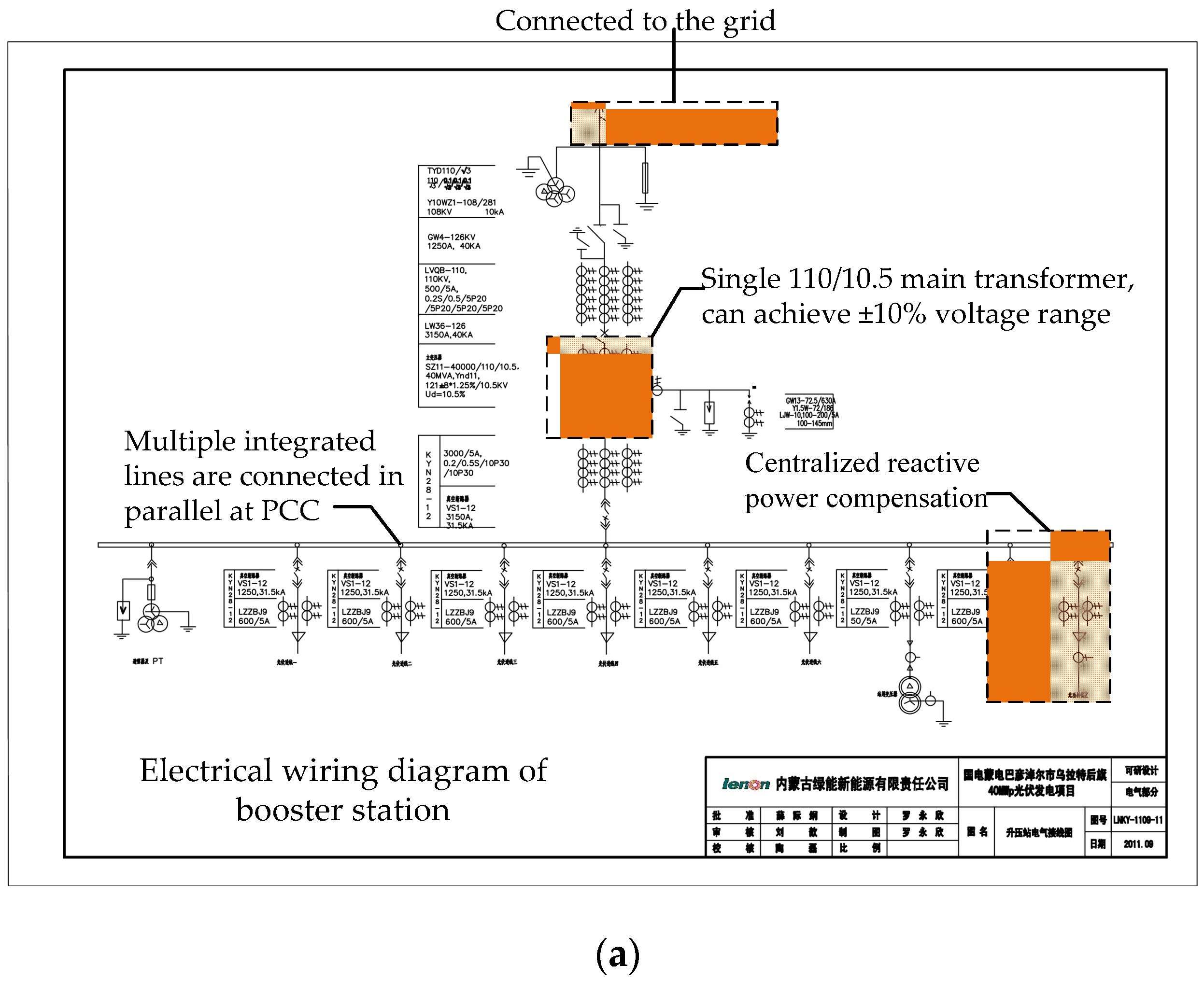
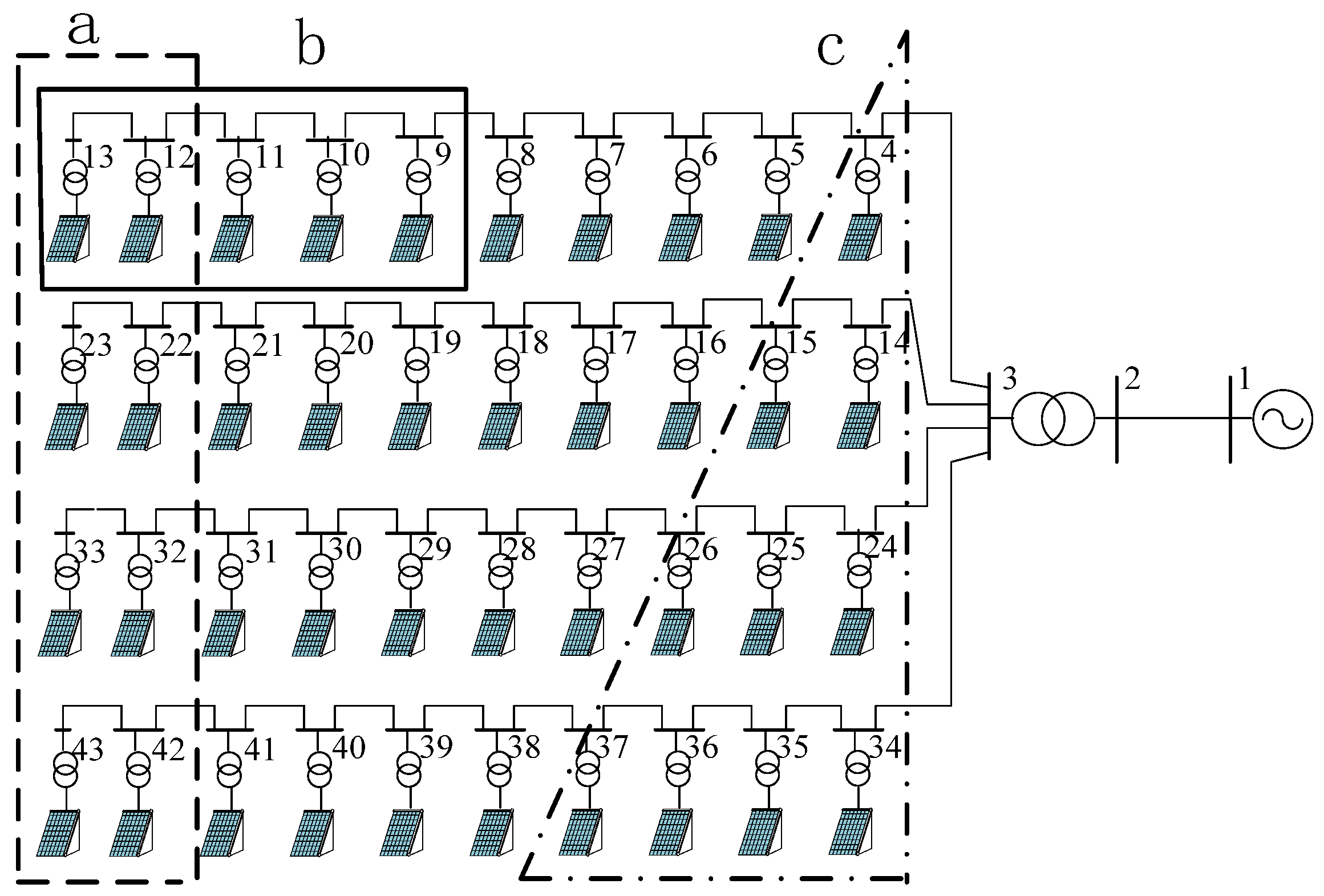
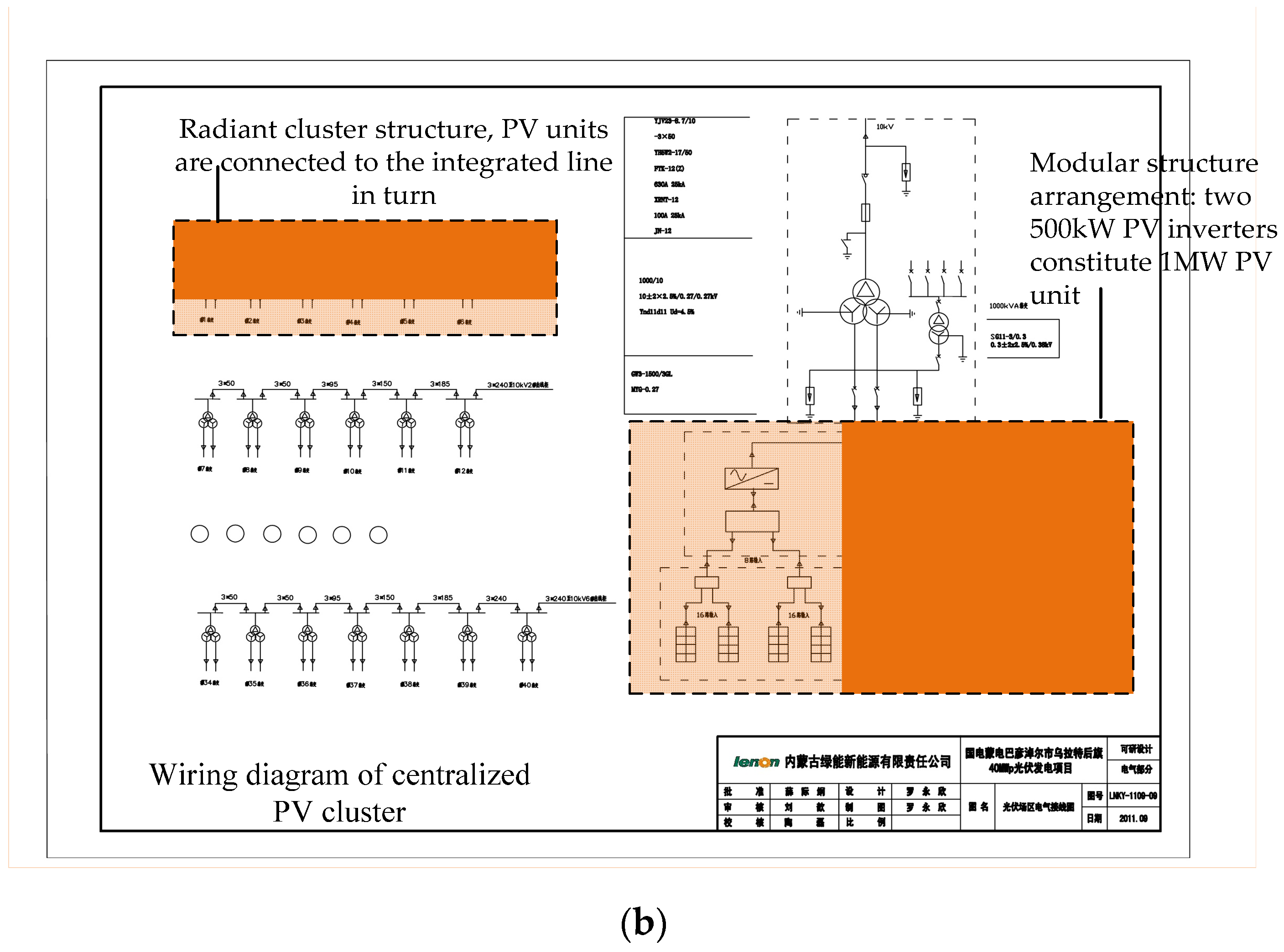
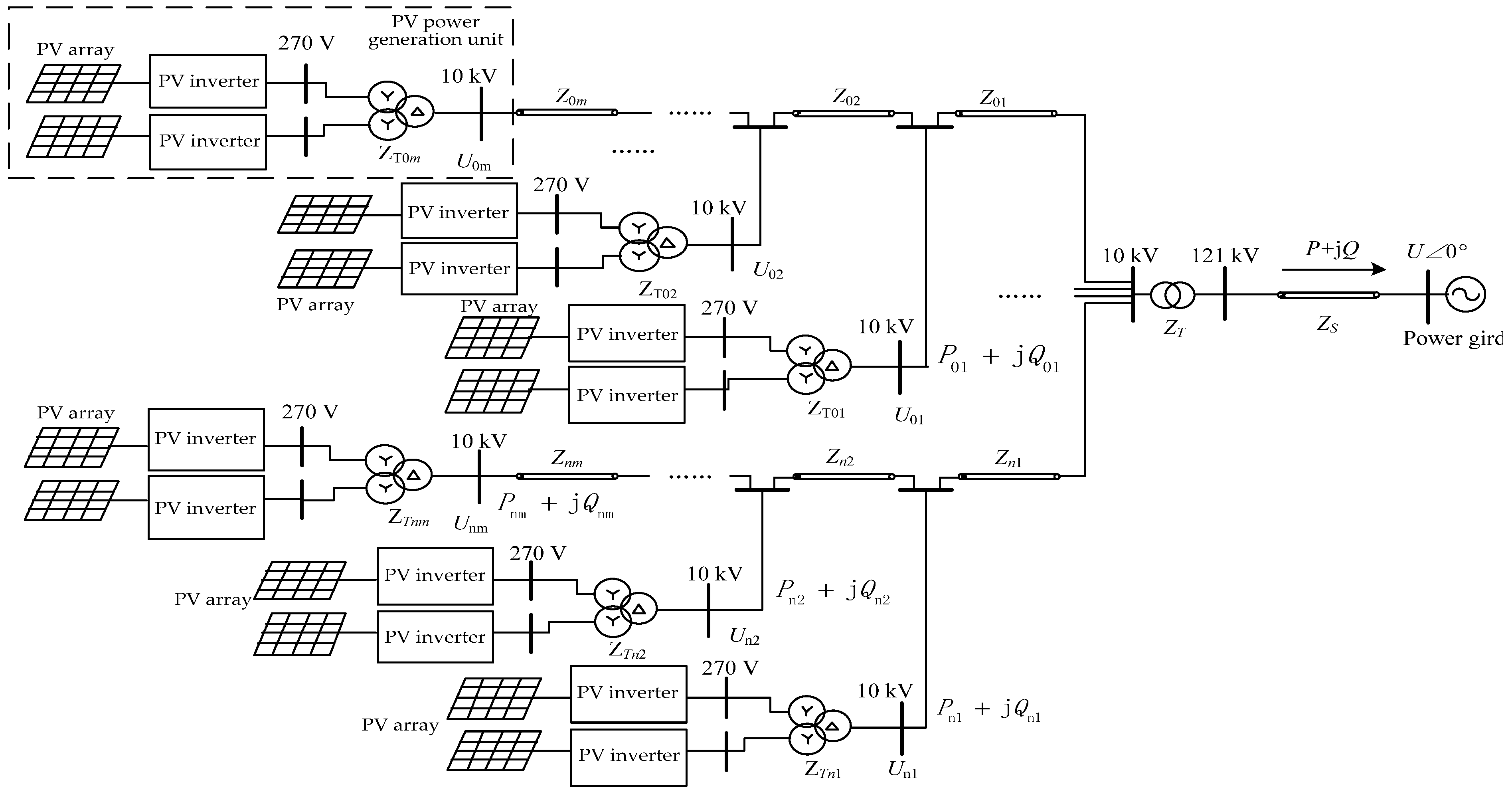
2. Centralized PV Clusters

2.1. Description of Centralized PV Clusters

Most of the centralized PV clusters are built away from the load in remote areas, which are weak grid structures over a long transmission distance and the voltage stability is poor.
As is shown in Figure 1, a PV unit consists of a PV array, two inverters, and a 0.27 kV/10kV transformer. A large number of PV units are series-connected in multiple branches, which are integrated in parallel, forming a radiant cluster structure. Then, the main transformer boosts the voltage to 110 kV, and the power is transmitted to the power grid through the high-voltage ac transmission line. It can be seen that there is a huge structure inside the cluster, which contains a large number of PV units, with a large amount of node information. However, in the previous analysis of the transmission network, the centralized PV cluster was considered a node, while the power flow analysis and research within the centralized PV cluster were ignored.

2.2. Modeling of PV Power Generation Units

PV power generation units transform the solar energy into electricity, of which the output is affected by light intensity, the exposed area of the cell, conversion efficiency, and other factors [26,27]. Its maximum output power is expressed as below:
P = η A S [ 1 0.005 ( T L 25 ) ]
where η is the conversion efficiency; A is the area of PV panels; S is the light intensity; TL is the temperature of PV panel.
For a particular centralized PV cluster, the area of the PV power generation unit is determined. Without considering factors such as PV unit aging, PV conversion efficiency is a fixed constant, usually 17%. Generally, the ambient temperature is used to calculate the temperature of PV cells, as shown in Equation (2):
T L T a + C S
where Ta is the ambient temperature and C is the influence factor of light intensity on temperature, which is 0.03.
According to the above, the output power of each PV power generation unit is:
P = η A S [ 1 0.005 ( T a + C S 25 ) ]
It can be seen from Equation (3) that the output of the PV unit is mainly affected by light intensity and has volatility. The inverter is assumed to work normally and outputs active power. All PV units are regarded as load nodes, power flow analysis is carried out within the centralized PV cluster, and the operation status of each node and its influence on the whole internal system are studied.

2.3. Impedance Modeling and Voltage Out-of-Limit Analysis of Centralized PV Clusters

The impedance of the centralized PV cluster is shown in Figure 2. In order to facilitate the study, the admittance of the split transformer in the PV power generation unit is neglected. The impedance in the cluster mainly includes the split-transformer impedance in the PV power generation unit, the integrated line impedance between adjacent PV power generation units, and the main transformer impedance. Grid impedance mainly includes ac transmission line impedance. Where Z T n m is the transformer impedance of the PV power generation unit; Z n m is the integrated line impedance between adjacent PV power generation units; Z T is the main transformer impedance; Z S is the transmission line impedance.
The voltage of the grid connection point of the centralized PV cluster is closely related to the voltage of the PV power generation unit within the cluster and the parameters of the integrated line [28]. Figure 2 shows that the structure of each line within the cluster is approximately the same. Taking the first line as an example, the node voltage is analyzed as shown in Equation (4):
U 0 i = U 0 ( i 1 ) + ( k = i m P 0 k P loss ) R 0 i + ( k = i m Q 0 k Q loss ) X 0 i U 0 ( i 1 )
where U 0 i and U 0 ( i 1 ) are the outlet voltage of the ith and i-1th PV power generation unit; R 0 i and X 0 i are the resistance and reactance of the transmission line between the ith PV power generation unit and the i-1th PV power generation unit; P 0 k , Q 0 k represent the active and reactive power output of the kth PV power generation unit; P loss and Q loss represent the active and reactive power lost on the integrated line before the ith PV power generation unit.
It can be seen from Equation (4) that node voltage keeps rising with the increase of node label. For one of the lines, the terminal PV power generation unit has the highest voltage. The resistance value of the internal integrated lines of the centralized PV cluster is much higher than the reactance value. With the increasing installed capacity of centralized PV clusters, fluctuations in the output of PV power generation units will cause large fluctuations in the voltage of internal node and grid connection point, and even cause serious out-of-limit voltage problems, affecting the safe and stable operation of the entire power system.

3. Interval Analysis

3.1. Interval Arithmetic

The method of interval analysis is used to solve the problem of uncertain power flow in the centralized PV cluster, so that all solutions are included in the interval. Use interval form to express the range of uncertain quantity, for given real numbers x ¯ and x ¯ R , If x ¯ x ¯ is satisfied, then the closed bounded set x ~ = [ x ¯ , x ¯ ] is called bounded interval [29]. The basic algorithm of defining interval is shown in Equation (5):
{ x ~ + y ~ = [ x ¯ + y ¯ , x ¯ + y ¯ ] x ~ y ~ = [ x ¯ y ¯ , x ¯ y ¯ ] x ~ × y ~ = [ min ( x ¯ y ¯ , x ¯ y ¯ , x ¯ y ¯ , x ¯ y ¯ ) , max ( x ¯ y ¯ , x ¯ y ¯ , x ¯ y ¯ , x ¯ y ¯ ) ] x ~ / y ~ = [ x ¯ , x ¯ ] [ 1 / y ¯ , 1 / y ¯ ]    0 y ~
Other algorithms related to intervals can be referred to in [29], which will not be listed in this paper. It can be seen from the above that interval operations are conservative. For example, an interval number x ~ = [ 1 , 3 ] , then x ~ x ~ 0 .

3.2. Affine Arithmetic

As can be seen from the above example, the interval operation ignores the correlation between two interval numbers, the result of interval operation is often larger than the actual range, which is the conservatism of interval operation. To improve the conservative interval operation, affine operation is proposed in [28], which takes the correlation between interval variables into account. A more ‘constricted’ interval solution is thus obtained. The basic affine form is shown in Equation (6).
x ^ = x 0 + x 1 ε 1 + x 2 ε 2 + x n ε n = x 0 + i = 1 n x i ε i
where x ^ represents uncertain variable; x 0 is the mid-range; ε i is the noise item, which is within the interval [ 1 , 1 ] ; x i is the coefficient of the ith noise term, representing the influence of corresponding noise term on uncertain variables. The basic operation of affine arithmetic can be referred to in [30].
Interval arithmetic and affine arithmetic are interchangeable. Given an interval number x ~ = [ x ¯ , x ¯ ] , it is converted into the second-order affine form by Equation (7). Given an affine number x 0 + i = 1 n x i ε i , it is converted to interval form by Equation (8).
{ x ^ = x 0 + x 1 ε 1 x 0 = x ¯ + x ¯ 2 x 1 = x ¯ x ¯ 2
{ x ¯ = x 0 i = 1 n | x i | x ¯ = x 0 + i = 1 n | x i |
Similarly, for the example in Section 2.1, the interval form is converted to affine form x ^ x ^ = 0 . If the same noise term appears in the two affine numbers, it means that they are related. The more noise terms that exist in the form, the closer the relation of they are. This is how affine operation overcomes the interval conservatism and make the calculation result more accurate.

3.3. Krawczy-Moore Interval Operator

The Newton iteration method is considered to be an effective method for solving nonlinear equations, x = y f ( y ) ( f ( x ) ) 1 . Moore builds on this by introducing interval variables for interval mapping; the uncertain nonlinear equations can be solved, and the iteration form is as follows: x ~ = m ( x ~ ) f ( m ( x ~ ) ) ( F m ( x ~ ) ) 1 , where m ( x ~ ) is the midpoint of the interval.
However, in the iterative process above, the interval inverse matrix is complex. Based on the fixed-point theorem, Krawczyk improved it with avoiding the inverse process of interval matrix, and effectively simplified the iterative process. In this paper, the Krawczyk-Moore interval operator is used to solve the uncertain power flow problem, and the iterative algorithm is shown in Equation (9):
{ x ~ i + 1 = x ~ i K ( x ~ i ) K ( x ~ i ) = y i Y i f ( y i ) + ( I Y i F ( x ~ i ) ) ( x ~ i y i ) y i = m ( x ~ i ) Y i = ( m ( F ( x ~ i ) ) ) 1
where F ( x ~ i ) is the interval Jacobi matrix and Y i is the inverse matrix of the midpoint value of the F ( x ~ i ) .

4. Interval Analysis

4.1. Mixed Uncertain Power Flow Model for Centralized PV Clusters

For centralized PV clusters, there are only load nodes, without generator nodes in the whole network. When the polar coordinate is used to represent the power flow equation or the rectangular coordinate is used to represent the power flow equation, the number of equations is the same. Therefore, power flow calculation will be carried out at the same time in two coordinates. The deterministic power flow equation of the centralized PV cluster in polar coordinates and rectangular coordinates is shown in Equations (10) and (11):
{ Δ P = P i U i j = 1 n U j ( G i j cos θ i j + B i j sin θ i j ) = 0 Δ Q = Q i U i j = 1 n U j ( G i j sin θ i j B i j cos θ i j ) = 0
{ Δ P = P i j = 1 n [ e i ( G i j e j B i j f j ) + f i ( G i j f j + B i j e j ) ] = 0 Δ Q = Q i j = 1 n [ f ( G i j e j B i j f j ) + e i ( G i j f j + B i j e j ) ] = 0
where P i is the active power output of the ith PV power generation unit, which can be obtained according to Equation (3), and Q i is 0 in the case of unity power factor operation. For the convenience of expression, the above power flow equation is expressed as f ( x ) = 0 .
The fluctuation of the PV power generation unit output leads to the failure of traditional deterministic power flow algorithm. Therefore, combining Equations (9)–(11), the uncertain power flow model of the centralized PV cluster can be obtained as shown in Equation (12).
{ x ~ 1 = [ θ ~ U ~ ] = [ [ θ ¯ , θ ¯ ] [ U ¯ , U ¯ ] ] x ~ 2 = [ f ~ e ~ ] = [ [ f ¯ , f ¯ ] [ e ¯ , e ¯ ] ] F ( x ~ ) = [ H ~ J ~ N ~ L ~ ] y i = m ( x ~ i ) f ( y i ) = f ( m ( x ~ i ) ) Y = ( m ( F ( x ~ ) ) ) 1
In the whole iterative calculation process, affine operation exists in Y i F ( x ~ i ) , ( I Y i F ( x ~ i ) ) ( x ~ i y i ) and Y i f ( y i ) ( I Y i F ( x ~ i ) ) ( x ~ i y i ) . Finally, affine results are uniformly transformed into interval results.

4.2. The Processing of Jacobi Matrix Elements

Section 3.1 introduces the mixed uncertain power flow model of the centralized PV cluster. Compared with the traditional deterministic power flow model, the difference lies in the interval form or affine form when calculating each element of the Jacobi matrix.
{ H ~ i j = Δ P ~ i θ ~ j = U ~ i U ~ j ( G i j sin θ ~ i j B i j cos θ ~ i j ) H ~ i i = Δ P ~ i θ ~ i = j = 1 , i j n U ~ i U ~ j ( G i j sin θ ~ i j B i j cos θ ~ i j )
{ H ~ ij = Δ P ~ i f ~ j = B i j e ~ i + G i j f ~ i H ~ ii = Δ P ~ i f ~ i = 2 G ii f ~ i + j = 1 , j i n ( G i j f ~ j + B i j e j )
In this paper, considering the strong correlation between trigonometric functions sin θ ~ i j and cos θ ~ i j in Equation (13), as well as the strong correlation between e ~ i and f ~ i in rectangular coordinates in Equation (14). The Jacobi element form of a mixed power flow calculation is shown below.
{ H ~ i j = U ~ i U ~ j G i j 2 + B i j 2 sin ( θ ~ i j + δ i j ) H ~ i i = j = 1 , i j n U ~ i U ~ j G i j 2 + B i j 2 sin ( θ ~ i j + δ i j ) δ i j = arctan ( B ij / G ij )
{ H ^ i j = B i j e ^ i + G i j f ^ i H ^ i i = 2 G i i f ^ i + j = 1 , i j n ( G i j f ^ j + B i j e ^ j )
By using different methods to the Jacobi elements in the two coordinate forms, the range can be reduced effectively and different results can be obtained. The rest of the elements are handled the same way.

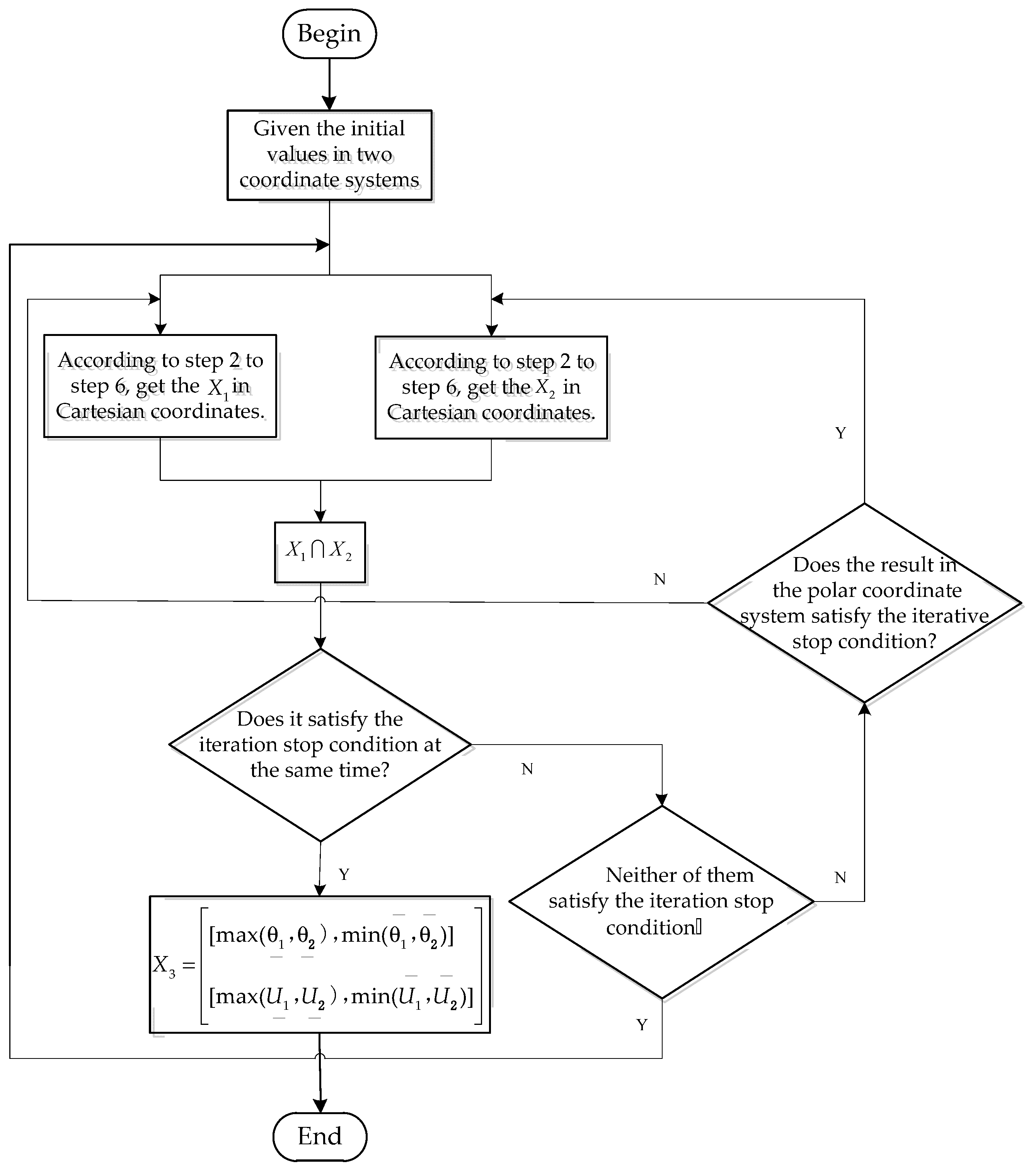
4.3. Calculation Steps of Mixed Uncertain Power Flow

Step 1: The interval expansion based on the deterministic power flow solution of the upper and lower limits of power fluctuation can ensure the relatively small range of the initial iteration interval and effectively reduce the number of iterations. Set the initial value of the independent variable as:
x ~ 0 = [ a ~ b ~ ] = [ [ a ¯ , a ¯ ] [ b ¯ , b ] ] ,
where a ~ and b ~ represent θ ~ and U ~ in the polar coordinate system, f ~ and e ~ in the rectangular coordinate system, respectively.
Step 2: The mixed form Jacobi matrix F ( x ~ i ) is calculated according to Equations (15) and (16).
Step 3: Extract the mean value of the interval form and the real term of the affine form of each Jacobi element, and find the inverse matrix to get the real matrix Y i .
Step 4: Convert the interval form to affine form, and compute ( I Y i F ( x ~ i ) ) ( x ~ i y i ) and Y i f ( y i ) in affine form.
Step 5: Calculate K ( x ~ i ) in affine form and convert it to interval form.
Step 6: x ~ i + 1 = x ~ i K ( x ~ i ) .
Step 7: The results of the two coordinate systems are mixed by using the method in this paper. The specific mixing process is shown in Figure 3.

5. Simulation Analysis

5.1. Simulation Parameter Setting

In order to verify the effectiveness of the proposed algorithm in this paper, a centralized PV cluster system in China is taken as an example in Figure 4. The K-operator algorithm combined with affine (hereinafter referred to as affine algorithm) proposed in [22], the algorithm in this paper, and the Monte Carlo method are used for comparative analysis. Node 1 is set as the slack bus, and the remaining nodes are load nodes. Set the reference capacity as 10 MW and the reference voltage as 10 KV. The power fluctuation range of load nodes is set as ±10%. Convergence accuracy is ω = 10 5 .
The total installed capacity of the centralized PV cluster is 40 MW, which is composed of four integrated lines in parallel. Each integrated line is composed of 10 PV power generation units in series. Each PV power generation unit has a capacity of 1 MW (including two inverters with a capacity of 500 kW) and is connected to the integrated line through split transformer with a capacity of 1.5 MVA. The integrated line between adjacent PV power generation units is 1 km long and connected by cable of model YJV 23 - 8.7 / 10 , 3 × 150   mm 2 . The main transformer capacity is 60 MW. The transmission line is 100 km long and adopts the overhead line of LGJ185. Data parameters are shown in Table 1 and Table 2. The PV power generation unit output is set to 0.7 MW according to Equation (3), in the case of unity power factor operation. Reactive power compensation device is added at the PCC (point of common coupling).

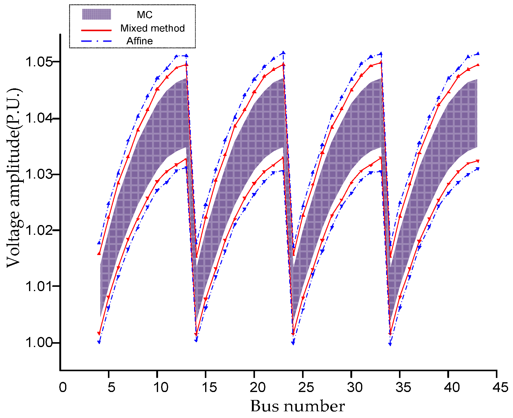
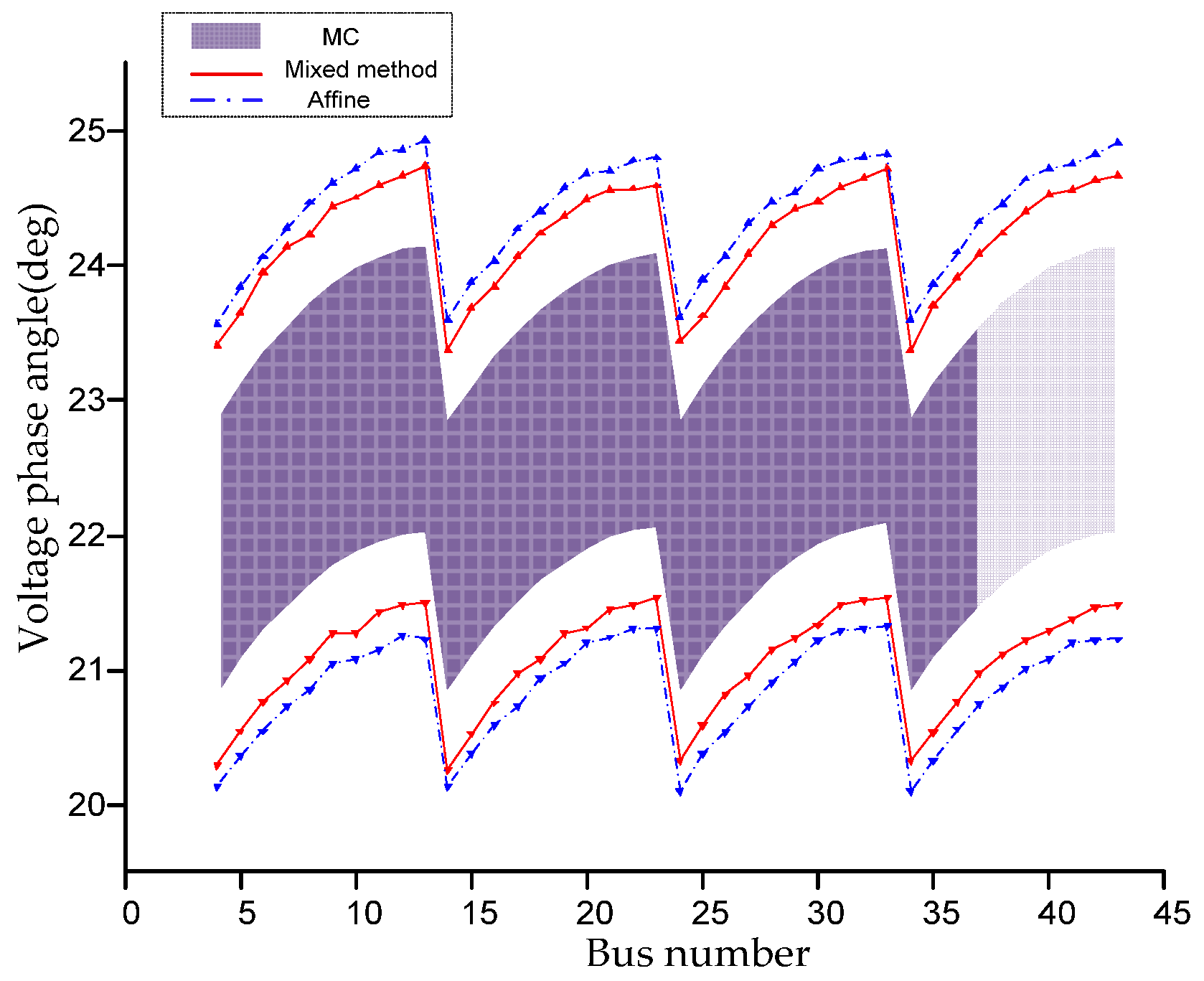
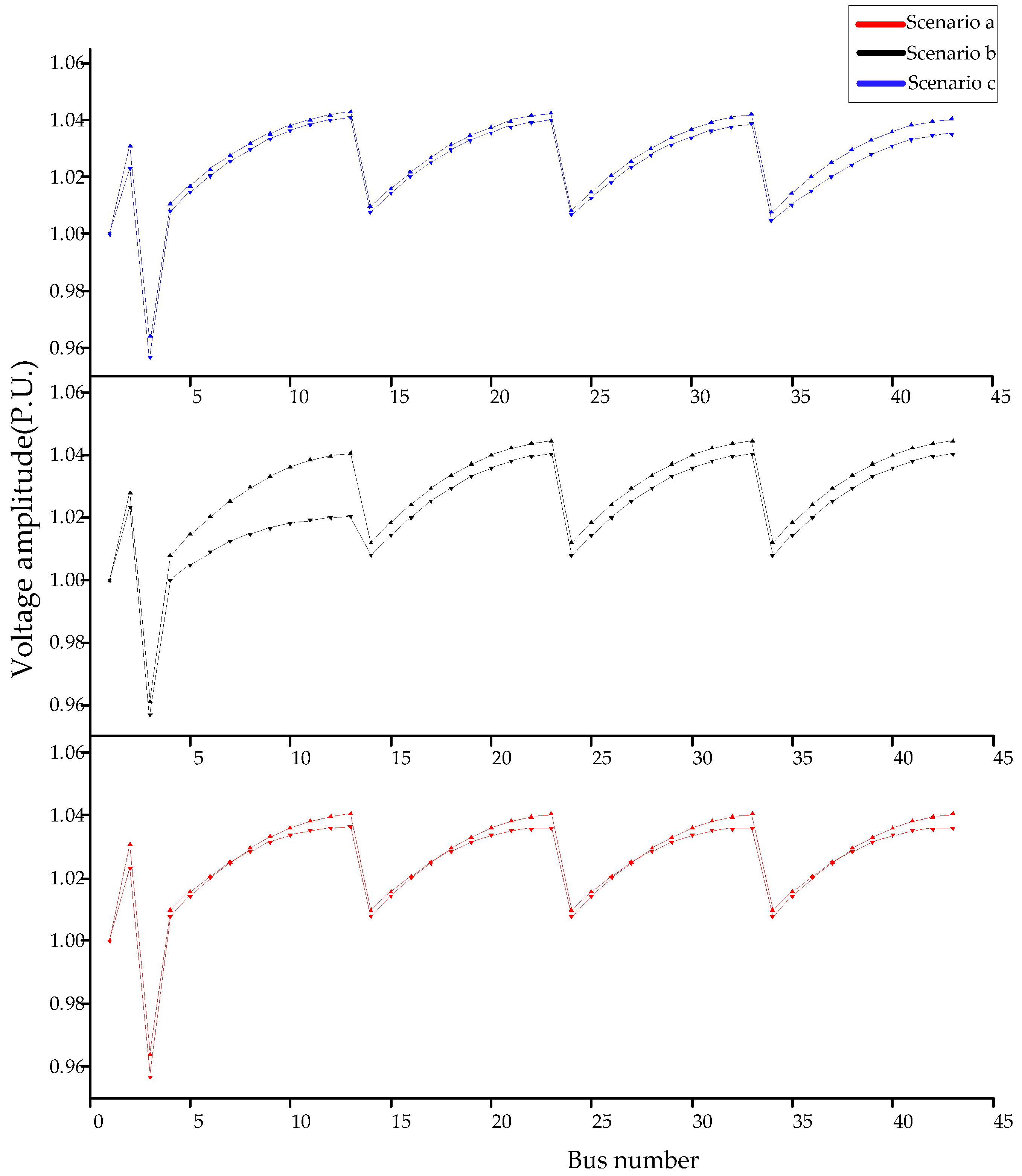
5.2. Comparison and Analysis of Simulation Results for Centralized PV Clusters

The Monte Carlo method obtains multiple sets of solutions through a large number of repeated sampling calculations, and then expresses them in interval form as the exact solution of uncertain power flow (in fact, the range of interval obtained by this method is smaller than the real). In the simulation test in this paper, the sampling random numbers of the Monte Carlo method obey uniform distribution within the power fluctuation range, and the results of 4000 deterministic power flow calculations are taken as interval results. Affine algorithm proposed in literature [22], the method presented in this paper and Monte Carlo method were used for simulation calculation. The simulation results of the voltage amplitude and phase angle of nodes 2 and 3 are shown in Table 3 and Table 4. The voltage amplitude and phase Angle of PV power generation unit node are shown in Figure 5 and Figure 6.
As can be seen from the chart above, the results of node voltage amplitude and phase angle obtained by the algorithm in this paper include all solutions of the Monte Carlo method, which proves the completeness of the algorithm proposed in this paper. Moreover, the interval range is more ‘constricted’ than the results obtained by the method in reference [22], which effectively reduces the interval range. This is due to the expansion of the application of affine arithmetic in the calculation of the K-operator algorithm and the full consideration of the correlation of interval elements. With the mixed power flow algorithm, the calculated results complement each other. In previous studies, these factors were not fully considered, resulting in relatively conservative interval results. In this paper, the upper bound and lower bound maximum error rates η are used to evaluate the relative error of the results, and the results are shown in Table 5.
η = max ( | X ¯ i x ¯ i x ¯ i | , | X i ¯ x i ¯ x i ¯ | ) × 100 % , i ( 2 , 43 )
where X ¯ i and X i ¯ are the upper and lower bounds of simulation results obtained with the proposed algorithm and the affine algorithm, and x ¯ i and x i ¯ are the upper and lower bounds of simulation results obtained by the Monte Carlo method.
As can be seen from Table 5, for the voltage relative error rate, the phase relative angle error rate obtained by the proposed algorithm is relatively large. In the calculation of the mixed power flow, the upper and lower limits of the real part and the imaginary part of voltage are generally not reached at the same time. Therefore, the reduction of the range of interval is not obvious in the mixing process, during which the Cartesian coordinates are converted into polar coordinates.
For the voltage amplitude interval results in Figure 5, it can be seen that as the number of nodes of each integrated line PV power generation unit increases, the voltage amplitude becomes larger, and the PV power generation unit outlet at the end of the line faces the risk of out-of-limit voltage, which also verifies the correctness of Equation (4). According to Table 3, the internal node 3 of the centralized PV cluster is also facing the risk of out-of-limit voltage. Considering the special structure of the centralized photovoltaic cluster with only load nodes, mixed power flow calculation is adopted in this paper, which is carried out in two coordinate systems at the same time. No more computing resources were consumed during the whole computing process, and the consumption time was 2.8 s, which is almost the same as that of the improved previous K-operator algorithm (2.7 s), and higher calculation accuracy is achieved. This is nearly 50 times faster than the Monte Carlo method (138.6 s).

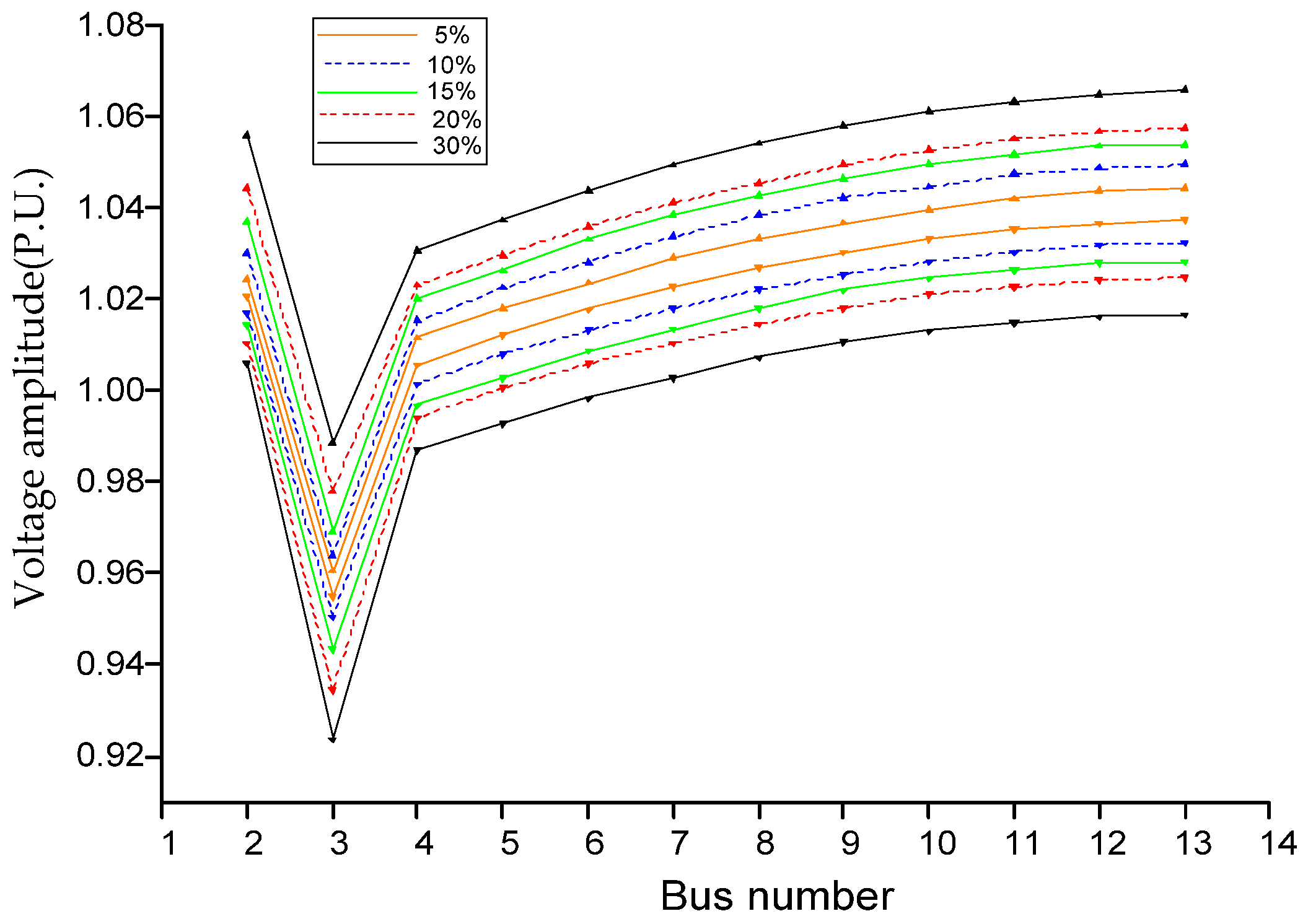
5.3. Voltage Operating Condition Under Different Volatility

Based on the system setup in Section 4.1, the voltage amplitude variation range of the centralized PV cluster with different volatility is studied.
Considering the internal structure of the centralized PV cluster, due to the similar operation conditions of each integrated line, only the nodes of the first branch are selected for analysis. As can be seen from Figure 7, the amplitude of node voltage variation becomes larger with the increase of output fluctuation of the PV power generation unit. In addition, the number of nodes with out-of-limit voltage also increases. When the power fluctuation range reaches 30%, most PV power generation units are faced with the problem of out-of-limit voltage. The voltage amplitude fluctuation range at PCC (node 3) is larger than the voltage amplitude fluctuation range at the outlet of the PV power generation unit, which is also faced with a serious out-of-limit voltage problem. With the increase of the power fluctuation range, the lower limit of voltage of node 2 is closer to the voltage of slack bus, reactive power is required to be absorbed from the grid to maintain the normal operation of the centralized PV cluster. Through the simulation analysis above, it can be seen that there is a serious risk of out-of-limit voltage within the centralized PV cluster, which may even lead to the interlocking disconnection of the PV power generation units and influence stability of the power grid. Therefore, it is necessary to strengthen the monitoring and regulation of PCC and terminal PV power generation units for more efficient and reliable power flow analysis, which can ensure the normal operation of each PV unit within the cluster and the safe grid-connected centralized PV clusters.

5.4. Voltage Operating Condition Under Different Partial Shading Conditions

As is shown in Figure 4, voltage distribution inside the cluster under different partial shading conditions is studied. In this paper, it is assumed that the lower limit of output fluctuation is 50% when the PV units are partially shaded. This part selects the following three partial shading conditions to research: (1) The PV unit at the end of each integrated line shows the same degree of partial shading; (2) in the first integrated line, partial shading occurs in some PV units; and (3) the PV units of each integrated line have different degrees of shading conditions.
As can be seen from Figure 8, the voltage distribution inside the centralized PV cluster is different under different partial shading conditions. For scenario a, the node voltage range of four integrated lines within the cluster is the same because of the same shading condition of each integrated line. For scenario b, the voltage amplitude of this integrated line varies greatly because partial shading only occurs in this integrated line. In this scenario, there are a large number of PV generation units with partial shading at the end of the integrated line. It can also be deduced from Equation (4) that, when the terminal PV generation unit occurs a violent power fluctuation, it will have a violent impact on all the voltage distributions of the integrated line. For scenario c, each integrated line has different degrees of shading, and the voltage range of each integrated line is therefore different. When partial shading occurs in the centralized PV cluster, the voltage at the PCC will decrease, resulting in the overall drop of the voltage in the station. In addition, by comparing the results under the three scenarios, it can be seen that: (1) The more PV generation unit with partial shading, the greater the voltage fluctuation of the integrated line; (2) compared with the PV generation unit at the start of the integrated line, when the PV generation unit at the terminal of the integrated line appears partial shading, the voltage fluctuation is larger. From the analysis above, it can be seen that when partial shading occurs, uneven voltage distribution will occur in the cluster, which may lead to out-of-limit voltage problems and even affect the stable operation of the whole system.

6. Conclusions

In order to ensure the safe and reliable operation of power systems, the power flow calculation of the centralized PV cluster was carried out, and an improved uncertain power flow algorithm of K-operator based on mixed power flow was proposed. The main conclusions are as follows:
(1) In this paper, internal network structure was considered and the power flow calculation was carried out inside the PV cluster. According to the results, a more ‘constricted’ interval, with the voltage error within 0.20–0.28% of the proposed method, was obtained. Interval expansion was effectively suppressed. For the calculation time, the proposed method takes less time (2.8 s) than the Monte Carlo method (138.6 s).
(2) According to the simulation results, when the power fluctuation occurs, the voltage amplitude of the whole cluster changes dramatically, and the PV unit at the end of the integrated line is faced with a serious out-of-limit voltage problem. It is concluded that no matter where the internal fault occurs, it will have a huge impact on the operation of the PV unit at the end. The study in this paper has some guiding significance for the field of reactive power optimization.

Author Contributions

Conceptualization, H.W. and L.Z.; Methodology, H.W.; Software, S.Z. and H.W.; Formal Analysis, Q.L.; Resources, L.Z.; Writing—Original Draft Preparation, H.W.; Writing—Review and Editing, Y.W.; Supervision, L.Z.; Project Administration, L.Z.

Funding

This research was funded by the National Natural Science Foundation of China, grant number 51707026, and the Graduate Research and Innovation Foundation of Chongqing, grant number CYS18007.

Conflicts of Interest

The authors declare no conflicts of interest.

References

  1. Liu, D.; Liu, M.; Xu, E. Comprehensive effectiveness assessment of renewable energy generation policy: A partial equilibrium analysis in China. Energy Policy 2018, 115, 330–341. [Google Scholar] [CrossRef]
  2. China Photovoltaic Industry Association. 2018. Available online: http://www.chinapv.org.cn (accessed on 31 March 2019).
  3. Niu, M.; Wan, C.; Xu, Z. A review on applications of heuristic optimization algorithms for optimal power flow in modern power systems. J. Mod. Power Syst. Clean Energy 2014, 2, 289–297. [Google Scholar] [CrossRef] [Green Version]
  4. Wang, Q.; Chang, P.; Bai, R. Mitigation Strategy for Duck Curve in High Photovoltaic Penetration Power System Using Concentrating Solar Power Station. Energies 2019, 12, 3521. [Google Scholar] [CrossRef]
  5. Xu, C.; Gu, W.; Gao, F. Improved affine arithmetic based optimisation model for interval power flow analysis. IET Gener. Transm. Distrib. 2016, 10, 3910–3918. [Google Scholar] [CrossRef]
  6. Albatsh, F.M.; Ahmad, S.; Mekhilef, S. Fuzzy-Logic-Based UPFC and Laboratory Prototype Validation for Dynamic Power Flow Control in Transmission Lines. IEEE Trans. Ind. Electron. 2017, 64, 9538–9548. [Google Scholar] [CrossRef]
  7. Zhao, Q.; Shao, S.; Lu, L. A New PV Array Fault Diagnosis Method Using Fuzzy C-Mean Clustering and Fuzzy. Energies 2018, 11, 238. [Google Scholar] [CrossRef]
  8. Williams, T.; Crawford, C. Probabilistic Load Flow Modeling Comparing Maximum Entropy and Gram-Charlier Probability Density Function Reconstructions. IEEE Trans. Power Syst. 2013, 28, 272–280. [Google Scholar] [CrossRef]
  9. Fan, M.; Vittal, V.; Heydt, G.T. Probabilistic Power Flow Studies for Transmission Systems with Photovoltaic Generation Using Cumulants. IEEE Trans. Power Syst. 2012, 27, 2251–2261. [Google Scholar] [CrossRef]
  10. Caramia, P.; Carpinelli, G.; Varilone, P. Point estimate schemes for probabilistic three-phase load flow. Electr. Power Syst. Res. 2010, 80, 168–175. [Google Scholar] [CrossRef]
  11. Ni, F.; Nguyen, P.H.; Cobben, J.F.G. Basis-Adaptive Sparse Polynomial Chaos Expansion for Probabilistic Power Flow. IEEE Trans. Power Syst. 2017, 32, 694–704. [Google Scholar] [CrossRef]
  12. Wang, Z.; Alvarado, F.L. Interval arithmetic in power flow analysis. IEEE Trans. Power Syst. 1992, 7, 1341–1349. [Google Scholar] [CrossRef]
  13. Das, B. Radial distribution system power flow using interval arithmetic. Int. J. Electr. Power Energy Syst. 2002, 24, 827–836. [Google Scholar] [CrossRef]
  14. Pereira, L.E.S.; Da, C.V.M.; Rosa, A.L.S. Interval arithmetic in current injection power flow analysis. Int J. Electr. Power Energy Syst. 2012, 43, 1106–1113. [Google Scholar] [CrossRef]
  15. Ding, T.; Bo, R.; Li, F. Interval Power Flow Analysis Using Linear Relaxation and Optimality-Based Bounds Tightening (OBBT) Methods. IEEE Trans. Power Syst. 2015, 30, 177–188. [Google Scholar] [CrossRef]
  16. Liao, X.; Liu, K.; Le, J. Review on Interval Power Flow Calculation Methods in Power System. Proc. CSEE 2019, 39, 447–459. (In Chinese) [Google Scholar]
  17. Vaccaro, A.; Canizares, C.A.; Villacci, D. An Affine Arithmetic-Based Methodology for Reliable Power Flow Analysis in the Presence of Data Uncertainty. IEEE Trans. Power Syst. 2010, 25, 624–632. [Google Scholar] [CrossRef]
  18. Liao, X.; Liu, K.; Niu, H. An interval Taylor-based method for transient stability assessment of power systems with uncertainties. Int. J. Electr. Power Energy Syst. 2018, 98, 108–117. [Google Scholar] [CrossRef]
  19. Vaccaro, A.; Canizares, C.A.; Bhattacharya, K.A. Range Arithmetic-Based Optimization Model for Power Flow Analysis under Interval Uncertainty. IEEE Trans. Power Syst. 2013, 28, 1179–1186. [Google Scholar] [CrossRef]
  20. Zhang, C.; Chen, H.; Shi, K. An Interval Power Flow Analysis through Optimizing-Scenarios Method. IEEE Trans. Smart Grid 2017, 9, 5217–5226. [Google Scholar] [CrossRef]
  21. Wang, S.; Shao, Z. Interval power-flow algorithm based on complex affine Ybus-Gaussian iteration considering uncertainty of DG operation. Electr. Power Autom. Equip. 2017, 37, 38–44. (In Chinese) [Google Scholar]
  22. Ding, T.; Cui, H.; Gu, W. An uncertainty power flow algorithm based on interval and affine arithmetic. Autom. Electr. Power Syst. 2012, 36, 51–55. (In Chinese) [Google Scholar]
  23. Shah, R.; Mithulananthan, N.; Bansal, R.C. Power system voltage stability as affected by large-scale PV penetration. In Proceedings of the IEEE International Conference on Electrical Engineering and Informatics, Bandung, Indonesia, 17–19 July 2011. [Google Scholar]
  24. Pandey, A.; Jereminov, M.; Wagner, M.R. Robust Power Flow and Three-Phase Power Flow Analyses. IEEE Trans. Power Syst. 2019, 34, 616–626. [Google Scholar] [CrossRef]
  25. Wang, Y.; Wu, C.; Liao, H. Study on impacts of large-scale photovoltaic power station on power grid voltage profile. In Proceedings of the IEEE International Conference on Electric Utility Deregulation & Restructuring & Power Technologies, Nanjing, China, 6–9 April 2008. [Google Scholar]
  26. Daniela, F.; Paola, S.; Franco, F. Electroluminescence Test to Investigate the Humidity Effect on Solar Cells Operation. Energies 2018, 11, 2659. [Google Scholar] [Green Version]
  27. Alonso, G.G.; Michael, B.; Fernando, J.V. Shading Ratio Impact on Photovoltaic Modules and Correlation with Shading Patterns. Energies 2018, 11, 852. [Google Scholar] [Green Version]
  28. Nur, H.Z. Lightning Surge Analysis on a Large Scale Grid-Connected Solar Photovoltaic System. Energies 2017, 10, 2149. [Google Scholar] [Green Version]
  29. Alefeld, G.; Mayer, G. Interval analysis: Theory and applications. J. Comput. Appl. Math. 2000, 121, 421–464. [Google Scholar] [CrossRef]
  30. Figueiredo, L.D.; Stolfi, J. Affine arithmetic: Concepts and applications. Numer. Algorithms 2004, 37, 47–158. [Google Scholar] [CrossRef]
Figure 1. Take the centralized PV cluster in Bayannur city of Inner Mongolia province as an example to describe. (a) Electrical wiring diagram of boost station; (b) Wiring diagram of centralized PV clusters. Abbreviations: PV, photovoltaic; PCC, point of common coupling.
Energies 12 04008 g001aEnergies 12 04008 g001b
Figure 2. Line impedance of the centralized PV cluster.
Energies 12 04008 g002
Figure 3. Calculation process of the mixed power flow.
Energies 12 04008 g003
Figure 4. Diagram of the centralized PV cluster simulation system.
Energies 12 04008 g004
Figure 5. The voltage amplitude intervals of the PV power generation unit.
Energies 12 04008 g005
Figure 6. The voltage phase angle intervals of the PV power generation unit.
Energies 12 04008 g006
Figure 7. The voltage phase angle intervals under different volatility.
Energies 12 04008 g007
Figure 8. The voltage amplitude intervals under different partial shading conditions.
Energies 12 04008 g008
Table 1. The parameter of the line.
Type R ( Ω / km ) X ( Ω / km ) b ( Ω / km )
YJV23-8.7/100.1280.0113-
LGJ1850.170.4022.78 × 10−6
Table 2. The parameter of the transformer.
Type P 0 / kw P 0 / kw U d %
Split transformer1.15510.34.5%
Main transformer29.44148.810.5%
Table 3. Voltage amplitude intervals.
Node NumberMCMixed MethodAffine
2[1.0195, 1.0281][1.0171, 1.0302][1.0156, 1.0326]
3[0.9530, 0.9615][0.9506, 0.9638][0.9494, 0.9659]
Table 4. Voltage angle intervals.
Node NumberMCMixed MethodAffine
2[18.25, 20.11][17.71, 20.65][17.50, 20.89]
3[20.52, 22.50][19.95, 23.02][19.74, 23.24]
Table 5. Relative error rate.
TypeMixed MethodAffine
Voltage error rate0.20–0.28%0.38–0.46%
Phase angle error rate2.1–3.0%3.1–4.2%

