Article

A Stochastic-CVaR Optimization Model for CCHP Micro-Grid Operation with Consideration of Electricity Market, Wind Power Accommodation and Multiple Demand Response Programs

1
Department of Economic Management, North China Electric Power University, Baoding 071003, China
2
School of Economics and Management, North China Electric Power University, Beijing 102206, China
*
Author to whom correspondence should be addressed.
Energies 2019, 12(20), 3983; https://doi.org/10.3390/en12203983
Submission received: 22 August 2019 / Revised: 14 October 2019 / Accepted: 16 October 2019 / Published: 19 October 2019

Abstract

:
Combined cooling, heating and power (CCHP) micro-grids have the advantage of high energy efficiency, and can be integrated with renewable energies and demand response programs (DRPs). With the deepening of electricity market (EM) reforms, how to carry out operation optimization under EM circumstances will become a key problem for CCHP micro-grid development. This paper proposed a stochastic-CVaR (conditional value at risk) optimization model for CCHP micro-grid operation with consideration of EM participation, wind power accommodation and multiple DRPs. Specifically, based on the stochastic scenarios for EM clearing prices and wind power outputs uncertainties, the stochastic optimization method was applied to ensure the realization of operational cost minimization and wind power accommodation; the CVaR method was implemented to control the potential risk of operational cost increase. Moreover, by introducing multiple DRPs, the electrical, thermal and cooling loads can be transformed as flexible sources for CCHP micro-grid operation. Simulations were performed to show the following outcomes: (1) by applying the proposed stochastic-CVaR approach and considering multiple DRPs, CCHP micro-grid operation can reach better performance in terms of cost minimization, risk control and wind power accommodation etc.; (2) higher energy utilization efficiency can be achieved by coordinately optimizing EM power biddings; etc.

Graphical Abstract

1. Introduction

With the continuous development of the society and economy, energy and environmental issues have become increasingly prominent. Under the premise of satisfying people’s demand for multiple energy carriers, how to improve energy efficiency and achieve clean production have become a hot issue of current concern [1,2]. Due to the integration of distributed renewable generations, energy convertors, energy storages and multiple energy demands etc., the combined cooling, heating and power (CCHP) micro-grid provides an effective solution for this issue from a regional perspective [3,4,5].
The main question in the optimization of CCHP micro-grid operation is that what is optimum arrangement of energy components in each time period for providing multiple energy demands with minimum cost [6]. For CCHP micro-grid, the uncertainties such as distributed wind and/or photovoltaic (PV) power outputs etc., as well as the coupling of multi-energy flows are extremely challenging for its operation optimization [7]. Moreover, with the deepening of electricity market (EM) reforms in various countries around the world, the EMs have increasingly become the main platform for electrical energy trading [8]. Considering EM circumstances, the optimization of CCHP micro-grid operation needs to be further expanded, which brings extra difficulties. Specifically, (1) in addition to energy dispatch, offering/purchased power biddings in EM should also be coordinately optimized; (2) in addition to uncertainties such as renewable power outputs etc., it is also needed to take into account the stochastic interference brought by EM clearing prices. Hence, the optimization strategy for CCHP micro-grid operation under EM circumstances is studied in this paper.
At present, a number of researches have focused on the operation optimization problem for CCHP micro-grid/system. In [9,10], the performance of CCHP system operation following a hybrid electric-thermal load (FHL) was compared with the performance of CCHP system operation following the electric load (FEL) and the thermal load (FTL). It can be concluded in both [9] and [10] that the FHL strategy can make a better trade-off between cost and emission minimization compared with FEL and FTL strategies. References [11,12,13] and others have studied the optimal operation strategy of CCHP micro-grids based on deterministic programming methods such as linear programming [11], quadratic programming [12] and second-order cone programming [13], respectively. In these kinds of researches, uncertainties such as renewable power outputs etc. are ignored, and the scheduling results are difficult to ensure renewable energy accommodation. Soheyli et al. [14] introduced a multi-stage optimization method with consideration of the uncertainty of wind power output to economically dispatch a residential CCHP micro-grid. The simulation results show that the multi-stage optimization method is more conducive to wind power accommodation. Zhang et al. [15] proposed an online optimal operation model system for CCHP micro-grid based on model predictive control (MPC) method. In this model system, the uncertainties of both the renewable energy and loads were taken into account, and the reliable operation of CCHP micro-grid has been guaranteed through progressively solving this model system. Taking the advantage of the rapid regulation characteristics of gas turbines, Wang et al. [16] studied the wind power accommodation problem, and proposed a joint-dispatch scheme of energy and reserve for CCHP micro-grid. Case studies in [16] have validated that wind power accommodation can be significantly improved due to more reserve capabilities provided by implementing this scheme. In References [17,18,19,20,21,22], stochastic optimization (SO) frameworks were presented for the energy dispatches of various micro-grids. Shams et al. [17] proposed a two-stage SO model for the operation planning of micro-grids with multiple energy carriers, where uncertainties of renewable generations including the wind and PV are depicted by scenarios with respective probabilities. Simulations in [17] proved that the proposed two-stage SO model ensures the reliability and security of energy supply in multiple scenarios. Grover-Silva et al. [18] proposed a SO model for economic dispatch of flexible resources within a micro-grid environment, considering uncertainties of PV power outputs and electrical load. Additionally, the SO based dispatch models proposed in [19,20,21,22] have also been verified to provide optimal dispatch strategies and effectively reduce operational costs for CCHP micro-grids. In these SO models [17,18,19,20,21,22], uncertainties are described by stochastic scenarios. The dispatching principle is that when any scenario actually occurs, the operation can realize uncertainties accommodation through reasonable utilizations of controllable devices within various micro-grids. In [23,24,25,26], the optimization models for various micro-grids operations were constructed based on robust optimization (RO) method. Wang et al. [23] proposed a scheduling approach for micro-grid based on RO method. The simulation results of [23] verified the validity and effectiveness of the RO based approach for the micro-grid scheduling problem under uncertainties. Ji et al. [24] formulated the uncertainties of wind power and electrical load forecasting errors with the uncertainty set, and established a RO model for the optimal dispatch of micro-grid. Besides, the RO method was also applied in [25,26] for micro-grid operation to hedge against uncertainties from random renewable energy sources etc. In these RO models [23,24,25,26], uncertainties are estimated by uncertainty set. The dispatching principle is that when the worst scenario actually occurs, the dispatch of micro-grid can still maintain acceptable operational cost while accommodating uncertainties.
Moreover, demand response programs (DRPs), as new sources of system flexibility, have also been applied in the area of CCHP micro-grid operation. Saberi et al. [27] introduced the price-based DRP (electrical load shifting) concept into the multi-objective model for CCHP micro-grid operation. Simulated comparison revealed that the economic and environmental benefits of CCHP micro-grid can be further improved through the consideration of electrical load shifting. Varasteh et al. [28] introduced the incentive-based DRP (interruptible electrical load) into the bi-level optimization model for CCHP active micro-grid expansion and operation planning. A simulation test in [28] verified that the aggregated investment and operational costs can be significantly reduced by integrating interruptible electrical load. In the multi-objective operation optimization model proposed by Mohammadkhani et al. [29], the emission management of CCHP system was achieved via employing Time of Use (TOU) electricity tariff, reducible electrical load and Plug-in Hybrid Electric Vehicles. In addition to electrical load shifting, Vahid-Pakdel et al. [30] also implemented the thermal load shifting as thermal demand response program (TDRP) while constructing the SO model for energy hub (EH) operation. By introducing DRPs for multiple energy carriers, both the electrical and thermal loads can be transformed as flexible sources for reducing the operational cost of EH.
Recently, some studies also referred to the participations of distributed multi-energy systems (DMES) in EMs. Najafi et al. [31] considered both the energy dispatch and EM participation problems for an EH, and proposed an operation optimization model based on the conditional value at risk (CVaR) and SO methods, in which the uncertainties of day-ahead clearing prices and wind power outputs are formulated with multiple stochastic scenarios. Davatgaran et al. [32] introduced an electricity storage device into the structure of EH, and established an optimization model for multi-energy operation and power bidding in day-ahead EM based on SO method. In the study of Zhou et al. [33], a RO model was proposed for a multi-regional integrated energy system (MRIES) to coordinately optimize multi-energy operation and multi-stage power bidding. Hu (2017) et al. [34] established a CVaR based dispatch model for MRIES, in which the uncertainties of renewable power output were taken into account. Liu et al. [35] proposed an optimal bidding strategy in the day-ahead market of a micro-grid, where the uncertain renewable power output and day-ahead market price are modeled via scenarios based on forecast results. In the research of Najafi-Ghalelou et al. [36], RO method is provided for the scheduling of multi-energy hub system considering economic and environmental constraints in the presence of EM price uncertainty and electrical demand response programs (EDRP).
For the purpose of succinct demonstration, the above literature review is summarized in Table 1, in which some current research gaps are also presented.
According to the research gaps mentioned in Table 1, under the EM circumstances and integrated with multiple DRPs, the development of a reasonable optimization model for CCHP micro-grid operation is necessary and should at least achieve operational cost minimization, risk control against uncertainties and renewable power accommodation etc. Therefore, taking the day-ahead stage as illustration, this paper proposes a stochastic-CVaR optimization model for CCHP micro-grid operation with consideration of EM participation, wind power accommodation and multiple DRPs etc. The main contributions and novelties are as follows:
(1)
Through considering EM participation, it is further expanded in this paper the theory of CCHP operation optimization.
(2)
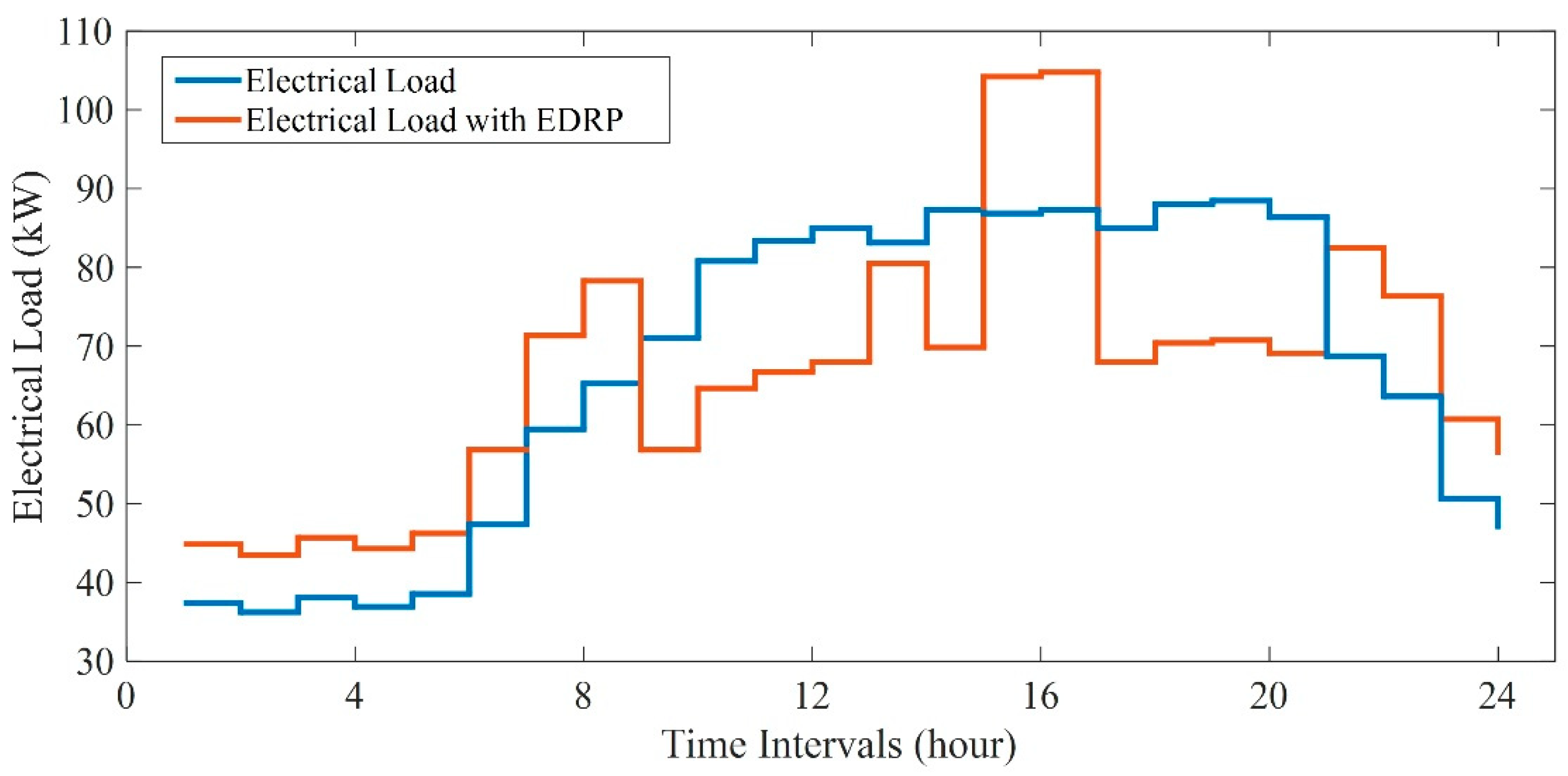
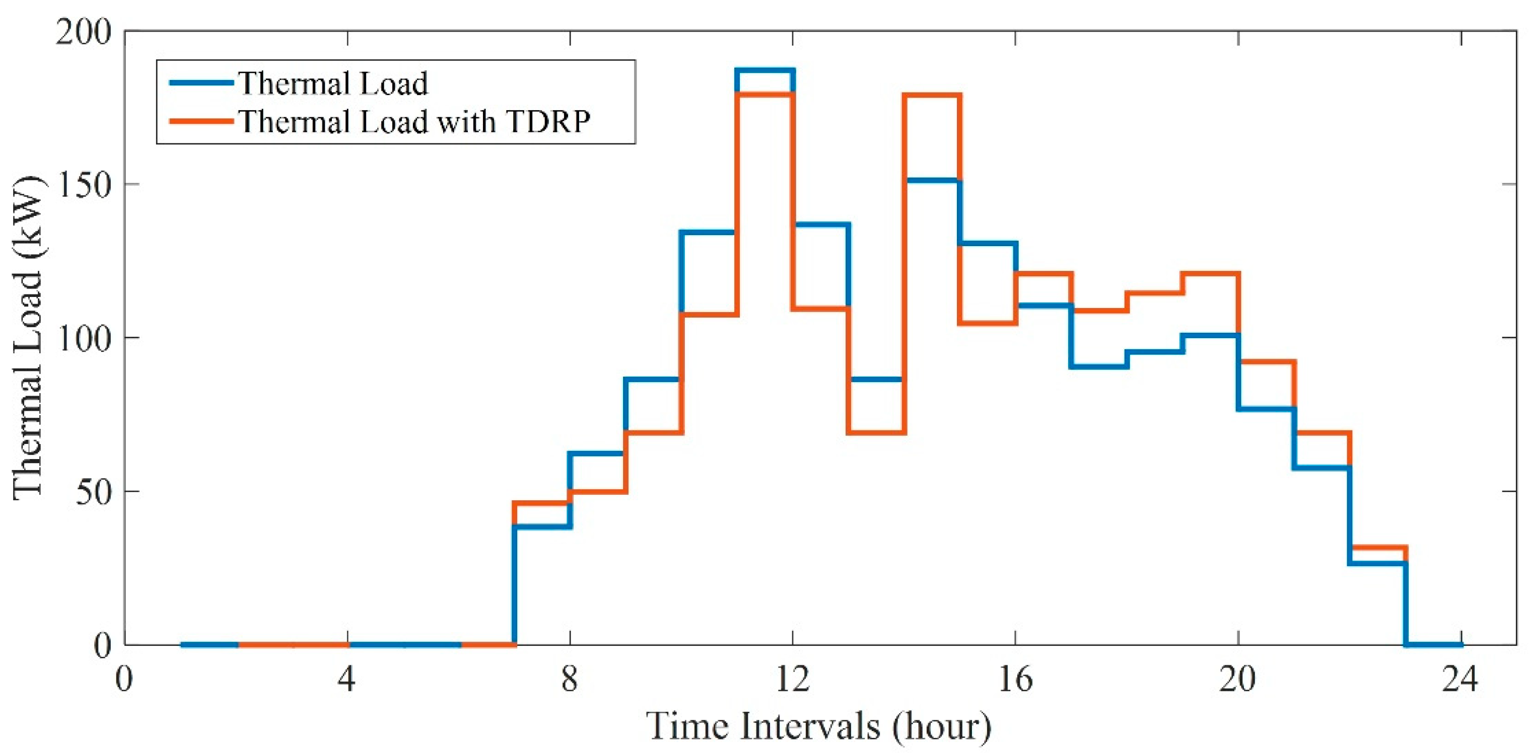
By introducing multiple DRPs (EDRP, TDRP and CDRP), the electrical, thermal and cooling loads can be transformed as flexible sources for better performance of CCHP micro-grid operation.
(3)
The CVaR theory for risk control is involved, which makes CCHP micro-grid reduce the potential risk of operational cost increase under the conditions of stochastic fluctuations of EM clearing prices etc.
(4)
By applying the SO method, uncertainties such as EM clearing prices and wind power outputs are depicted using stochastic scenarios. On the one hand, it is feasible to make the operation of CCHP micro-grid achieve operational cost minimization and wind power accommodation etc.; on the other hand, it is feasible to linearize the CVaR formulation, through which our proposed model is converted into a mixed integer linear programming (MILP), thus guaranteeing relatively low computational complexity and the existence of global optimum operation point.
The rest of this paper is organized as follows: Section 2 describes the structure and components modeling of CCHP micro-grid in detail. Section 3 is dedicated to formulate the optimization model for CCHP micro-grid operation. In Section 4 the simulation conditions and results have been explored. Finally, the conclusions are given in Section 5.

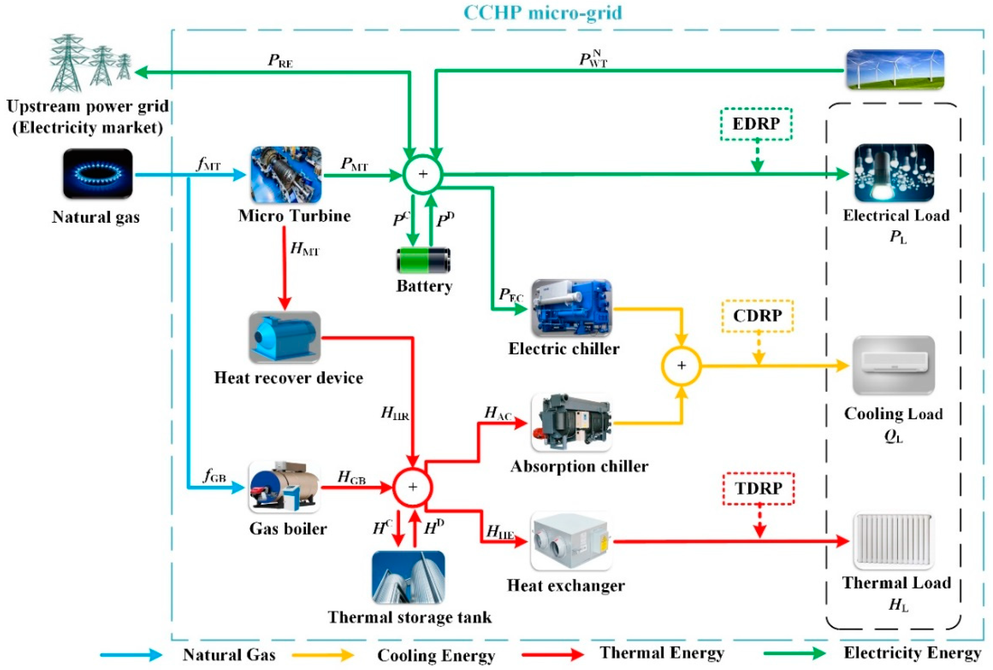
2. CCHP Micro-Gird Description and Modeling

Similar to [7], the typical structure of a CCHP micro-grid is as shown in Figure 1, which includes a micro turbine (MT), a wind turbine (WT), a gas boiler (GB), a heat recovery (HR) unit, a battery (BT), a thermal tank (TT), a heat exchanger (HE), an electrical chiller (EC) and an absorption chiller (AC), along with electrical, thermal and cooling loads. CCHP micro-gird’s electricity exchange with upstream power grid is achieved by participating in EMs. Besides, this work also takes multiple DRPs (e.g., EDRP, TDRP and CDRP) into consideration.
As mentioned in Section 1, considering the EM participation, CCHP micro-grid should coordinately optimize the multi-energy operation of its own components and power biddings with EMs. Obviously, due to the micro-grid characteristics, CCHP micro-grid can also meet its cooling, thermal and electrical loads by only dispatching its own components, which refers to as operating in islanded mode. In order to examine the effect of EM participation on CCHP micro-grid operation, comparative simulation studies between coordinately optimizing EM power biddings and islanded mode will be implemented in Section 4.3.

2.1. Micro Turbine

The amount of natural gas consumed by MT during time period t can be expressed as [34]:
f MT , t = P MT , t L H V ng η MT         t = 1 , , T
where, f MT , t indicates the amount of natural gas consumed by MT during time period t; P MT , t represents the power output of MT during time period t; coefficients L H V ng and η MT are the heat value of natural gas and the power efficiency of MT, respectively; T stands for the number of time periods for a delivery day.
Hence, the fuel cost of MT during time period t ( C MT , t ) can be calculated as follows:
C MT , t = C ng f MT , t         t = 1 , , T
where, C ng is the price of natural gas.
Correspondingly, the thermal power generated by MT during time period t ( H MT , t ) can be formulated as follows [33]:
H MT , t = ( 1 η MT η l ) η MT C O P h P MT , t         t = 1 , , T
where, η 1 means heat loss rate; C O P h is the coefficient of performance for MT.

2.2. Wind turbine

The relationship between WT’s (available) power output and wind speed can be approximated by [32,37,38]:
P WT , t = { 0 v t v ci ,   v t > v co k 1 v t + k 2 v ci < v t < v r P r v r v t v co         t = 1 , , T
where, P WT , t represents WT’s power output during time period t; v t represents the wind speed during time period t; P r means the rated power of WT; k 1 and k 2 are fitting parameters of the wind power-wind speed conversion curve; v ci is the cut-in wind speed; v r is the rated wind speed and v co is the cut-out wind speed.

2.3. Gas Boiler

The amount of natural gas consumed by GB during time period t can be expressed as:
f GB , t = H GB , t L H V ng C O P GB         t = 1 , , T
where, f GB , t indicates the amount of natural gas consumed by GB during time period t; H GB , t represents the thermal power output of GB during time period t; C O P GB is the coefficient of performance for GB.
Hence, the fuel cost of GB during time period t ( C GB , t ) can be calculated as follows:
C GB , t = C ng f GB , t         t = 1 , , T

2.4. Heat Recovery Unit

The relationship between the thermal power generated by MT and recovered by HR during time period t ( H HR , t ) can be formulated as follows [7]:
H HR , t = η HR H MT , t         t = 1 , , T
where, η H R is the recovery efficiency of HR.

2.5. Battery and Thermal Tank

For BT, the relationship between the residual energy and charging/discharging power during time period t can be formulated as follows [36]:
E t = E 0 + i = 1 t P i C η EC Δ t i = 1 t ( P i D / η ED ) Δ t         t = 1 , , T
E T = E 0
where, E 0 stands for the initial residual energy of BT; E t indicates the residual energy of BT at the end of time period t; Δ t is the duration of one time period; P t C and P t D represent charging and discharging powers of BT during time period t; η EC and η ED are charging and discharging efficiencies of BT.
Similarly, the relationship between the residual energy and thermal power stored/released by TT during time period t can be formulated as follows:
Ψ t = Ψ 0 + i = 1 t H i C η THC Δ t i = 1 t ( H i D / η THD ) Δ t         t = 1 , , T
Ψ T = Ψ 0
where, Ψ 0 stands for the initial residual energy of TT; Ψ t indicates the residual energy of TT at the end of time period t; H t C and H t D represent thermal powers stored and released by TT during time period t; η THC and η THD are stored and released efficiencies of TT.

2.6. Electrical and Absorption Chillers

The EC device consumes electrical energy to generate cooling energy. The relationship between electrical power input and cooling power output of EC can be formulated as follows [27]:
Q EC , t = P EC , t C O P EC         t = 1 , , T
where, Q EC , t and P EC , t stand for cooling power output and electrical power input of EC during time period t, respectively; C O P EC is the coefficient of performance for EC.
The AC device consumes thermal energy to generate cooling energy. The relationship between thermal power input and cooling power output of AC can be formulated as follows:
Q AC , t = H AC , t COP AC         t = 1 , , T
where, Q AC , t and H AC , t stand for cooling power output and thermal power input of AC during time period t, respectively; COP AC is the coefficient of performance for AC.

2.7. Electricity exchange with EMs

In the day-ahead stage, CCHP micro-grid should consider its participation (power bidding) in the day-ahead and real-time EMs (the intra-day EM is neglected due to its relatively small trading amount [32,35]). For time period t, the estimated cash flow C ˜ EM , t of the CCHP micro-grid caused by exchanging electrical energy with day-ahead and real-time EMs can be formulated as:
C ˜ EM , t = λ ˜ DA , t P DA , t + λ ˜ RE , t P RE , t         t = 1 , , T
where, λ ˜ DA , t and λ ˜ RE , t are day-ahead and real-time clearing prices for time period t, respectively. Due to the characteristics of clearing after bidding mechanism, both λ ˜ DA , t and λ ˜ RE , t are stochastic variables with significant uncertainty in the day-ahead stage. P DA , t and P RE , t indicate the day-ahead and real-time power bids for time period t, respectively. P DA , t > 0 and P RE , t > 0 mean the CCHP micro-grid purchases electrical energy in day-ahead and real-time EMs for time period t; P DA , t < 0 and P RE , t < 0 mean the CCHP micro-grid sells electrical energy in day-ahead and real-time EM for time period t.
It should be noted that in the day-ahead stage, only P DA , t should be offered to the independent system operator (ISO). Although P RE , t can be obtained along with the determination of P DA , t , the value of the former one can be further adjusted in the following real-time stages. Moreover, this paper considers the CCHP micro-grid as a “price-taker” in EM like the EH studied in [27].

2.8. Multiple DRPs

This paper considers multiple DRPs including EDRP, TDRP and CDRP. DRPs can be implemented by various mechanisms, among which the load shifting model has been chosen in this paper. Accordingly, the execution cost formulations of EDRP, TDRP and CDRP are constructed as follows [30]:
C EDRP , t = π DR E ( P down , t E + P up , t E )         t = 1 , , T
C TDRP , t = π DR T ( H down , t T + H up , t T )         t = 1 , , T
C CDRP , t = π DR C ( Q down , t C + Q up , t C )         t = 1 , , T
where, C EDRP , t , C TDRP , t and C CDRP , t are the execution cost of EDRP, TDRP and CDRP during period t, respectively. π DR E , π DR T and π DR C are the unit compensation expenses to achieve electrical, thermal, cooling loads shifting under specific contracts. P down , t E and P up , t E are shifted down and shifted up electrical power by EDRP during period t;   H down , t T and H up , t T are shifted down and shifted up electrical power by TDRP during period t; Q down , t C and Q up , t C are shifted down and shifted up cooling power by CDRP during period t.

3. Methodology

3.1. Uncertainties

As mentioned above, day-ahead and real-time clearing prices, as well as wind power outputs are main uncertain factors considered by us, which can be elaborately depicted by using stochastic scenarios. Because the scenario generating method adopted in [33] can effectively utilize the historical data, we intend to apply this method here. For the details of this method, please refer to [39].

3.2. Stochastic-CVaR Optimization Model for CCHP Micro-Grid Operation

The aim of this paper is to pursue the optimization of CCHP micro-grid operation under EM circumstances, which contains operational cost minimization, potential risk reduction, wind power accommodation, as well as secure and stable operation etc. By applying SO, CVaR methods and considering multiple DRPs, our proposed model can be formulated as follows:

3.2.1. Objective Function

CCHP micro-grid’s potential risk of operational cost increase may occur due to uncertainties, especially day-ahead and real-time clearing prices, not being fully considered in the day-ahead stage. Hence, in addition to operational cost minimization, this paper also takes potential risk control item into consideration by using SO and CVaR methods. The corresponding objective function can be formulated as:
m i n   ω E ( C OPE ) + ( 1 ω ) CVaR β ( C OPE )
where, ω ( 0 ω 1 ) is CCHP micro-grid’s subjective preference which can be considered as a exogenous coefficient here; E ( C OPE ) and CVaR β ( C OPE ) represent the expectation and CVaR value of the operational cost C OPE . It should be noted that the background of CVaR method are further explained in Appendix A. Based on (Equations (1), (2), (5), (6), (14)–(17) and (A1)) and stochastic scenarios, E ( C OPE ) and CVaR β ( C OPE ) can be formulated as:
E ( C OPE ) = ξ Θ ρ ( s ξ ) t = 1 T ( C MT , ξ , t + C ˜ E M , ξ , t + C GB , ξ , t + C EDRP , t + C TDRP , t + C CDRP , t )         ξ Θ ,   t = 1 , , T
CVaR β ( C OPE ) = VaR β + 1 1 β s ξ m a x { C OPE VaR β , 0 } ρ ( ξ ) d s ξ         ξ Θ
where, s ξ = ( λ ˜ DA , ξ , t , λ ˜ RE , ξ , t , P ˜ WT , ξ , t ) t = 1 , 2 , , T stands for the ξ th stochastic scenario of day-ahead, real-time clearing prices and wind power outputs; ρ ( s ξ ) is the probability of the occurrence of s ξ ; V a R β indicates the value at risk (VaR) under the given confidence level β . The economic implication of CVaR β ( C OPE ) here is the conditional expectation of all the operational costs higher than VaR β . Hence, to minimize CVaR β ( C OPE ) is equivalent to minimize the risk of obtaining excessive operational cost (operational cost increase).
Because the scenario set s ξ is a discrete set, Equation (20) cannot be calculated and optimized directly. Method of CVaR linearization reformulation in [26,38,40,41] is applied here, which is also presented in detail in Appendix A. Therefore, the CCHP micro-grid’s objective function can be rewritten as:
m i n   ω E ( C OPE ) + ( 1 ω ) CVaR β ( C OPE ) = ω ξ Θ ρ ( s ξ ) t = 1 T ( C MT , ξ , t + C ˜ EM , ξ , t + C GB , ξ , t + C EDRP , t + C TDRP , t + C CDRP , t + ( 1 ω ) [ τ + 1 1 β ξ Θ ρ ( s ξ ) z ξ ]         ξ Θ ,   t = 1 , , T
Subject to:
C ˜ EM , ξ , t = λ ˜ DA , ξ , t P DA , t + λ ˜ RE , ξ , t P RE , ξ , t
z ξ t = 1 T ( C MT , ξ , t + C ˜ EM , ξ , t + C GB , ξ , t + C EDRP , t + C TDRP , t + C CDRP , t ) τ         ξ Θ
z ξ 0         ξ Θ
where, τ and z ξ are intermediate variables introduced in the linearization process of CVaR, which have no physical and economic implications [31,40,41].

3.2.2. Operational Constraints

Significant wind power curtailments may occur due to the uncertainties, especially wind power outputs, not being fully considered in the day-ahead stage. Hence, the secure and stable operation of CCHP micro-grid (reflected as operational constraints for devices and multiple power balances) must be realized under any stochastic scenario s ξ , for the purpose of wind power accommodation.
(a) Operational constraints for micro turbine
Under any stochastic scenario s ξ , the operation of MT must satisfy the following constraints [7,37]:
u MT , t o P MT , min P MT , ξ , t P MT , max u MT , t o         ξ Θ ,   t = 1 , , T z ξ 0           ξ Θ
r MT P MT , ξ , t P MT , ξ , t 1 r MT         ξ Θ ,   t = 2 , , T
u MT , t sd u MT , t o u MT , t 1 o u MT , t su         t = 2 , , T
0 u MT , t su + u MT , t sd 1         t = 1 , , T
T MT u , MIN u MT , t su h = t t + T MT u , MIN 1 u MT , t o         t T T MT u , MIN + 1
T MT d , MIN u MT , t sd h = t t + T MT u , MIN 1 ( 1 u MT , t o )         t T T MT d , MIN + 1
where Equation (24) describes the relationship between electrical and thermal power production of MT. Equation (25) shows the lower and upper generation constraints of MT. Equation (26) shows the ramp-up and ramp-down limitations of MT. Equations (27) and (28) are logical expressions to ensure the relationships of binary variables. The minimum uptime and downtime constraints are presented in Equations (29) and (30).
(b) Operational constraints for battery and thermal tank
Under any stochastic scenarios s ξ , the operation of BT and TT must satisfy the following constraints:
E ξ , t = E 0 + i = 1 t P ξ , i C η EC Δ t i = 1 t ( P ξ , i D / η ED ) Δ t         ξ Θ ,   t = 1 , , T
E ξ , T = E 0         ξ Θ
0 P ξ , t C u EC , t P max C             ξ Θ ,   t = 1 , , T
0 P ξ , t D u ED , t P max D           ξ Θ ,   t = 1 , , T  
0 u EC , t + u ED , t 1         t = 1 , , T
E min E ξ , t E max         ξ Θ ,   t = 1 , , T
Ψ ξ , t = Ψ 0 + i = 1 t H ξ , i C η THC Δ t i = 1 t ( H ξ , i D / η THD ) Δ t         ξ Θ ,   t = 1 , , T
Ψ ξ , T = Ψ 0         ξ Θ
0 H ξ , t C u THC , t H max C         ξ Θ ,   t = 1 , , T
0 H ξ , t D u THD , t H max D           ξ Θ ,   t = 1 , , T
0 u THC , t + u THD , t 1         t = 1 , , T
Ψ min Ψ ξ , t Ψ max         ξ Θ ,   t = 1 , , T
where the dynamic recursive relationship between residual electrical energy and charging/discharging power is formulated in Equation (31). Equation (32) stands for the final energy stored in BT should equal to the initial one. Equations (33) and (34) denote the maximum charge and discharge limitations for BT. Equations (35) ensures that charging and discharging cannot be performed simultaneously by BT. Equation (36) enforces boundaries for energy storage level in BT. Moreover, TT has similar constraints which are formulated as Equations (37)–(42).
(c) Operational constraints for gas boiler, heat recovery unit, electrical chiller and absorption chiller
Under any stochastic scenario s ξ , the operation of GB, HR, EC and AC must satisfy the following constraints [29]:
H GB , min H GB , ξ , t H GB , max         ξ Θ ,   t = 1 , , T
H HR , ξ , t = η HR H MT , ξ , t = η HR ( 1 η MT η l ) η MT C O P h P MT , ξ , t         ξ Θ ,   t = 1 , , T
Q EC , ξ , t = P EC , ξ , t C O P EC         ξ Θ ,   t = 1 , , T
Q AC , ξ , t = H AC , ξ , t COP AC         ξ Θ ,   t = 1 , , T
0 P EC , ξ , t P EC , max         ξ Θ ,   t = 1 , , T
0 H AC , ξ , t H AC , max         ξ Θ ,   t = 1 , , T
where Equation (43) shows the lower and upper generation constraints of GB. Equation (44) represents the relationships between thermal power generated by MT and recovered by HR. Equations (45)/(46) shows the linear relationship between power input and power output of EC/AC. The upper power limitations of EC and AC are addressed in Equations (47) and (48), respectively.
(d) Operational constraints for demand respond programs
For implementing multiple DRPs, the following constraints should be added [30]:
t = 1 T P down , t E = t = 1 T P up , t E         t = 1 , , T
0 P down , t E L P F down E P L , t I down , t E         t = 1 , , T
0 P up , t E L P F up E P L , t I up , t E         t = 1 , , T
0 I down , t E + I up , t E 1         t = 1 , , T
t = 1 T H down , t T = t = 1 T H up , t T         t = 1 , , T
0 H down , t T L P F down T H L , t I down , t T         t = 1 , , T
0 H up , t T L P F up T H L , t I up , t T         t = 1 , , T
0 I down , t T + I up , t T 1         t = 1 , , T
t = 1 T Q down , t C = t = 1 T Q up , t C         t = 1 , , T
0 Q down , t C L P F down C Q L , t I down , t C         t = 1 , , T
0 Q up , t C L P F up C Q L , t I up , t C         t = 1 , , T
0 I down , t C + I up , t C 1         t = 1 , , T
where Equations (49) models the balance between shifted up and down electrical loads. Equations (50) and (51) present upper limitations of shifted down and shifted up electrical loads, respectively. Equation (52) ensures that electrical load shifting down and up cannot be performed simultaneously. Similar to EDRP, TDRP and CDRP have constraints which are formulated as Equations (53)–(56) and Equations (57)–(60).
(e) Operational constraints for multiple power balances
Under any stochastic scenarios s ξ , constraints for electrical, thermal and cooling power balances must be satisfied [27,37]:
P MT , ξ , t + P ˜ WT , ξ , t + P ξ , t D + P DA , t + P RE , ξ , t + P down , t E = P L , t + P ξ , t C +   P up , t E + P EC , ξ , t         ξ Θ ,   t = 1 , , T
H HR , ξ , t + H GB , ξ , t + H ξ , t D + H down , t T η HE = H L , t η HE + H ξ , t C + H up , t T η HE + H AC , ξ , t         ξ Θ ,   t = 1 , , T
Q EC , ξ , t + Q AC , ξ , t + Q down , t C   = Q L , t + Q up , t C         ξ Θ ,   t = 1 , , T
where, η HE is the thermal power efficiency of heat exchanger (HE). Equation (61) enforces the electrical power provided by MT and WT generations, BT discharging, day-ahead and real-time EM transactions, electrical load shifted down should equal to electrical power needed by electrical load, BT charging, electrical load shifted up and input of EC. Equation (62) enforces the thermal power provided by HR recovery and GB generation, TT discharging, thermal load shifted down should equal to thermal power needed by thermal load, TT charging, thermal load shifted up and input of AC. Equation(63) enforces the cooling power provided by EC and AC outputs, cooling load shifted down should equal to the cooling power needed by cooling load and cooling load shifted up.
In summary, Equations (21)–(63) together constitute our proposed stochastic-CVaR optimization model for CCHP micro-grid operation with consideration of EM participation, wind power accommodation and multiple DRPs. It is obvious that:
(1)
Our proposed model is actually a MILP problem which can guarantee relatively low computational complexity and the existence of global optimum operation point.
(2)
Power bidding decisions P B D ξ = ( P DA , t , P RE , ξ , t )         ξ Θ ,   t are obtained along with operational decisions O P D ξ = ( P MT , ξ , t , P ξ , t C , P ξ , t D , P EC , ξ , t , H HR , ξ , t , H GB , ξ , t , H ξ , t C , H ξ , t D , H AC , ξ , t , Q EC , ξ , t , Q AC , ξ , t ,   P u p , t E , P d o w n , t E , H u p , t T , H d o w n , t T , Q u p , t C , Q d o w n , t C , u MT , t o , u MT , t sd , u MT , t su , u EC , t , u ED , t , u THC , t , I down , t E , I up , t E , I down , t T , I up , t T , I down , t C , I up , t C   )         ξ Θ ,   t by solving our proposed model, which actually presents a coordinated optimization framework of operation and power bidding for CCHP micro-grid under EM circumstances.

4. Simulation and Discussions

4.1. Data Description

In this Section, simulations of our proposed model will be carried out on a CCHP micro-grid as shown in Figure 1. The studied CCHP micro-grid is responsible for providing electrical, thermal and cooling energies to a residential area. Relevant parameters are listed in Table 2 [7,42].
Similar to [33], the proposed model is simulated on two delivery days, which are a winter day and a summer day. In the winter day, the electrical and thermal loads are needed by the residential users. In the summer day, the electrical and cooling loads are needed by the residential users. A typical winter day, January 21, 2016, and a typical summer day, July 21, 2016, are chosen as the delivery days (with scheduling time horizon which is 24 h).
In the simulation, the stochastic scenarios for day-ahead and real-time clearing prices, as well as wind power outputs are generated based on historical data. Specifically, it is applied as the historical day-ahead and real-time clearing prices data the ones from DK-West area in the Nord Pool market from January 1–20, 2016 and July 1–20, 2016. The 20 generated stochastic scenarios of clearing prices are shown in Figure A2 and Figure A3 (in Appendix B) for the typical winter and summer days, respectively, where the blue curve (e.g., LAMDAME1 etc.) represents the arithmetic average scenario for all the related stochastic scenarios in the same figure.
The historical hourly wind power data are generated by using the WT model in Sub-Section 2.2 and the hourly mean wind speed data in Zhangjiakou, a northern Chinese city, during the same date range as clearing prices. The 20 generated stochastic scenarios of wind power outputs are shown in Figure A4 and Figure A5 (in Appendix B) for the typical winter and summer days, respectively, where the blue curve (e.g., PWTME1 etc.) represents the arithmetic average scenario for all the related stochastic scenarios in the same figure, the red curve (e.g., PWTMAX1 etc., also termed as the extreme scenario) indicates the hourly maximum wind power output values obtained from all the related stochastic scenarios in the same figure.
In addition, the requested multiple loads data applied in this paper are shown in Figure A6 and Figure A7 (in Appendix B) for the typical winter and summer days, respectively.
It should be noted that the CCHP micro-grid operation has no effect on clearing prices due to the “price-taker” assumption mentioned in Section 2.7. Therefore, it is reasonable that we collect clearing prices, wind speed data etc. from different data sources.

4.2. Case Design

In this Sub-Section, in order to reflect the advantages of our proposed stochastic-CVaR approach and examine the effect of coordinately optimizing EM power biddings, 5 Cases are designed for simulations, comparisons and discussions, which are:
Case 1 implementing a deterministic operation optimization model without DRPs on CCHP micro-grid;
Case 2 removing CVaR and DRPs from our proposed model, and implementing the adjusted model on CCHP micro-grid;
Case 3 removing DRPs from our proposed model, and implementing the adjusted model on CCHP micro-grid;
Case 4 implementing our proposed model on CCHP micro-grid;
Case 5 implementing an islanded model on CCHP micro-grid.
Accordingly, the specific formulation characteristics related to models from Cases 1–5 are listed in Table 3.
Based on the above five cases, simulated tests will be carried out in the subsequent Sub-Sections. In order to illustrate the purposes of comparisons among different Cases intuitively, some explanations are presented as follows:
(1)
The comparison between Case 1 and Cases 2–4 is to verify that the introduction of SO method can help CCHP micro-grid realize operational cost reduction, wind power accommodation, as well as secure and stable operation in the face of EM clearing prices and wind power outputs uncertainties.
(2)
The comparison between Cases 1–2 and Cases 3–4 is to verify that the introduction of CVaR method can help CCHP micro-grid avoid the potential risk of operational cost increase caused by day-ahead and real-time clearing prices fluctuation.
(3)
The comparison between Case 3 and Case 4 is to verify that the introduction of multiple DRPs can achieve electrical, thermal and cooling loads adjustments for further reducing operational cost.
(4)
The comparison between Case 4 and Case 5 is to verify that considering EM participation can help CCHP micro-grid achieve relatively higher energy efficiency and lower operational cost.
Moreover, all the subsequent simulations are implemented by the MATLAB R2014a software utilizing intlinprog function on a PC laptop with an Intel Core i7 CPU operating at 2.1 GHz and equipped with 8 GB memory.

4.3. Simulated Test of the Proposed Stochastic-CVaR Approach and Multiple DRPs

In this subsection, in order to reflect the advantages of our proposed stochastic-CVaR approach and multiple DRPs, the simulation results of Cases 1–4 will be shown for further comparisons and discussions. Specifically, Figure 2, Figure 3, Figure 4 and Figure 5 as well as Table 4 and Table 5 together demonstrate the corresponding optimal operation results for the typical winter day, and similarly, Figure 6, Figure 7, Figure 8 and Figure 9 as well as Table 6 and Table 7 together demonstrate the corresponding optimal operation results for the typical summer day. More concretely:
(5)
to prevent from presenting huge number of figures and tables to cover all of scenarios results in Cases 2–4, in this Sub-Section only the average values of 20 scenarios results have been presented in Figure 2b–d and Figure 6b–d;
(6)
when the simulations are completed, the AOCs (average operational cost) and COCs (CVaR value of operational cost) in Table 5 and Table 7 can be calculated based on the optimal operation results. The specific calculation formulas for AOCs and COCs are detailed in Appendix C.
(7)
regarding to the optimal operation results from Cases 1–4 for the typical winter/summer day, the wind power curtailment volumes in Figure 5/Figure 9 are calculated based on the extreme scenario PWTMAX1/PWTMAX2 in Figure A4/Figure A5.
As demonstrated in Figure 2, on the typical winter day, a) MT is not dispatched during the whole delivery day; b) in addition to wind power output, the electrical load in each period is mainly met by electricity procurement from EMs; c. the thermal load in each period is mainly satisfied by the dispatch of GB. The main reason is that the clearing prices in EMs are relatively low, so that the savings in operational cost brought by replacing MT with EM participations in terms of electrical power supply are greater than the increases in operational cost brought by replacing MT with GB in terms of thermal power supply.
In Cases 1–4, through the control of devices such as BT and TT etc., the thermal and electrical power balance constraints are met in each period. Moreover, BT discharges during the high real-time clearing price periods (e.g., the 11th, 12th, 18th, 19th periods in Figure 2a–d), and charges during the low real-time clearing price periods (e.g., the 15th, 16th, 24th periods in Figure 2a–d). This arbitrage strategy can further reduce the operational cost of CCHP micro-grid. In Case 4, in addition to scheduling devices such as BT and TT, the EDRP and TDRP are also important resources to ensure multiple power balances in each period (e.g., the 7–22th periods in Figure 2d).
On the typical winter day, by implementing EDRP, electrical load decreases during the periods of high clearing prices in EMs (e.g., 9–14th and 17–20th periods in Figure 3 and Figure A2). Conversely, electrical load increases during the periods of low clearing prices in EMs (e.g., 1–8th, 15–16th and 21–24th periods in Figure 3 and Figure A2). This relationship reduces the cost of purchasing electrical energy from EMs. However, by implementing TDRP, there exists no similar relationship between thermal load and clearing prices in EMs (as illustrated in Figure 4 and Figure A2). The main reason is that, during the typical winter day, the thermal load in each period is mainly satisfied by the dispatch of GB, and MT is not dispatched, which significantly weakens the electro-thermal coupling phenomenon. Accordingly, the temporal differences of clearing prices in EMs are unable to guide the adjustment of the thermal load.
As illustrated in Figure 5, wind power curtailments in Cases 2 and 3 are smaller than that in Case 1. Additionally, the phenomenon of wind power curtailment does not appear in Case 4. For example, the amounts of wind power curtailment in 13th period are 21.49 kW in Case 1, 11.49 kW in Cases 2 and 3, but 0kW in Case 4. This is mainly due to the fact that the deterministic model in Case 1 ignores the uncertainties of wind power outputs while the models in Cases 2 and 3 use SO method to accommodate them, and our proposed model in Case 4 uses EDRP and TDRP to further resist the fluctuation of wind power outputs, thus achieving the complete wind power accommodation in the extreme scenario PWTMAX1 (in Figure A4).
As demonstrated in Figure 6, on the typical summer day, a. both of MT and GB are not dispatched during the whole delivery day; b. in addition to wind power output, the electrical load in each period is mainly met by electricity procurement from EMs; c. the cooling load in each period is mainly satisfied by the dispatch of EC. The main reason is that the clearing prices in EMs are relatively low, which makes it more profitable to take electricity as the only input energy carrier for CCHP micro-grid.
In Case 1-4, through the control of BT etc., the electrical and cooling power balance constraints are met in each period. Moreover, BT discharges during the high real-time clearing price periods (e.g., the 9th, 10th, 21th, 23th periods in Figure 6a–d), and charges during the low real-time clearing price periods (e.g., the 4th, 15th, 16th periods in Figure 6a–d). This arbitrage strategy can further reduce the operational cost of CCHP micro-grid. In Case 4, in addition to scheduling devices such as BT etc., the EDRP and CDRP are also important resources to ensure multiple power balances in each period (e.g., the 8–24th periods in Figure 6d).
On the typical summer day, by implementing EDRP, electrical load decreases during the periods of high clearing prices in EMs (e.g., 8–13th and 19–23th periods in Figure 7 and Figure A3). Conversely, electrical load increases during the periods of low clearing prices in EMs (e.g., 1–7th and 14–18th periods in Figure 7 and Figure A3). By implementing CDRP, there exists similar relationship between cooling load and clearing prices in EMs (e.g., 9–24th periods in Figure 8 and Figure A3). The main reason is that, during the typical summer day, the cooling load in each period is mainly satisfied by the dispatch of EC, which significantly enhances the electro-cooling coupling phenomenon. Accordingly, the temporal differences of clearing prices in EMs are able to guide the adjustment of the cooling load.
As illustrated in Figure 9, wind power curtailment in Cases 2 and 3 is smaller than that in Case 1. Additionally, the phenomenon of wind power curtailment does not appear in Case 4. For example, in the extreme scenario PWTMAX2 (in Figure A5), the amounts of wind power curtailment in 4th period are 18.75 kW in Case 1, 8.67 kW in Cases 2 and 3, but 0 kW in Cases 4. The reason for this phenomenon is similar to that on the typical winter day.
By analyzing Table 4, Table 5, Table 6, Table 7 and Table 8, no matter on typical winter or summer day, interesting findings can be summarized as follows:
(1)
Compared with Cases 1 and 2, the CCHP micro-grid is inclined to exchange less electrical energy with EMs in Cases 3 and 4 (as reflected in Table 4 and Table 6, both of the average electrical energy purchasing from and selling to EMs in Cases 3 and 4 are less than that in Cases 1 and 2). The main reason is that the introduction of CVaR in Case 3 and 4 makes CCHP micro-grid more willing to avoid the potential risk of operational cost increase caused by day-ahead and real-time clearing prices fluctuation.
(2)
Compared with Case 3, CCHP micro-grid is inclined to exchange more electrical energy with EMs in Case 4 (as reflected in Table 4 and Table 6, both of the average electrical energy purchasing from and selling to EMs in Case 4 are less than that in Case 3). This increase is achieved because of the introduction of multiple DRPs in Case 4 to further weaken the potential risk of operational cost increase caused by day-ahead and real-time clearing prices fluctuation.
(3)
The AOC in Case 1 is slightly lower than that in Cases 2–4, however, the COC in Case 1 is significantly higher than that in Cases 2–4. The main reason is that the deterministic model in Case 1 only pursues the cost minimization, which ignores the interferences of uncertainties such as clearing prices and wind power outputs etc. Neglecting the interferences of uncertainties may achieve the desired effect in cost minimization, but it often leads to higher potential risk of operational cost increase caused by uncertainties.
(4)
The COCs in Cases 3 and 4 are lower than that in Cases 1 and 2. That is to say, by implementing CVaR method, the potential risk of operational cost increase caused by day-ahead and real-time clearing prices fluctuation can be considerably reduced.
(5)
Both of the AOCs and COCs in Case 4 are lower than that in Case 3. That is to say, besides the cost reduction effect, the potential risk is further weakened via introducing multiple DRPs.
(6)
As listed in Table 8, the computational times of Cases 2–4 are relatively longer than that of Case 1. The main reason is that the introduction of multiple stochastic scenarios makes the number of variables and operational constraints increase accordingly. In addition, the introduction of CVaR method and multiple DRPs makes models in Case 4 consume a bit more time than Cases 2 and 3. It is generally known that the day-ahead market starts at least 12 hours before the delivery day, that is to say, relatively low computational times make our proposed model feasible in practice.
In summary, by applying SO and CVaR methods and considering multiple DRPs, our proposed model ensures that the CCHP micro-grid operation reaches better performance under EM environments, which contains operational cost reduction, potential risk weakening, wind power accommodation, as well as secure and stable operation etc.

4.4. Simulated Test of Coordinately Optimizing EM Power Biddings

In this subsection, in order to examine the effects of coordinately optimizing EM power biddings (considering EM participation) on CCHP micro-grid operation, the simulation results of Cases 4 and 5 will be compared for further discussions. Taking the typical winter day as illustration, the simulated results of Case 5 are presented in Figure 10 (the simulated results obtained from Case 4 can be found in Figure 2d).
Different from Figure 2d, it can be found in Figure 10 that, due to the neglection of coordinately optimizing EM power biddings in Case 5, a. in addition to wind power output, the electrical load in each period is mainly met by dispatching MT; and b. the thermal load in each period is mainly satisfied by the recovered thermal power from MT. Moreover, part of thermal power generated by MT is curtailed in some periods (e.g., the amounts of thermal power curtailment in periods 9, 13 and 20 are 98.2735 kW, 99.5620 kW and 114.1630 kW, respectively), which is not occurred in Case 4. Hence, in addition to BT and TT, coordinately optimizing EM power biddings further weakens the electro-thermal coupling phenomenon so as to eliminate thermal power curtailments, thus improving energy utilization efficiency.
Regarding to the optimal operation results in Case 5 on the typical winter day, the wind power curtailment volumes are calculated based on the extreme scenario PWTMAX1 in Figure A4, which shows that that the phenomenon of wind power curtailment also does not appear in Case 5. In addition, the AOC in Case 5 is calculated to be equal to 879.7310 DKK, which is much higher than that in Case 4. That is to say, coordinately optimizing EM power biddings can help CCHP micro-grid achieve relatively lower operational cost. In summary, with respect to CCHP micro-grid operation, relatively higher energy efficiency and lower operational cost can be achieved by coordinately optimizing EM power biddings (considering EM participation).

4.5. Sensitivity Studies

In this subsection, three important parameters in our proposed model are further discussed, which are the weighting parameter ω , as well as the unit compensation expense parameters π DR E and π DR T . Taking the typical winter day for instance, a Pareto efficient frontier between CCHP micro-grid’s obtained AOC and COC is presented in Figure 11, which corresponds to different ω values. Moreover, Figure 12 demonstrates a surface reflecting the impact of π DR E and π DR T on CCHP micro-grid’s obtained AOC. As demonstrated in Figure 11, increasing ω can better guarantee AOC but sacrifices COC, otherwise the opposite. That is mainly because, in our proposed model, a larger ω implies a more risk-neutral strategy to the uncertainties, by which the influence of uncertainties on CCHP micro-grid’s operational cost would be strengthen effectively. The value selection of ω depends on the attitude of CCHP micro-grid operator towards uncertainties and each value of ω maps to one point of the Pareto efficient frontier in Figure 11, which means there does not exist any solution which can make both AOC and COC better off at the same time.
From Figure 12, it can be found that AOC increases as the values of π DR E and π DR T getting greater. Obviously, the vertical coordinate of the plane in Figure 12 equals to CCHP micro-grid’s obtained AOC in Case 3. When the values of π DR E and π DR T make the surface higher than the plane, it is more preferable for not introducing multiple DRPs. This means that arbitrarily setting the unit compensation expenses may not guarantee the economic benefits for CCHP micro-grid by implementing multiple DRPs.

5. Conclusions

This paper proposed a stochastic-CVaR optimization model for CCHP micro-grid operation with consideration of EMs, wind power accommodation and multiple DRPs. Simulations consisting of five cases were conducted on a typical CCHP micro-grid. The implementation of our proposed model has obtained several achievements as follows:
(1)
From Section 4.2, it has been verified that our proposed model is able to help CCHP micro-grid operation reaches better performance under EM circumstances. Specifically, a. by introducing SO method, our proposed model ensures that CCHP micro-grid can realize operational cost reduction, wind power accommodation, as well as secure and stable operation in the face of EM clearing prices and wind power outputs uncertainties; b. by employing the CVaR method, our proposed model helps CCHP micro-grid avoid the potential risk of operational cost increase caused by EM clearing prices fluctuation; c. by implementing multiple DRPs, our proposed model further optimizes the operation of CCHP micro-grid in terms of operational cost, potential risk and wind power accommodation.
(2)
In Section 4.3, it has been verified that relatively higher energy efficiency and lower operational cost can be achieved for CCHP micro-grid operation by coordinately optimizing EM power biddings (considering EM participation).
(3)
By implementing our simulations, it takes an average of 12.37 s to obtain the optimal operation results by solving our proposed model. That is to say relatively low computational time makes our proposed model feasible in practice.
(4)
From sensitivity analysis, it can be found that: a. changing the weighting parameter ω will cause AOC and COC values to change in opposite directions (forming a Pareto efficient frontier); b. different values of the unit compensation expense parameters π DR E and π DR T will affect the effect of implementing multiple DRPs.

Author Contributions

Conceptualization, Y.W.; Data curation, Y.Y.; Formal analysis, Y.W., W.S. and H.Z.; Investigation, Y.W., W.S. and H.Z.; Methodology, Y.W., Y.Y. and L.T.; Project administration, W.S. and H.Z.; Resources, Y.W., W.S. and H.Z.; Software, Y.W. and Y.Y.; Supervision, W.S. and H.Z.; Validation, L.T.; Visualization, Y.Y.; Writing—original draft, Y.W., Y.Y. and L.T.

Funding

This study is supported by the Fundamental Research Funds for the Central Universities (2019MS131) and the Major State Research and Development Program of China under Grant No. 2016YFB0900500 and No. 2016YFB0900501.

Conflicts of Interest

The authors declare no conflict of interest.

Nomenclature

Abbreviations
CCHPcombined cooling, heating and power
EMelectrical market
CVaRconditional value at risk
DRPdemand response program
EDRPelectrical demand response program
TDRPthermal demand response program
CDRPcooling demand response program
MTmicro turbine
WTwind turbine
GBgas boiler
HRheat recovery
BTbattery
TTthermal tank
HEheat exchanger
ECelectrical chiller
ACabsorption chiller
Indices and Sets
t index for time periods
s ξ set of stochastic scenarios
ξ index for scenarios
Θ set of scenario index ξ
P B D ξ set of power bidding decisions
O P D ξ set of operational decisions
Parameters and Constants
P MT , min ,   P MT , max the minimum/maximum electrical power produced by MT, kW
r MT the ramping rate of MT, kW
T MT u , MIN ,   T MT d , MIN the minimum uptime/downtime for MT, h
H GB , max ,   H HR , max the capacity of GB/HR, kW
P max C   ,   P max D   the charging/discharging capacity of BT, kW
E min ,   E max the minimum/maximum limitation for residual energy in BT, kW
H max C   ,   H max D   the charging/discharging capacity of TT, kW
Ψ min ,   Ψ max the minimum/maximum limitation for residual energy in TT, kW
P EC , max ,   H AC , max the maximum power input of EC/AC, kW
L P F down E ,   L P F up E maximum ratios of shifted down and shifted up electrical load
L P F down T ,   L P F up T maximum ratios of shifted down and shifted up thermal load
L P F down C ,   L P F up C maximum ratios of shifted down and shifted up cooling load
Variables
Binary Variables
u MT , t o = 1   or   0 means MT is on or off during period t ( t )
u MT , t su = 1   or   0   means MT is start-up or not during period t ( t )
u MT , t sd = 1   or   0 means MT is shut-down or not during period t ( t )
u EC , t = 1   and u ED , t = 0 mean BT is in charging status during period t ( t . )
u EC , t = 0 and u ED , t = 1 mean BT is in discharging status during period t ( t )
u THC , t = 1 and u THD , t = 0 mean TT is in charging status during period t ( t )
u THC , t = 0   and   u THD , t = 1 mean TT is in discharging status during period t ( t )
I down , t E = 1 and I up , t E = 0 mean the electrical load is in shifting down status during period t ( t )
I down , t E = 0 and I up , t E = 1 mean the electrical load is in shifting up status during period t ( t )
I down , t T = 1 and I up , t T = 0 mean the thermal load is in shifting down status during period t ( t )
I down , t T = 0 and I up , t T = 1 mean the thermal load is in shifting up status during period t ( t )
I down , t C = 1 and I up , t C = 0 mean the cooling load is in shifting down status during period t ( t )
I down , t C = 0 and I up , t C = 1 mean the cooling load is in shifting up status during period t ( t )
Continuous Variables
P L , t ,   H L , t ,   Q L , t the electrical/thermal/cooling load during period t ( t ), kW
λ ˜ DA , ξ , t ,   λ ˜ RE , ξ , t the EM clearing prices at day-ahead/real-time stage during period t ( t ) under scenario s ξ , DKK
P MT , ξ , t , H MT , ξ , t the scheduled electrical/thermal power output of MT during time period t ( t ) under scenario s ξ , kW
H GB , ξ , t the scheduled thermal power output of GB during time period t ( t ) under scenario s ξ , kW
P RE , ξ , t the scheduled power bid with real-time EM during time period t ( t ) under scenario s ξ , kW
P ˜ WT , ξ , t the wind power output during period t ( t ) under scenario s ξ , kW
H HR , ξ , t the thermal power recovered by HR during period t ( t ) under scenario s ξ , kW
E ξ , t ,   Ψ ξ , t the residual energy of BT/TT at the end of period t ( t ) under scenario s ξ , kW
P ξ , t C , P ξ , t D the charging/discharging power of BT during period t ( t ) under scenario s ξ , kW
H ξ , t C ,   H ξ , t D thermal power stored/released by TT during period t ( t ) under scenario s ξ , kW
Q EC , ξ , t ,   Q AC , ξ , t the cooling power output of EC/AC during period t ( t ) under scenario s ξ , kW
P EC , ξ , t the electrical power input of EC during period t ( t ) under scenario s ξ , kW
H AC , ξ , t the thermal power input of AC during period t ( t ) under scenario s ξ , kW

Appendix A

Conditional value at risk (CVaR) method
As mentioned in this paper, CCHP micro-grid’s potential risk of operational cost increase may occur due to uncertainties, especially day-ahead and real-time clearing prices, not being fully considered in the day-ahead stage. Hence, in addition to operational cost minimization, this paper also takes potential risk control item into consideration. One of the most commonly used risk control measurement is value at risk (VaR), which is especially suitable for loss distributions function with fat tail manners [40]. Although VaR is effective in economic problems, it is a non-coherent risk measure suffering from non-convexity, non-smoothness, subadditivity, etc., which makes it undesirable in optimization programming. To avoid this problem, there is an attractive alternative risk measure identified as CVaR. For a given confidence level β , CVaR is defined as [26,34]:
C V a R β ( X ) = E ( L ( X , Y ) | L ( X , Y ) > V a R β ( X ) ) = Y m a x { ( L ( X , Y ) V a R β ( X ) , 0 } f ( Y ) d Y
where L ( X , Y ) is the loss function associated with a set of decision variables X , while Y is a random variable that may affect the loss function. The definition of CVaR can be further explained intuitively in Figure A1.
Figure A1. The graphical representation of the CVaR method.
Energies 12 03983 g0a1
Equation (A1) and Figure A1 indicate the CVaR value (expected conditional value) of the loss function, subject to its value greater than V a R β ( X ) . Indeed, the risk of system being exposed to high losses will be minimized when CVaR is minimized [38]. In addition, for problems with linear loss function and discrete scenarios for Y , minimizing CVaR can be formulated as a linear programming problem which is an attractive choice in practical applications. According to references [26,38,41], the CVaR minimization can be linearly approximated by:
min C V a R β ( X ) = min Y m a x { ( L ( X , Y ) V a R β ( X ) , 0 } f ( Y ) d Y min ( V a R β ( X ) + 1 1 β ξ ρ ( ξ ) max { ( L ( X , Y ξ ) V a R β ( X ) , 0 } ) = min ( τ + 1 1 β ξ ρ ( ξ ) z ξ )
Subject to:
z ξ L ( X , Y ξ ) τ         ξ
z ξ 0         ξ
where, ρ ( ξ ) equals to the probability of scenario Y ξ . τ   and   z ξ are intermediate variables introduced in the linearization process of CVaR, which have no physical and economic implications. According to reference. [41], it should be noted that constraints Equations (A3) and (A4) mean that when L ( X , Y ξ ) takes lower than τ , z is set to 0, otherwise, z equals to L ( X , Y ξ ) τ (a positive value). Although τ is not directly bounded in Equations (A3) and (A4), the optimal value of τ should be equivalent to V a R β ( X ) to guarantee the minimization of τ + 1 1 β ξ ρ ( ξ ) z ξ .

Appendix B

Figure A2. (a) Schematic diagram of EM clearing prices at day-ahead stage on the typical winter day; (b) Schematic diagram of EM clearing prices at real-time stage on the typical winter day.
Energies 12 03983 g0a2
Figure A3. (a) Schematic diagram of EM clearing prices at day-ahead stage on the typical winter day; (b) Schematic diagram of EM clearing prices at real-time stage on the typical winter day.
Energies 12 03983 g0a3aEnergies 12 03983 g0a3b
Figure A4. The generated stochastic scenarios for wind power outputs on the typical winter day.
Energies 12 03983 g0a4
Figure A5. The generated stochastic scenarios for wind power outputs on the typical summer day.
Energies 12 03983 g0a5
Figure A6. Electric/Thermal load curve for each period on the typical winter day.
Energies 12 03983 g0a6
Figure A7. Electric/Cooling load curve for each period on the typical summer day.
Energies 12 03983 g0a7

Appendix C

A O C win = ξ ϵ Θ ρ ( s ξ ) t = 1 T ( C ng L H V ng η MT P MT , t , win Case   j + λ ˜ D A , ξ , t P DA , t , win Case   j + λ ˜ R E , ξ , t P RE , t , win Case   j + C ng C O P GB L H V ng H GB , t , win Case   j + θ ( π DR E ( P down , t , win E , Case   j + P up , t , win E , Case   j + π DR T ( H down , t , win T , Case   j + H up , t , win T , Case   j ) ) ) ,         j = 1 , 2 , 3 , 4
A O C sum = = ξ ϵ Θ ρ ( s ξ ) t = 1 T ( C ng L H V ng η MT P MT , t , summ Case   j + λ ˜ R E , ξ , t P RE , t , summ Case   j +   C ng C O P GB L H V ng H GB , t , summ Case   j + θ ( π DR E ( P down , t , summ E , Case   j + P up , t , summ E , Case   j ) + π DR C ( Q down , t , summ C , Case   j + Q up , t , summ C , Case   j ) ) ) ,       j = 1 , 2 , 3 , 4
C O C win = V a R β , win Case   j + 1 1 β s ξ ( m a x { C O P E , win Case   j V a R β , win Case   j , 0 } ρ ( ξ ) ) ,       j = 1 , 2 , 3 , 4
C O C summ = V a R β , summ Case   j + 1 1 β s ξ ( m a x { C O P E , summ Case   j V a R β , summ Case   j , 0 } ρ ( ξ ) ) ,     j = 1 , 2 , 3 , 4
where P MT , t , win Case   j ,   P D A , t , win Case   j ,   P R E , t , win Case   j ,   H G B , t , win Case   j , P down , t , win E , Case   j , P up , t , win E , Case   j , H down , t , win T , Case   j , H up , t , win T , Case   j , V a R β , win Case   j , C O P E , win Case   j are part of the optimal operation results from Case j (j = 1, 2, 3, 4) for the typical winter day, P M T , t , summ Case   j ,   P D A , t , summ Case   j ,   P R E , t , summ Case   j , H G B , t , summ Case   j , P down , t , summ E , Case   j ,   P up , t , summ E , Case   j , Q down , t , summ C , Case   j , Q up , t , summ C , Case   j , V a R β , summ Case   j , C O P E , summ Case   j are part of the optimal operation results from Case j (j = 1, 2, 3, 4) for the typical summer day; in addition, θ is an auxiliary binary variable, which equals to 0 in Cases 1–3 and 1 in Case 4, no matter on typical winter or summer day.

References

  1. Yan, Y.; Zhang, C.; Li, K.; Wang, Z. An integrated design for hybrid combined cooling, heating and power system with compressed air energy storage. Appl. Energy 2018, 210, 1151–1166. [Google Scholar] [CrossRef]
  2. Zhou, X.; Ai, Q. Distributed economic and environmental dispatch in two kinds of CCHP microgrid clusters. Int. J. Electr. Power Energy Syst. 2019, 112, 109–126. [Google Scholar] [CrossRef]
  3. Chahartaghi, M.; Sheykhi, M. Energy, environmental and economic evaluations of a CCHP system driven by Stirling engine with helium and hydrogen as working gases. Energy 2019, 174, 1251–1266. [Google Scholar] [CrossRef]
  4. Afzali, S.F.; Mahalec, V. Novel performance curves to determine optimal operation of CCHP systems. Appl. Energy 2018, 226, 1009–1036. [Google Scholar] [CrossRef]
  5. Das, B.K.; Al-Abdeli, Y.M.; Kothapalli, G. Effect of load following strategies, hardware, and thermal load distribution on stand-alone hybrid CCHP systems. Appl. Energy 2018, 220, 735–753. [Google Scholar] [CrossRef]
  6. Gu, W.; Lu, S.; Wu, Z.; Zhang, X.; Zhou, J.; Zhao, B.; Wang, J. Residential CCHP microgrid with load aggregator: Operation mode, pricing strategy, and optimal dispatch. Appl. Energy 2017, 205, 173–186. [Google Scholar] [CrossRef]
  7. Luo, Z.; Wu, Z.; Li, Z.; Cai, H.; Li, B.; Gu, W. A two-stage optimization and control for CCHP microgrid energy management. Appl. Therm. Eng. 2017, 125, 513–522. [Google Scholar] [CrossRef]
  8. Morales, J.M.; Conejo, A.J.; Madsen, H.; Pinson, P.; Zugno, M. Integrating Renewables in Electricity Markets: Operational Problems; Springer Science & Business Media: Berlin, Germany, 2013; Volume 205. [Google Scholar]
  9. Mago, P.J.; Chamra, L.M.; Ramsay, J. Micro-combined cooling, heating and power systems hybrid electric-thermal load following operation. Appl. Therm. Eng. 2010, 30, 800–806. [Google Scholar] [CrossRef]
  10. Feng, L.; Dai, X.; Mo, J.; Ma, Y.; Shi, L. Analysis of energy matching performance between CCHP systems and users based on different operation strategies. Energy Convers. Manage. 2019, 182, 60–71. [Google Scholar] [CrossRef]
  11. Dong, X.; Quan, C.; Jiang, T. Optimal planning of integrated energy systems based on coupled CCHP. Energies 2018, 11, 2621. [Google Scholar] [CrossRef]
  12. Lu, S.; Li, Y.; Xia, H. Study on the configuration and operation optimization of CCHP coupling multiple energy system. Energy Convers. Manage. 2018, 177, 773–791. [Google Scholar] [CrossRef]
  13. Kou, Y.; Bie, Z.; Wang, X.; Liu, F. ADMM-Based Multiperiod Optimal Energy Flow of a Regional Integrated Multi-Energy Microgrid. Energy Procedia 2019, 159, 180–185. [Google Scholar] [CrossRef]
  14. Soheyli, S.; Mayam, M.H.S.; Mehrjoo, M. Modeling a novel CCHP system including solar and wind renewable energy resources and sizing by a CC-MOPSO algorithm. Appl. Energy 2016, 184, 375–395. [Google Scholar] [CrossRef]
  15. Zhang, Y.; Meng, F.; Wang, R.; Kazemtabrizi, B.; Shi, J. Uncertainty-resistant Stochastic MPC Approach for Optimal Operation of CHP Microgrid. Energy 2019, 179, 1265–1278. [Google Scholar] [CrossRef]
  16. Wang, J.; Zhong, H.; Xia, Q.; Kang, C.; Du, E. Optimal joint-dispatch of energy and reserve for CCHP-based microgrids. IET Gener. Transm. Distrib. 2017, 11, 785–794. [Google Scholar] [CrossRef]
  17. Shams, M.H.; Shahabi, M.; Khodayar, M.E. Stochastic day-ahead scheduling of multiple energy Carrier microgrids with demand response. Energy 2018, 155, 326–338. [Google Scholar] [CrossRef]
  18. Grover-Silva, E.; Heleno, M.; Mashayekh, S.; Cardoso, G.; Girard, R.; Kariniotakis, G. A stochastic optimal power flow for scheduling flexible resources in microgrids operation. Appl. Energy 2018, 229, 201–208. [Google Scholar] [CrossRef] [Green Version]
  19. Marino, C.; Marufuzzaman, M.; Hu, M.; Sarder, M.D. Developing a CCHP-microgrid operation decision model under uncertainty. Comput. Ind. Eng. 2018, 115, 354–367. [Google Scholar] [CrossRef]
  20. Li, C.; Xu, Y.; Yu, X.; Ryan, C.; Huang, T. Risk-averse energy trading in multienergy microgrids: a two-stage stochastic game approach. IEEE Trans. Ind. Inf. 2017, 13, 2620–2630. [Google Scholar] [CrossRef]
  21. Narayan, A.; Ponnambalam, K. Risk-averse stochastic programming approach for microgrid planning under uncertainty. Renew. Energy 2017, 101, 399–408. [Google Scholar] [CrossRef]
  22. Marino, C.; Quddus, M.A.; Marufuzzaman, M.; Cowan, M.; Bednar, A.E. A chance-constrained two-stage stochastic programming model for reliable microgrid operations under power demand uncertainty. Sustainable Energy Grids Networks 2018, 13, 66–77. [Google Scholar] [CrossRef]
  23. Wang, L.; Li, Q.; Ding, R.; Sun, M.; Wang, G. Integrated scheduling of energy supply and demand in microgrids under uncertainty: A robust multi-objective optimization approach. Energy 2017, 130, 1–14. [Google Scholar] [CrossRef]
  24. Ji, L.; Niu, D.X.; Huang, G.H. An inexact two-stage stochastic robust programming for residential micro-grid management-based on random demand. Energy 2014, 67, 186–199. [Google Scholar] [CrossRef]
  25. Wang, L.; Zhang, B.; Li, Q.; Song, W.; Li, G. Robust distributed optimization for energy dispatch of multi-stakeholder multiple microgrids under uncertainty. Appl. Energy 2019, 255, 113845. [Google Scholar] [CrossRef]
  26. Ji, L.; Huang, G.; Xie, Y.; Zhou, Y.; Zhou, J. Robust cost-risk tradeoff for day-ahead schedule optimization in residential microgrid system under worst-case conditional value-at-risk consideration. Energy 2018, 153, 324–337. [Google Scholar] [CrossRef]
  27. Saberi, K.; Pashaei-Didani, H.; Nourollahi, R.; Zare, K.; Nojavan, S. Optimal performance of CCHP based microgrid considering environmental issue in the presence of real time demand response. Sustainable Cities Soc. 2019, 45, 596–606. [Google Scholar] [CrossRef]
  28. Varasteh, F.; Nazar, M.S.; Heidari, A.; Shafie-khah, M.; Catalão, J.P. Distributed energy resource and network expansion planning of a CCHP based active microgrid considering demand response programs. Energy 2019, 172, 79–105. [Google Scholar] [CrossRef]
  29. Mohammadkhani, N.; Sedighizadeh, M.; Esmaili, M. Energy and emission management of CCHPs with electric and thermal energy storage and electric vehicle. Therm. Sci. Eng. Prog. 2018, 8, 494–508. [Google Scholar] [CrossRef]
  30. Vahid-Pakdel, M.J.; Nojavan, S.; Mohammadi-Ivatloo, B.; Zare, K. Stochastic optimization of energy hub operation with consideration of thermal energy market and demand response. Energy Convers. Manage. 2017, 145, 117–128. [Google Scholar] [CrossRef]
  31. Najafi, A.; Falaghi, H.; Contreras, J.; Ramezani, M. Medium-term energy hub management subject to electricity price and wind uncertainty. Appl. Energy 2016, 168, 418–433. [Google Scholar] [CrossRef]
  32. Davatgaran, V.; Saniei, M.; Mortazavi, S. Optimal bidding strategy for an energy hub in energy market. Energy 2018, 148, 482–493. [Google Scholar] [CrossRef]
  33. Zhou, Y.; Wei, Z.; Sun, G.; Cheung, K.W.; Zang, H.; Chen, S. A robust optimization approach for integrated community energy system in energy and ancillary service markets. Energy 2018, 148, 1–15. [Google Scholar] [CrossRef]
  34. Hu, H.; Wang, Y.R.; Zeng, B.; Zhang, J.H.; Shi, J.Q. CVaR-based economic optimal dispatch of integrated energy system. Electr. Power Autom. Equip. 2017, 37, 209–219. (in Chinese). [Google Scholar]
  35. Liu, G.; Xu, Y.; Tomsovic, K. Bidding strategy for microgrid in day-ahead market based on hybrid stochastic/robust optimization. IEEE Trans. Smart Grid 2016, 7, 227–237. [Google Scholar] [CrossRef]
  36. Najafi-Ghalelou, A.; Nojavan, S.; Zare, K.; Mohammadi-Ivatloo, B. Robust scheduling of thermal, cooling and electrical hub energy system under market price uncertainty. Appl. Therm. Eng. 2019, 149, 862–880. [Google Scholar] [CrossRef]
  37. Tian, M.W.; Ebadi, A.G.; Jermsittiparsert, K.; Kadyrov, M.; Ponomarev, A.; Javanshir, N.; Nojavan, S. Risk-based stochastic scheduling of energy hub system in the presence of heating network and thermal energy management. Appl. Therm. Eng. 2019, 159, 113825. [Google Scholar] [CrossRef]
  38. Dolatabadi, A.; Mohammadi-Ivatloo, B. Stochastic risk-constrained scheduling of smart energy hub in the presence of wind power and demand response. Appl. Therm. Eng. 2017, 123, 40–49. [Google Scholar] [CrossRef]
  39. Ding, H.; Pinson, P.; Hu, Z.; Song, Y. Optimal offering and operating strategies for wind-storage systems with linear decision rules. IEEE Trans. Power Syst. 2016, 31, 4755–4764. [Google Scholar] [CrossRef]
  40. Tavakoli, M.; Shokridehaki, F.; Akorede, M.F.; Marzband, M.; Vechiu, I.; Pouresmaeil, E. CVaR-based energy management scheme for optimal resilience and operational cost in commercial building microgrids. Int. J. Electr. Power Energy Syst. 2018, 100, 1–9. [Google Scholar] [CrossRef]
  41. Jadidbonab, M.; Babaei, E.; Mohammadi-ivatloo, B. CVaR-constrained scheduling strategy for smart multi carrier energy hub considering demand response and compressed air energy storage. Energy 2019, 174, 1238–1250. [Google Scholar] [CrossRef]
  42. Huang, M.; Wang, X.; Zhang, S. Analysis of an electricity market equilibrium model with penalties for wind power’s bidding deviation. In Proceedings of the 2015 5th International Conference on Electric Utility Deregulation and Restructuring and Power Technologies (DRPT), Changsha, China, 26–29 November 2015; pp. 35–40. [Google Scholar]
Figure 1. Schematic of a combined cooling, heating and power (CCHP) micro-grid.
Energies 12 03983 g001
Figure 2. (a) The optimal operation results in Case 1 on the typical winter day; (b) The optimal operation results in Case 2 on the typical winter day; (c) The optimal operation results in Case 3 on the typical winter day; (d) The optimal operation results in Case 4 on the typical winter day. Note: P down E and H down T stand for values of electrical and thermal loads shifted down, respectively. As the electrical and thermal loads are positive values in Figure A6 etc. in Appendix B, values of P down E and H down T are set to be negative ones in Figure 2 for the purpose of clear expression.
Energies 12 03983 g002aEnergies 12 03983 g002b
Figure 3. Electrical load with/without electrical demand response programs (EDRP) on the typical winter day.
Energies 12 03983 g003
Figure 4. Thermal load with/without thermal demand response program (TDRP) on the typical winter day.
Energies 12 03983 g004
Figure 5. The wind power curtailment in Cases 1–4 on the typical winter day.
Energies 12 03983 g005
Figure 6. (a) The optimal operation results in Case 1 on the typical summer day; (b) The optimal operation results in Case 2 on the typical summer day; (c) The optimal operation results in Case 3 on the typical summer day; (d) The optimal operation results in Case 4 on the typical summer day. Note: P down E and Q down C stand for values of electrical and cooling loads shifted down, respectively. As the electrical and cooling loads are positive values in Figure A7 etc. in Appendix B, values of P down E and Q down C are set to be negative ones in Figure 6 for the purpose of clear expression.
Energies 12 03983 g006aEnergies 12 03983 g006b
Figure 7. Electrical load with/without EDRP on the typical summer day.
Energies 12 03983 g007
Figure 8. Cooling load with/without cooling demand response program (CDRP) on the typical summer day.
Energies 12 03983 g008
Figure 9. The wind power curtailment in Case 1-4 on the typical summer day.
Energies 12 03983 g009
Figure 10. The optimal operation results in Case 5 on the typical winter day. Note: the H cur in the above figure means the amounts of thermal power curtailment.
Energies 12 03983 g010
Figure 11. A Pareto efficient frontier between CCHP micro-grid’s obtained AOCs and COCs as ω increases.
Energies 12 03983 g011
Figure 12. A surface of CCHP micro-grid’s obtained AOCs with changes in π DR E and π DR T .
Energies 12 03983 g012
Table 1. Summarization of literature review.
Ref.Research ObjectEM ParticipationConsidered UncertaintiesOptimization ModelRisk ManagementDRP
[14]CCHP micro-gridNorenewable power outputmulti-stage optimization methodNoNo
[15]CCHP micro-gridNorenewable power outputMPC methodNoEDRP
[16]CCHP micro-gridNorenewable power outputjoint-dispatch schemeNoNo
[17]micro-gridNorenewable power outputSO methodNoEDRP, TDRP
[18]micro-gridNorenewable power output; electrical loadSO methodNoEDRP
[19,20,21,22]CCHP micro-gridNorenewable power outputSO methodNoNo
[23]micro-gridNorenewable power output; electrical loadRO methodNoNo
[24,25]micro-gridNorenewable power output; electrical loadRO methodNoNo
[26]micro-gridNorenewable power output; electrical loadRO methodYesNo
[27]CCHP micro-gridNorenewable power output;RO methodNoEDRP
[28]CCHP micro-gridNorenewable power output;SO methodNoEDRP
[29]CCHP systemNorenewable power output;Multi-objective optimizationNoEDRP
[30]EHYesrenewable power output; EM pricesSO methodNoEDRP, TDRP
[31]EHYesrenewable power output; EM pricesSO methodYesNo
[32]EHYesrenewable power output; EM pricesSO methodNoNo
[33]MRIESYesrenewable power output; EM pricesRO methodNoNo
[34]MRIESYesrenewable power output; EM pricesbi-level optimizationYesNo
[35]micro-gridYesrenewable power output; EM pricesSO methodNoNo
[36]multi-energy hub systemsYesrenewable power output; EM pricesRO methodNoEDRP
Gaps
  • At present, researches on the optimal operation of CCHP micro-grid (such as [14,15,16,19,20,21,22], etc.) mostly ignore EM participation. Actually, with the deepening of EM reforms, the power trading between CCHP micro-grid and upstream power grid can be achieved through EM participation. Similar to renewable power output, stochastic fluctuations of EM clearing prices can also bring potential risk to CCHP micro-grid such as operational cost increase.
  • Regarding to the demand response of CCHP micro-grid, most researches only consider EDRP (such as [15,18,27,28,29]). However, almost no research jointly considers EDRP, TDRP and CDRP (cooling demand response program).
  • The risk control against uncertainties has been neglected in most previous studies for CCHP micro-grid operation.
  • Actually, the discussions of EM participation in [30,31,32,33,34,35,36] provide a good reference for the research perspective of our study. However, the energy systems involved in [30,31,32,33,34,35,36] are different from CCHP micro-grid. For example, the energy systems in [30,31,32] are single energy hubs which give no considerations of electrical and thermal energy storages, electric-cooling conversion device, thermal-cooling conversion device etc. The energy systems in [33,34,35,36] are multi-regional integrated energy systems (e.g. [33,34]), micro-grid without thermal, cooling provisions (e.g. [35]) and multi-energy hub systems (e.g. [36]). Due to the distinctive system structures, the optimization models in [33,34,35,36] can hardly be directly extended and applied to CCHP micro-grid scenario. Therefore, the development of a reasonable optimization model for CCHP micro-grid operation under EM circumstances is necessary.
Table 2. Relevant parameters for components in CCHP micro-grid.
ParametersValueParametersValue
C ng 3.14 DKK/m3HAC,max320 kW
L H V ng 9.7   kWh / m 3 E 0 100 kWh
η MT 0.35 E max 180 kWh
η l 0.10 E min 40 kWh
η rec 0.75 Ψ 0 250 kWh
η ED 0.95 Ψ max 450 kWh
η EC 0.95 Ψ min 100 kWh
η THD 0.90 P r 80 kW
η THC 0.90 v ci 3 m/s
C O P GB 0.80 v r 13.1 m/s
C O P h 1 v co 27 m/s
C O P EC 4 k 1 7.92
C O P AC 0.70 k 2 −23.76
r MT 60 kW π DR E 0
P max MT 200 kW π DR T 0
P min MT 30 kW π DR C 0
T MT u , MIN 2 h L P F down E 0.20
T MT d , MIN 2 h L P F up E 0.20
H GB , max 500 kW L P F down T 0.20
P max C   40 kW L P F up T 0.20
P max D   40 kW L P F down C 0.20
H max D   100 kW L P F up C 0.20
H max C   100 kW ω 0.40
H HR , max 240 kW β 0.90
P EC , max 140 kW
Table 3. The specific formulation characteristics related to models from Cases 1–5.
Models from CaseArithmetic Average Scenario for UncertaintiesEM ParticipationStochastic Scenarios for UncertaintiesCVaR and Its Related ConstraintsDRPs and Its Related ConstraintsTermed as
1 Energies 12 03983 i001 Energies 12 03983 i001 deterministic model
2 Energies 12 03983 i001 Energies 12 03983 i001 SO model
3 Energies 12 03983 i001 Energies 12 03983 i001 Energies 12 03983 i001 model without DRPs
4 Energies 12 03983 i001 Energies 12 03983 i001 Energies 12 03983 i001 Energies 12 03983 i001our proposed model
5 Energies 12 03983 i001 Energies 12 03983 i001islanded model
Table 4. Average electrical energy selling to and purchasing from electricity markets (EMs) in Cases 1–4 for the typical winter day.
CaseAverage Electrical Energy Selling to EMs (kW)Average Electrical Energy Purchasing from EMs (kW)
Day-Ahead StageReal-Time StageDay-Ahead StageReal-Time Stage
1100.000071.199366.223457.1591
291.845768.966862.445047.5966
382.444455.655638.943237.5924
483.893760.520848.208141.0695
Table 5. The AOCs and COCs of CCHP micro-grid for Cases 1–4 on the typical winter day.
CaseAOC (DKK)COC (DKK)
1639.52641297.5089
2678.14881254.3559
3690.23981178.6985
4644.31961149.1882
Table 6. Average electrical energy selling to and purchasing from EMs in Cases 1–4 for the typical summer day.
CaseAverage Electrical Energy Selling to EMs (kW)Average Electrical Energy Purchasing from EMs (kW)
Day-Ahead StageReal-Time StageDay-Ahead StageReal-Time Stage
182.351082.351062.405446.9530
272.376772.376759.843438.5721
361.376161.376138.895121.9265
467.475167.475143.723926.0192
Table 7. The AOCs and COCs of CCHP micro-grid for Cases 1–4 on the typical summer day.
CaseAOC (DKK)COC (DKK)
1358.2047490.0226
2386.9608478.8715
3397.9516435.8498
4364.0544404.5357
Table 8. The computational time for Cases 1–4 on the typical winter and summer day.
CaseComputational Time (s)
The Typical Winter DayThe Typical Summer Day
15.156.11
210.1310.24
311.3612.04
411.9212.82

