Bearing Fault Diagnosis Based on Shallow Multi-Scale Convolutional Neural Network with Attention

Abstract

Recently, deep learning technology was successfully applied to mechanical fault diagnosis. The convolutional neural network (CNN), as a prevalent deep learning model, occupies a place in intelligent fault diagnosis, which reduces the need for human feature extraction and prior knowledge, thereby achieving an end-to-end intelligent fault diagnosis model. However, the data for mechanical fault diagnosis in practical application are limited, the CNN model is too deep and too complex, making it prone to overfitting, and a model with too simple a structure and shallow layers cannot fully learn the effective features of the data. Convolutional filters with fixed window sizes are widely used in existing CNN models, which cannot flexibly select variable pivotal features. The model may be interfered with by redundant information in feature maps during training. Therefore, in this paper, a novel shallow multi-scale convolutional neural network with attention is proposed for bearing fault diagnosis. The shallow multi-scale convolutional neural network structure can fully learn the feature information of input data without overfitting. For the first time, a feature attention mechanism is developed for fault diagnosis to adaptively select features for classification more effectively, where the pivotal feature was emphasized, and the redundant feature was weakened through an attention mechanism. The time frequency representations as the input of the model were obtained from the vibration time domain signals, which contain the complete time domain and frequency domain information of the vibration signals. Compared with the current popular diagnostic methods, the results show that the proposed diagnostic method has fairly high accuracy, and its performance is superior to the existing methods. The average recognition accuracy was 99.86%, and the weak recognition rate of I-07 and I-14 labels was improved.

1. Introduction

The rolling element bearing, an essential component of rotating machinery, is one of the most common fault sources of equipment. Mechanical failure of bearings results in significant property losses. However, the practical application environments of bearings are diverse and complex; thus, systematic identification of fault types and fault degrees without human intervention is still a significant challenge. The traditional engineering approaches include many data-driven methods, among which signal processing methods are widely used [1]. Because of the periodicity of the fault bearing signal, this method usually contains three parts: data acquisition, feature extraction [2,3], and fault location. In feature extraction, the collected bearing signals are analyzed, and the useful features containing fault information are selected according to prior knowledge. Generally, the time domain features that can be extracted manually include kurtosis [3] and entropy [4], and the time–frequency domain features that can be extracted manually include the wavelet packet [5] and Hilbert spectrum [6]. Classification tasks are involved in fault location, mostly using k-nearest neighbor (k-NN) [3], support vector machine (SVM) [7,8], artificial neural network (ANN) [4], and other methods. Zhang et al. [9] optimized support vector machines using the inter-cluster distance (ICD) in the feature space (ICDSVM) to identify the fault types and the fault severity of bearing. The experimental results, taking into consideration various combinations of fault types, fault degrees, and loads, showed that the proposed method has high accuracy in identifying the fault type and fault degree of the bearing. Although these methods can make full use of existing human knowledge, they cannot sufficiently meet the requirements of working conditions and automation. The automatic completion of diagnostic tasks of feature extraction and classification can be overcome by new advanced artificial intelligence technology.

With the rapid improvement of computational operations and the development of machine learning and deep learning, various kinds of deep neural networks were applied to the field of fault diagnosis, such as the convolutional neural network (CNN). Ince et al. [10] proposed a motor fault diagnosis system based on a one-dimensional (1D) convolution neural network for 1D data. Peng et al. [11] proposed a new deep 1D CNN to diagnose faults of wheel bearings for high-speed trains. Eren et al. [12] proposed a system for bearing diagnosis using a compact adaptive 1D CNN classifier. The system directly takes raw sensor data as input; thus, it is suitable for real-time fault diagnosis. However, the accuracy of fault recognition is still limited. Guo et al. [13] proposed a new intelligent method for fault diagnosis of machines based on transfer learning. The deep convolutional transfer learning network was able to promote the application of fault diagnosis of machines with unlabeled data, based on a complex deep CNN model. Huang et al. [14] proposed an improved CNN called the multi-scale cascade convolutional neural network (MC-CNN) to enhance the classification information of input. The multi-scale information was obtained by filters with different scales to input the CNN. This method avoided the local optimization of CNN and exhibited high accuracy in bearing fault diagnosis. An [15] provided a detailed mathematical definition of the feedback mechanism in a deep CNN, and combined sparse expression with the feedback mechanism of CNN (FMCNN) to determine the fault degree when assessing bearing fault location. However, these methods still cannot mine the multi-scale information in the data. Guo et al. [16] reconstructed a two-dimensional (2D) array using adaptive learning rate calculation and time vibration signals, and then applied the deep learning method to effectively diagnose bearing faults. The remaining service life of the equipment was predicted by Xiang et al. [17] utilizing a deep CNN. With the discrete Fourier transform of two vibration signals as the input of the CNN in the study of Janssens et al. [18], the fault states of rotating machinery were successfully diagnosed and classified using the 2D CNN. All of these CNN-based methods identified the vibration data of equipment. However, CNN was originally designed for image processing. Yang et al. [19] combined wavelet transform with CNN, and a new fault diagnosis method was proposed, including the direct classification of continuous wavelet transform scalograms (CWTSs) using CNN. According to this method, different types of vibration signals from rotating machinery are decomposed into CWTSs after wavelet transform. After that, CWTSs are used as input to train the CNN for fault diagnosis. A number of experiments were carried out on the rotor experimental platform based on this method. The results showed that this method could accurately diagnose faults. However, there are still the same limitations in the CNN. Udmale et al. [20] introduced a method based on a kurtogram and convolutional neural network for the fault diagnosis of rotating machines. The kurtogram as the input of CNN provided additional frequency information. Lei et al. [21] proposed an intelligent fault diagnosis method based on unsupervised learning. An unsupervised neural network by sparse filtering was used to learn the features from vibration signals. Compared with other fault diagnosis methods, the high recognition accuracy of CNN relies on the complex deep network structure. Thus, a large number of training samples are needed to improve the generalization ability of the model. However, the data for mechanical fault diagnosis in practical application are limited, the CNN model is too deep and too complex, making it prone to overfitting, and the model with too simple a structure and shallow layers cannot fully learn the effective features of the data. Two aspects need to be improved in the existing CNN-based models for bearing fault diagnosis. Firstly, in the structure of the traditional CNN, only feature maps in the last convolutional layer are provided for classification, and the feature maps are more constant and robust with the loss of pivotal information. Secondly, convolutional filters with fixed window sizes are widely adopted in most existing CNN models, which cannot flexibly select variable pivotal features in bearing fault diagnosis, and the model may be disturbed by redundant information in feature maps during training.

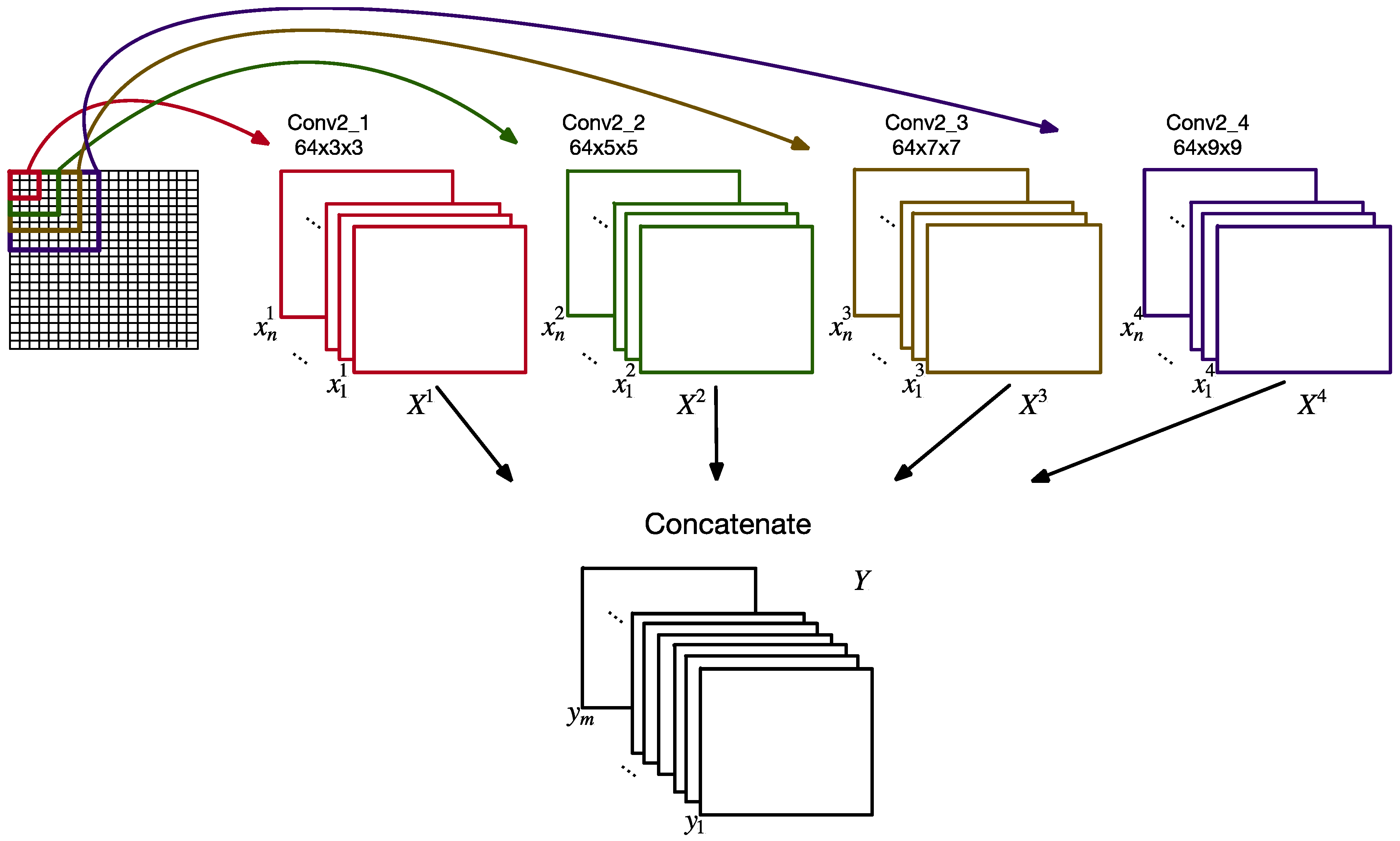
To overcome these limitations, this paper proposes a shallow multi-scale (MS) CNN with a multi-attention mechanism for bearing fault diagnosis. The time–frequency representation (TFR) as the input of the model was generated by original vibration data of the bearing. TFR bearing degradation signals are complex, nonstationary, and more effective. Zhu et al. [22] proposed an effective deep feature learning approach for remaining useful life prediction of bearings, which relied on the TFR and CNN. The TFR was applied to analyze the transients, including rapid changes in amplitude or phase during an event relative to post-event conditions [23]. TFR worked better than the vibration image used by Hoang and Kang in CNNs based on bearing fault diagnosis, which retained more comprehensive information in image data [24]. Wang et al. [25] compared eight time–frequency analysis methods for creating images, and the results indicated that continuous wavelet transform and fast Stockwell transform were the best methods for bearing diagnosis. Because of the low visual complexity of TFR images, the shallow CNN structure effectively avoids the problem of deep network training, which does not converge or overfit. MS convolutional networks were studied by Sermanet and LeCun [26], and used for recognizing traffic signs. Their research showed that the multi-scale features combined with precise details were more robust and invariant than the deep features based on the traditional CNN structure. By studying the recent literature, most of the deep learning-based fault diagnosis methods improved the depth of the network structure and the data of the training network, and they neglected the utilization efficiency of the features in the model training process. In the study of Sun et al. [27], before generating a multi-scale layer, the pooling layer and the last convolutional layer were combined, and favorable performances were obtained in a face identification task. Therefore, it can be predicted that, by keeping the global and local information synchronously, more identifiable features can be obtained between bearing health status and modes. Using the MS layer as the last convolutional layer in this study, the global and local features were sustained to increase the network capacity, allowing more scale features to be extracted for classification. Furthermore, a multi-attention mechanism was proposed to adaptively select vital features to obtain superior recognition results. Attention is an effective mechanism for selecting vital information to achieve excellent results. There are some effective attention mechanisms for image caption and machine translation, such as soft and hard attention [28], and global and local attention [29]. In this study, a deep learning model combined with the attention mechanism was adopted. The attention mechanism was used to focus on the more sensitive features of specific labels in the training process for improving the performance of model. Deep neural networks, including CNNs and recurrent neural networks, can achieve better results if they are equipped with an attention mechanism. In this paper, a multi-scale convolutional neural network (MSCNN) was combined with the multi-attention mechanism to propose a novel method for bearing fault diagnosis. The MSCNN is different from the multi-scale information in Reference [14], which was obtained from the signal before the input of the CNN; here, the multi-scale feature was obtained from the training process, combining it with the multi-attention mechanism. The proposed method achieved excellent results in simultaneously identifying the fault type and fault degree of bearings. Furthermore, the identification of specific bearing conditions was improved using the multi-attention mechanism.

2. Proposed Method

As discussed above, a shallow multi-scale convolutional neural network with multi-attention (MA-MSCNN) is proposed for bearing fault diagnosis. The TFR, as the input of the model, contains time and frequency domain information of bearing vibration data, and the TFR can effectively represent the complex and nonstationary information of bearing degradation signals [22]. Compared with the existing methods which only use the TFR to extract features manually, MSCNN can more fully mine the multi-scale information in the data for classification. Because of the low visual complexity of TFR images, the shallow structure of MA-MSCNN effectively avoids overfitting while ensuring fault diagnosis accuracy. More importantly, the proposed multi-attention mechanism allows the model to pay more attention to features which are valuable for classification, and, based on the experimental results in Section 3, the effectiveness of the model for fault identification was further improved. Firstly, the samples were generated by enhanced sampling [30]. Then, 1D vibration data were converted to two-dimensional TFR image data via continuous wavelet transform. Because the frequency range of the vibration data was broad, and the size of the generated TFR image was huge, the bilinear interpolation method was used to reduce the size of the TFR. The resized TFR image was used as the input of MA-MSCNN. During the training process, the parameters were updated using the Adam optimizer. The procedure of the proposed method is illustrated in Figure 1.

2.1. Time–Frequency Representation

Firstly, samples were generated by improved sampling, and the enhanced sampling as a data augmentation technology is shown in Figure 2. Samples were sampled in the vibration data of each health condition, and each degree represented the damage by enhanced sampling. Then, each sample was converted to 2D image data. Compared with the time–frequency image obtained by short-time Fourier transform, the time–frequency image obtained by wavelet transform is better [17], because the resolution of wavelet transform at high frequency can be adjusted automatically, and the resolution of the TFR image obtained is higher. It has a sinusoidal basis function, which is different from Fourier transform. In wavelet transform, the signal can be decomposed into different resolutions in different time and space scales by transforming and scaling the wavelet basis function. The reason why this operation can be performed is due to the limited width of the time domain and frequency domain of the wavelet basis function used in the wavelet transform. Monitoring rotating machinery conditions is one of its main application fields [31]. A new concept of wavelet was firstly proposed, and then continuous wavelet transform was applied as shown below.

$${\mathsf{\Psi }}_{\alpha ,\beta }\left(t\right)={\left|\alpha \right|}^{-\frac{1}{2}}\mathsf{\Psi }\left(\frac{t-\beta }{\alpha }\right);\alpha ,\beta \in R, \alpha \ne 0,$$

(1)

$$\mathrm{U}\left(\alpha ,\beta \right)={{\displaystyle \int }}_{-\infty }^{\infty }x\left(t\right){\mathsf{\Psi }}_{\alpha ,\beta }\left(t\right)dt,$$

(2)

$$\mathrm{U}\left(\alpha ,\beta \right)={{\displaystyle \int }}_{-\infty }^{\infty }x\left(t\right){\left|\alpha \right|}^{-\frac{1}{2}}\mathsf{\Psi }\left(\frac{t-\beta }{\alpha }\right)dt,$$

(3)

where $\alpha$ is the scaling parameter, $\beta$ is the translating parameter, and $\mathsf{\Psi }\left(t\right)$ is a continuous wavelet, the shape and displacement of which are determined by $\alpha$ and $\beta$, respectively. The Morlet wavelet, similar to the impulse signal of rotating machinery, was chosen as the mother wavelet, due to the lack of a standard or general method to select mother wavelets [32], where $\mathrm{U}(·)$ is the wavelet 2D coefficient of the 1D degradation signal $x\left(t\right)$, which is the time–frequency representation (TFR).

The TFR images were generated from all the samples by continuous wavelet transform through Equations (1)–(3). In order to illustrate the variation of frequency energy with different health conditions and the variation of frequency energy with time, TFR images of each label are given in Figure 3. When the bearing was in a normal condition, the rotation frequency was apparent in the TFR image, and the frequency fluctuation was not evident. However, in the conditions of faults on the testing bearings at the inner raceway, outer raceway, and ball, the bearings under defect conditions had periodic impact phenomena, causing the effect of modulation.

2.2. Dimensionality Reduction (Image Resize)

The vibration data of the testing bearing were collected by an accelerometer with a sampling frequency of 12 kHz, and the vibration signal included a frequency range of 0–6000 Hz. The size of the original generated TFR image was 1000 × 6000, and we needed to reduce the dimensions due to the high-dimensional features of these TFRs. Instead of using general approaches such as principal component analysis (PCA) and nearest-neighbor interpolation, a simple and effective method was introduced, named bilinear interpolation, which was effectively applied in image processing [33]. The bilinear interpolation performed a linear interpolation operation in two directions, making full use of the actual pixel values in the source image to determine the pixel value in the target image. Therefore, it had a much better scaling effect than the simple nearest-neighbor interpolation.

Figure 4 shows that $Q_{1,1}$, $Q_{1,2}$, $Q_{2,1}$, and $Q_{2,2}$ were the four pixels in the original image, and the corresponding positions were $\left(x_1,y_1\right)$, $\left(x_1,y_2\right)$, $\left(x_2,y_1\right)$, and $\left(x_2,y_2\right)$; $\mathrm{P}\left(x,y\right)$ was the result of the pixels resized, as shown below.

$$f\left(R_1\right)\approx \frac{x_2-x}{x_2-x_1}f\left(Q_{1,1}\right)+\frac{x-x_1}{x_2-x_1}f\left(Q_{2,1}\right),$$

(4)

$$f\left(R_2\right)\approx \frac{x_2-x}{x_2-x_1}f\left(Q_{1,2}\right)+\frac{x-x_1}{x_2-x_1}f\left(Q_{2,2}\right),$$

(5)

$$f\left(P\right)\approx \frac{y_2-y}{y_2-y_1}f\left(R_1\right)+\frac{y-y_1}{y_2-y_1}f\left(R_1\right).$$

(6)

These TFR images were resized to 28 × 28 to train the MA-MSCNN model using bilinear interpolation through Equations (4)–(6); the resized image of one TFR image is shown in Figure 5.

2.3. Multi-Scale Convolutional Neural Network (MSCNN)

Classification in related fault diagnosis based on CNNs only uses the features of the last layer. Thus, many detailed pieces of information in the inter-layers are lost through these feature flows. Inspired by LeCun [26], the MS convolutional layer was proposed aiming to keep the global and local information to increase the network capacity. The MS layer combined multiple convolution kernels of different sizes in the same convolutional layer. The resulting MS convolutional feature map was mixed, then passed to the next pooling layer for subsampling, and imposed to the fully connected layer; finally, the result was obtained through the output layer by softmax.

After the convolution of the kernels and the input image, local features were formed in a convolutional layer, and then a nonlinear activation function was imposed. A three-dimensional tensor, containing a stack of matrices called feature maps, was the output of the convolutional layer. The representation of the output feature map in the convolutional layer is shown below.

$$Y_j^T=\phi \left({\displaystyle \sum }_{i=0}^n{\omega }_{ij}^T\ast Y_j^{T-1}+b_j^T\right),$$

(7)

where the $\ast$ operator was used for the 2D convolution of the channel., In this convolution operation, $Y_j^{T-1}$ is the j-th input tensor of layer T − 1, and $Y_j^T$ is the j-th output tensor of layer T; $b_j^T$ is the weight of convolution bias, while ${\omega }_{ij}^T$ is the weight of convolution kernel; $\phi (·)$ is a nonlinear activation function with, which the final output can be achieved.

In the traditional neural network, the high-level feature obtained by the last convolution layer after the layer-by-layer convolution operation is used for the final task fitting, and the high-level feature tends to be stable after multi-layer convolution. In some cases, some detailed low-level features may be overlooked. The MS layer of MA-MSCNN was combined for convolution kernels on different scales in the second convolutional layer before the formation of a mixed layer. The mixed layer helped the net to learn higher-level features and low-level features, in order to represent the image features with fewer neurons. The MS layer is illustrated in Figure 6. The output of the mixed layer can be written as

$$Y=\phi \left({\displaystyle \sum }_{i=0}^{n_1}{\omega }_{ij}^1\ast x_i^1+{\displaystyle \sum }_{i=0}^{n_2}{\omega }_{ij}^2\ast x_i^2+{\displaystyle \sum }_{i=0}^{n_3}{\omega }_{ij}^3\ast x_i^3+{\displaystyle \sum }_{i=0}^{n_4}{\omega }_{ij}^4\ast x_i^4+b_j\right),$$

(8)

where $x_i^1,{\omega }_{ij}^1$, $x_i^2,{\omega }_{ij}^2$, $x_i^3,{\omega }_{ij}^3$, and $x_i^4,{\omega }_{ij}^4$ denote the neurons and weights from the kernels of the multi-scale convolution layer, whereas $n_i$ means there are n filters in $\mathrm{Conv}2\_i$. Y, as the output of the mixed layer, is sent into the next layer. The size of all feature maps remains the same, as they are fed into the attention module, which requires the same size for multi-scale features.

2.4. Multi-Attention Mechanism

2.4.1. Spatial Attention

According to the TFR image of the bearing vibration data, partial regions of the image corresponded to the different fault types, which were observed by the spatial attention mechanism. $Y_{W\times H}$ represents the output of a feature map from the MC layer. The width (W) and height (H) were unfolded to reshape $Y_{W\times H}$ into a vector $\left(y_1, y_2, \dots ,y_m\right)$ in which $m=W\times H$. Here, $y_i$ was regarded to be the feature of the i-th location. The single-layer neural network and softmax function were applied successively on the image area to form the attention distribution. The attention distribution α was generated by a multi-layer perceptron and a softmax function. The spatial attention model ${\mathsf{\varphi }}_s$ can be defined as

$${\alpha }_i=softmax\left(\phi \left({\omega }_i{y}_i+b_i\right)\right),$$

(9)

where ${\omega }_i$ and $b_i$ are the weight and bias of model. After the spatial attention weights (${\alpha }_i$) were generated through Equation (9), the feature was represented as a vector $\left({\alpha }_1{y}_1,{\alpha }_2{y}_2, \dots , {\alpha }_m{y}_m\right)$ by element multiplication. Finally, the obtained feature vectors were reshaped into $Y_{W\times H}^{\prime }$.

2.4.2. Channel-Based Attention

Spatial attention from the visual feature V was not the basis of attention. The feature V in this study was analyzed by introducing a channel-based attention mechanism. Notably, the mode detectors were provided by the CNN filters, and the response of the corresponding convolution filter could activate the feature map channel in the CNN. Therefore, the application of the attention mechanism in channel mode could be regarded as a way to select the most sensitive feature channel for fault recognition. As shown in Figure 6, $Y=\left[y_1, y_2, \dots ,y_m\right]$ were the feature maps generated from the previous layer, where $y_j$ is the j-th channel of the feature maps $Y$, and $\mathrm{m}$ is the total number of channels. The channel attention model ${\mathsf{\varphi }}_c$ can be defined after the definition of the spatial attention model, which is shown below.

$${\beta }_j=softmax\left(\phi \left({\omega }_j{y}_j+b_j\right)\right),$$

(10)

where ${\beta }_j$ is the channel-wise attention weight, and ${\omega }_j$ and $b_j$ are weight and bias terms. The final representation $Y_{atten}$ and channel attention weights ${\beta }_j$ can be defined as follows:

$$Y_{atten}=\left[y_1^{\prime },y_2^{\prime }, \dots , y_m^{\prime }\right],$$

(11)

$${\mathrm{y}}_j^{\prime }={\displaystyle \sum }_{j=1}^m{\beta }_j{y}_j.$$

(12)

In addition to using channel attention and spatial attention separately, there were two kinds of models according to the different realization order of the two attention mechanisms, which combined the two attention mechanisms. The first type, SC-Attention, applied spatial attention before channel-wise attention. The second type, denoted as CS-Attention, was the model with spatial attention implemented first. All training objectives were to minimize the cross-entropy loss. The effects of the two models on the results of fault diagnosis are also compared in the experimental analysis.

2.5. MA-MSCNN Training

The topology of the MA-MSCNN is shown in Figure 7. The classification layer after multi-attention was a two-layer fully connected multi-layer perceptron with rectified linear unit (ReLU) activation function and softmax output, and the dropout layer with a 50% rate was set between the two fully connected layers to prevent overfitting. Features can be aggregated in different locations of feature mapping through the pooling layer following the convolution layer. The convolution feature dimensions of convolution layers can also be reduced through pooling; as the size of the feature graph decreases, the computational efficiency is improved. Max-pooling was employed, which is given as

$$Y_j^T\left(m,n\right)=\underset{0\le p,q<s}{\max }\left\{Y_j^{T-1}\left(m·s+p, n·s+q\right)\right\},$$

(13)

where $Y_j^{T-1}$ and $Y_j^T$ are the j-th input tensor of layer T − 1 and layer T, and the pooling size is $\mathrm{s}\times \mathrm{s}$. At last, the fully connected layer enables the expansion of the output of the last pooling layer to be the input of the softmax layer for diagnosis. In this process, the cross-entropy lies between the true label and the estimated softmax output, which is the loss function of MA-MSCNN, defined as

$$J\left(\theta ;f,\rho \right)=-\frac{1}{m}{\displaystyle \sum }_{i=0}^m{\rho }^{\left(i\right)}\log \left[h_{\theta }\left(f^{\left(i\right)}\right)\right]+\left(1-y^{\left(i\right)}\right)log\left[1-h_{\theta }\left(f^{\left(i\right)}\right)\right],$$

(14)

where $f$ is the expanding feature in the last layer, and $\mathsf{\rho }$ is the desired output for diagnosis; $h_{\theta }$ is the regression function for result predicting, and $\mathsf{\theta }=\left\{\omega ,\mathrm{b}\right\}$ denotes the parameters of the function. There are many similarities between traditional CNN and other parts of MA-MSCNN. The initialization of the weights and biases for all layers was carried out firstly in the training of MA-MSCNN. In order to minimize the loss function when the learning rate was 0.001, the Adam optimizer was used to optimize the parameter set θ of MA-MSCNN. A learning rate too high or too low may result in training divergence or slow convergence, respectively, neither of which are favorable. Generally, in order to ensure the speed and stability of training, repeated experiments in training were used to determine the appropriate learning rate. The random division of the training samples into several small batches, containing 16 samples in each batch, was carried out in each epoch. Then, they were put into the network. The details of the architecture of MA-MSCNN are shown in

Table 1. The details of the architecture of the shallow multi-scale convolutional neural network with multi-attention (MA-MSCNN).

Layer	Parameter	Value	Output size
Input layer	-	-	$28\times 28$
C1	Kernels	$7\times 7\times 32$	$28\times 28\times 32$
	Strides	1
	Padding	Same
P1	Ksize	$2\times 2$	$14\times 14\times 32$
	Strides	2
MS layer	Kernel_1	$3\times 3\times 64$	$14\times 14\times 256$
	Kernel_2	$5\times 5\times 64$
	Kernel_3	$7\times 7\times 64$
	Kernel_4	$9\times 9\times 64$
	Strides	1
	Padding	Same
P2	Ksize	$2\times 2$	$7\times 7\times 256$
	Strides	2
F1	neurons	1024	$1024\times 1$
Dl	Dropout rate	50%	-
F2	neurons	1024	$1024\times 1$

.

The multi-scale features [26] and deep hidden identity features [27] showed that the last convolutional layer had more constant and robust deep features (global information) than the low-level layers, making it suitable for “large data” in complex operating conditions. Many precise details (local information) contained in low-level features which are sensitive to interference would be partially lost in high-level layers, which is unfavorable for the dissemination of information in the network. In this case, by inputting the multi-scale convolution result of the last convolution layer in the fully connected layer, the global and local features could be preserved simultaneously, making the classification more accurate. The topology of the MA-MSCNN proposed is shown in Figure 7. The feature maps of C1 were the outputs of the C1 layer using 32 filters. The multi-scale feature maps concatenated conv2_1, conv2_2, conv2_3, and conv2_4 generated by the MS-layer, as shown in Figure 6. The attention feature maps were generated using the attention mechanism described in Section 2.4. From the channel attention feature maps shown in Figure 8, when the color of the feature channel is darker, the channel attention weight ${\beta }_j$ in Equation (10) is larger, which means that the channel of feature is more sensitive for fault recognition. Lighter colors have the opposite effect. In the spatial attention feature maps, the darker part represents a larger spatial attention weight ${\alpha }_i$ in Equation (9), which means that, in each feature map, the information in this area is more relevant to the true label of the sample. The reweighted feature maps using the attention mechanism pay more attention to the features related to bearing health condition.

2.6. MA-MSCNN Fault Diagnosis

The original vibration data were cut into samples of the same size by enhanced sampling, and then the samples were labeled and divided into a training set and test set. The vibration data sample was converted into a cropped TFR to construct the input of the MA-MSCNN. The detected fault condition came from the result of fault detection, which was also the output of the model.

3. Experimental Verification

A series of experiments were carried out to evaluate the effectiveness of the proposed bearing fault diagnosis method. The Bearing Data Center of Case Western Reserve University provided experimental data for multiple faults [34]. Single point faults of 0.007, 0.014, and 0.021 inches were distributed on the rolling parts, and the inner and outer rings of drive end bearings, respectively. In the experiment, there were four load conditions, including 0, 1, 2, and 3 hp. The vibration generated in the test was measured at 12-kHz sampling frequency. According to the proposed method, fault type and fault degree could be separated simultaneously. The damage degree of the bearing was indicated by the fault sizes of 0.007, 0.014, 0.021, and 0.028 inches. Twelve kinds of bearing health conditions under four kinds of loads were included in the dataset, among which the same health conditions under different loads were divided equally.

Table 2. The labels of data with different fault types and different degrees.

Fault Degree	Inner	Ball	Outer	Normal
0.007	I-07	B-07	O-07	N-00
0.014	I-14	B-14	O-14
0.021	I-21	B-21	O-21
0.028	I-28	B-28	-

shows the 12 data labels from different fault types and different fault degrees. Samples were obtained in the vibration data of each health condition by enhanced sampling. Each sample contained 1000 points, and the stride of enhanced sampling was 100. Therefore, each dataset contained 4360 samples. In total, 70% of the 17,440 samples were used as training samples and 30% were used as test samples. 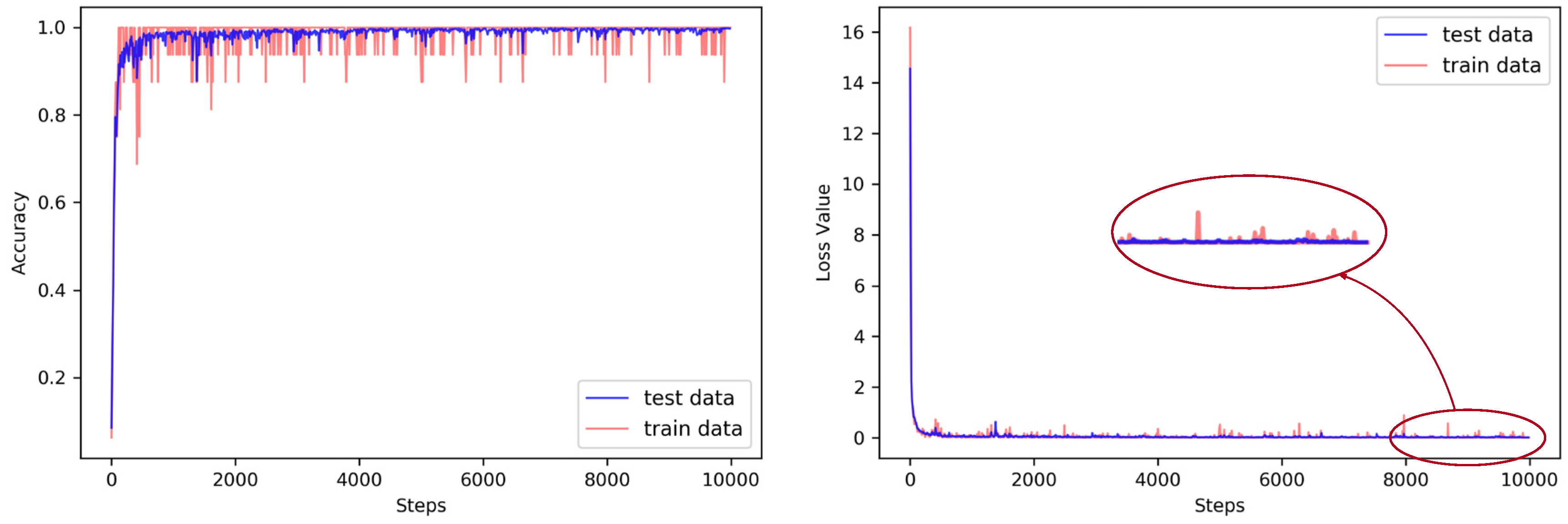Figure 9 shows that the loss value and accuracy of the proposed MA-MSCNN tended to stabilize during the training steps of 8000 to 10,000. Thus, in the experiment, the number of training steps was determined to be 10,000 steps. The model was built by TensorFlow (1.8.0) and was only completed by central processing unit (CPU) training. The training time was nearly six hours on a laptop computer (64-bit, i7 7700HQ 2.8-GHz CPU, 16 GB random-access memory (RAM)).

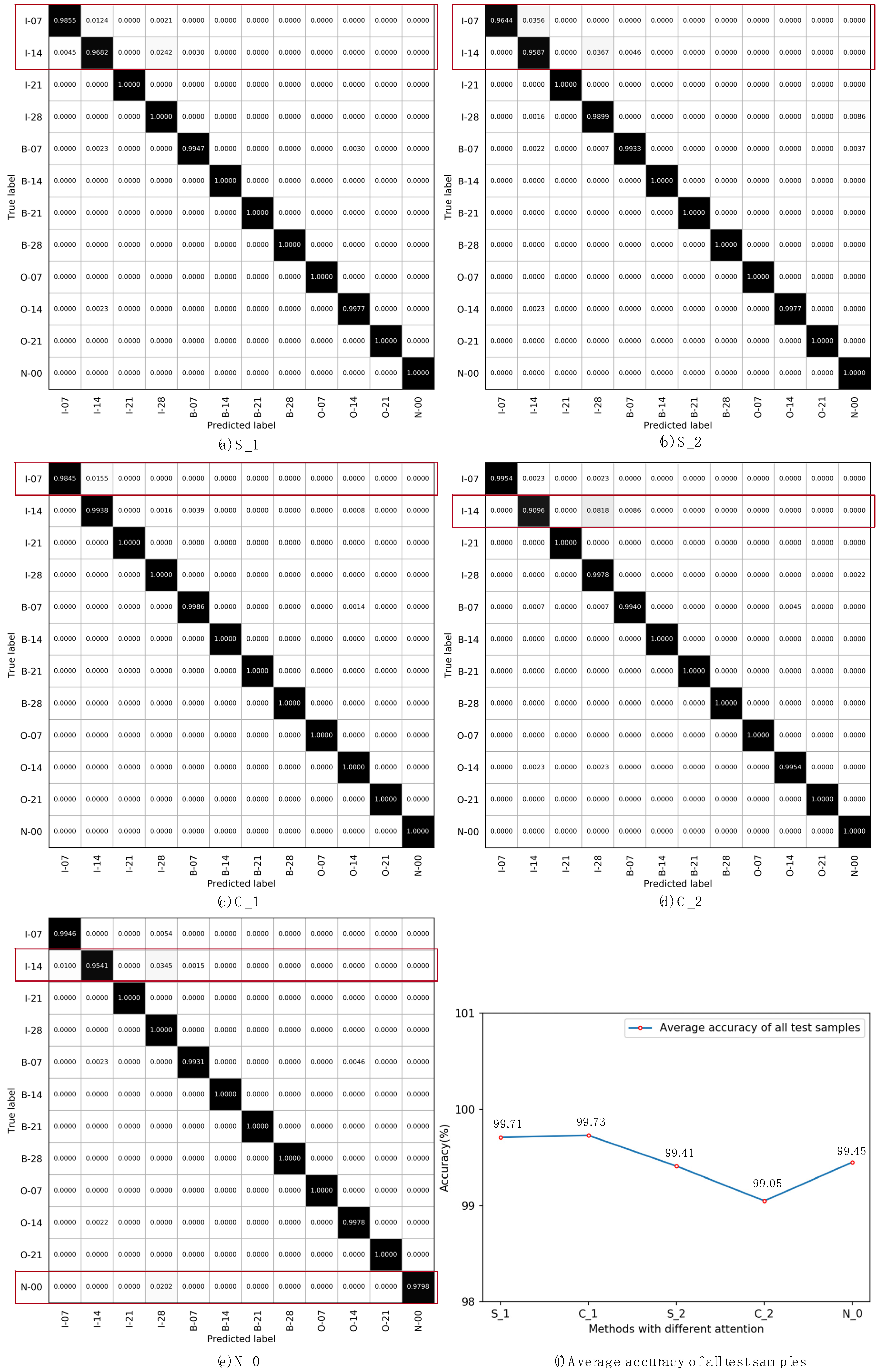
3.1. Evaluations of Single Attention

In this section, the comparison of a single kind of attention mechanism with the multi-scale CNN is evaluated. S_1 was a pure spatial attention mechanism followed by the first convolution layer (C1). After getting the spatial attention weights from the attention mechanism, we combined it with the feature maps of the C1 layer through element multiplication and fed it into the next layer. S_2 was a pure spatial attention mechanism followed by the MS layer. Then, the spatial weighted feature maps were fed into the next layer for classification. C_1 was a pure channel-based attention mechanism followed by the first convolution layer (C1). After getting the channel attention weights from the attention mechanism, we combined it with the feature maps of the C1 layer using Equations (11) and (12) and fed it into the next layer. C_2 was a pure channel-based attention mechanism followed by the MS layer. Then, the channel weighted feature maps were fed into the next layer for classification. N_0 was the MSCNN without an attention mechanism, and the architecture was similar to the multi-attention layer removed in Figure 7.

According to the statistics during the experiment, there were a total of 51,124 valid samples participating in this section of the validation, of which 35,787 were for training, and 15,337 were for testing. All the results are reported in Figure 10. The identification of each faulty label in each method is represented in the form of a confusion matrix. According to the results from Figure 10, we can make a few observations. Firstly, from the average recognition accuracy, shown in Figure 10f, by identifying all the test samples, we can see that the fault recognition ability of the model was improved by setting the single attention mechanism followed by the first convolution layer (C1). Secondly, from the confusion matrix shown in Figure 10a–e, we can see that the single attention mechanism had an impact on the recognition of the specific condition of the bearing, and the accuracy of normal condition (N_0) recognition was significantly improved by the model. Thirdly, from the recognition results, the identification of the label I-14 sample using the single attention mechanism was not improved, and the sample identification accuracy of the label I-07 was even reduced.

3.2. Evaluations of Multi-Attention

Depending on the order of implementation of channel-based attention and spatial attention, there were two types of models that combined the two attention mechanisms. The distinction between these two types is shown in Figure 11. The first type, named the SC-Attention mechanism, applied spatial attention before channel-based attention. Firstly, initial feature map $V^l$ was given, and the spatial attention weight ${\alpha }^l$ was obtained by using the spatial attention ${\mathsf{\varphi }}_s$. The spatial weighted feature maps were obtained by the linear combination of ${\alpha }^l$ and $V^l$. Then, the spatial weighted feature maps were input into the channel-based attention model ${\mathsf{\varphi }}_c$ to receive the channel attention weight ${\beta }^l$. Finally, the channel attention weights ${\beta }^l$ and feature maps after spatial attention were multiplied in the channel dimension to get the final feature $X^l$. The second type, denoted as the CS-Attention mechanism, was a model with the channel-based attention implemented first. For the CS-Attention mechanism, given the initial feature map $V^l$, the channel attention weight ${\beta }^l$ was firstly obtained using the channel-based attention ${\mathsf{\varphi }}_c$. Then, the channel weighted feature maps were input into the spatial attention model ${\mathsf{\varphi }}_s$ to obtain the spatial attention weight ${\alpha }^l$. Finally, feature maps $X^l$ were obtained by multiplying the spatial weights ${\alpha }^l$ and the feature maps after channel attention in the spatial dimension.

In this section, the comparisons of MA-MSCNN with different kinds of multi-attention mechanisms are evaluated. SC_1 was the SC-Attention mechanism followed by the first convolution layer (C1). The feature maps after multi-attention mechanism were fed into the next layer. CS_1 was the SC-Attention mechanism followed by the first convolution layer (C1). SC_2 was the SC-Attention mechanism followed by the MS layer. Then, the attention weighted feature maps were fed into the next layer for classification. CS_2 was the CS-Attention mechanism followed by the MS layer. The results of these four comparisons are shown in Figure 12. According to the results from Figure 12, we can make a few observations. Firstly, from the average recognition accuracy, shown in Figure 12e, by identifying all the test samples, we can see that the multi-attention mechanism after a multi-scale convolutional layer (MS-Layer) is better than a single attention mechanism. This shows that the MA-MSCNN model combined with the multi-scale convolutional layer and the multi-attention mechanism proposed in this paper is more effective in bearing fault diagnosis. Secondly, by using the multi-attention mechanism, the ability of the model to identify individual fault types was also improved. It can be seen from the experimental results that the identification of fault labels I-07 and I-14 was not excellent using the single attention mechanism, and the recognition accuracy of the two fault labels was significantly improved by the multi-attention mechanism.

Table 3. Recognition accuracy of fault labels I-07 and I-14 using single attention mechanisms.

	S_1	S_2	C_1	C_2	N_0
I-07	98.55	96.44	98.45	99.54	99.46
I-14	96.82	95.87	99.38	90.96	95.41

and

Table 4. Recognition accuracy of fault labels I-07 and I-14 using multi-attention mechanisms.

	SC_1	SC_2	CS_1	CS_2
I-07	99.35	99.14	99.89	99.77
I-14	98.24	99.23	97.67	99.38

show the identification results for different situations using the single attention mechanism and the multi-attention mechanism, respectively. Comparing Table 3 and Table 4, the results show clearly that the model with the multi-attention mechanism had better diagnosis accuracies for labels I-07 and I-14 than the model with the single attention mechanism.

Table 5. Recognition results for different fault degrees.

Type	Inner				Ball				Outer			Normal
Fault degree	0.007	0.014	0.021	0.028	0.007	0.014	0.021	0.028	0.007	0.014	0.021	-
No. samples	4360	4360	4360	4360	4360	3266	4359	4360	4360	4359	4260	4360
Accuracy (%)	99.14	99.23	100	99.92	99.63	100	100	100	100	99.70	100	100

shows the recognition results of the different fault degrees under each fault type. It can be seen that the diagnosis method proposed in this paper can also perform well in the case of a small difference in fault degree.

4. Comparison with Related Works

As a common method in the study of mechanical fault diagnosis, the rolling bearing dataset used in this investigation is very popular. Many excellent classification results were reported in recent years (95%) and higher testing accuracies were achieved in References [9,14,15,21]. However, when studying the existing methods for this dataset, it was found that the accuracy of the current intelligent diagnosis reached a ceiling. Most studies focused on the input data and the structure of model, whereas very limited work could be found on efficiently mining multi-scale features using the attention mechanism.

In the latter case, a testing accuracy of 97.91% was obtained in Reference [9] using optimized support vector machines. The model was trained by 880 samples, and the number of test samples was 1320. Then, 1000 test samples were divided into 11 classes with different fault types and degrees. An improved multi-scale cascade CNN (MC-CNN) was proposed in Reference [14] to mine multi-scale features of input signals. This study focused on the input data of the CNN, and the multi-scale information was obtained in the input layer to improve the performance of the CNN. Only four bearing conditions were classified, and 99.61% testing accuracy was obtained based on 50 experiments. The 800 samples used in the experiment were divided into training sets and testing sets according to three proportions, and the model had the best testing accuracy when the training set had the largest number of samples. Ten bearing conditions were considered in Reference [15], and 20,000 samples were obtained via data augmentation. As a result, as high as 98.8% classification accuracy was achieved from 2500 testing samples. In Reference [21], a two-stage machine learning method based on unsupervised feature learning and sparse filtering was proposed. The experimental dataset contained 4000 samples, and a fairly high identification accuracy of 99.66% was obtained when 10% of samples were used for training.

The method proposed in this paper allowed achieving an accuracy of bearing fault diagnosis as high as 99.86%. The MSCNN model with a multi-scale attention mechanism provided higher recognition accuracy, as shown in Figure 11e. This study carried out a more detailed condition segmentation using the same dataset obtained from Case Western Reserve University. Considering 12 bearing health conditions, the trained model identified 15,337 testing samples. A detailed study on the comparisons of classification accuracy with other researches on the same bearing dataset with diagnosis accuracy higher than 95% is shown in

Table 6. Comparisons of classification accuracy of other researches on the same bearing dataset.

Models	Method	Number of Fault Classes	Testing Accuracy
ICDSVM	[9]	11	97.91%
MC-CNN	[14]	4	99.61%
FMCNN	[15]	10	98.8%
Unsupervised learning	[21]	10	99.66%
MA-MSCNN	Proposed	12	99.86%

.

5. Conclusions

In this paper, a novel multi-scale convolutional neural network with a multi-attention model, dubbed MA-MSCNN, was proposed for bearing fault diagnosis. MA-MSCNN combines multi-scale convolutional layers with a multi-attention mechanism to optimize the model’s use of multi-scale information to achieve advanced good performance in intelligent bearing fault diagnosis. Since there is an MS layer in the MA-MSCNN, both global and local features can be preserved. Then, attentive features generated by a multi-attention mechanism allow the better utilization of label-related information in classification. Comprehensive experiments were carried out to evaluate the value of the attention mechanism. Different kinds of single attention mechanisms and multi-attention mechanisms were compared. We found that the multi-attention mechanism could effectively improve the diagnosis accuracy by paying more attention to the features valuable for classification. A comparison with other methods and related studies was provided to verify the superiority of the proposed method. The results showed that samples of different fault types and degrees were well distinguished by this method. Furthermore, the method proposed in this paper effectively improved the accuracy of data identification of the I-14 label, which was a problem present in Reference [9]. This reveals that the proposed method can diagnose bearing faults more effectively with varying loads.

In future work, two points need to be addressed. Firstly, the experimental data were collected from a stable environment, and actual working environments are more complicated. Therefore, in future work, we will collect fault data in actual work environments and further evaluate the performance of the proposed model. Secondly, we will develop a real-time fault diagnosis system based on the method proposed in this paper.

References

1. Rai, A.; Upadhyay, S. A review on signal processing techniques utilized in the fault diagnosis of rolling element bearings. Tribol. Int. 2016, 96, 289–306. [Google Scholar] [CrossRef]
2. Sun, C.; Zhang, Z.; He, Z.; Shen, Z.; Chen, B.; Xiao, W. Novel method for bearing performance degradation assessment—A kernel locality preserving projection-based approach. Proc. Inst. Mech. Eng. Part C J. Mech. Eng. Sci. 2014, 228, 548–560. [Google Scholar] [CrossRef]
3. Yu, J. Bearing performance degradation assessment using locality preserving projections and Gaussian mixture models. Mech. Syst. Signal Process. 2011, 25, 2573–2588. [Google Scholar] [CrossRef]
4. Tian, J.; Morillo, C.; Azarian, M.H.; Pecht, M. Motor bearing fault detection using spectral kurtosis-based feature extraction coupled with K-nearest neighbor distance analysis. IEEE Trans. Ind. Electron. 2016, 63, 1793–1803. [Google Scholar] [CrossRef]
5. Yang, Y.; Yu, D.; Cheng, J. A roller bearing fault diagnosis method based on EMD energy entropy and ANN. J. Sound Vib. 2006, 294, 269–277. [Google Scholar]
6. Nikolaou, N.G.; Antoniadis, I.A. Rolling element bearing fault diagnosis using wavelet packets. Ndt E Int. 2009, 35, 197–205. [Google Scholar] [CrossRef]
7. Yang, Y.; Yu, D.; Cheng, J. A fault diagnosis approach for roller bearing based on IMF envelope spectrum and SVM. Measurement 2007, 40, 943–950. [Google Scholar] [CrossRef]
8. Yang, J.; Zhang, Y.; Zhu, Y. Intelligent fault diagnosis of rolling element bearing based on SVMs and fractal dimension. Mech. Syst. Signal Process. 2007, 21, 2012–2024. [Google Scholar] [CrossRef]
9. Zhang, X.; Liang, Y.; Zhou, J.; Zang, Y. A novel bearing fault diagnosis model integrated permutation entropy, ensemble empirical mode decomposition and optimized SVM. Measurement 2015, 69, 164–179. [Google Scholar] [CrossRef]
10. Ince, T.; Kiranyaz, S.; Eren, L.; Askar, M.; Gabbouj, M. Real-time motor fault detection by 1-D convolutional neural networks. IEEE Trans. Ind. Electron. 2016, 63, 7067–7075. [Google Scholar] [CrossRef]
11. Peng, D.; Liu, Z.; Wang, H.; Qin, Y.; Jia, L. A Novel Deeper One-Dimensional CNN with Residual Learning for Fault Diagnosis of Wheelset Bearings in High-Speed Trains. IEEE Access 2019, 7, 10278–10293. [Google Scholar] [CrossRef]
12. Eren, L.; Ince, T.; Kiranyaz, S. A generic intelligent bearing fault diagnosis system using compact adaptive 1D CNN classifier. J. Signal Process. Syst. 2019, 91, 179–189. [Google Scholar] [CrossRef]
13. Guo, L.; Lei, Y.; Xing, S.; Yan, T. Deep convolutional transfer learning network: A new method for intelligent fault diagnosis of machines with unlabeled data. IEEE Trans. Ind. Electron. 2019, 66, 7316–7325. [Google Scholar] [CrossRef]
14. Huang, W.; Cheng, J.; Yang, Y.; Guo, G. An improved deep convolutional neural network with multi-scale information for bearing fault diagnosis. Neurocomputing. 2019, 359, 77–92. [Google Scholar] [CrossRef]
15. An, F.P. Rolling bearing fault diagnosis algorithm based on FMCNN-Sparse representation. IEEE Access 2019, 7, 102249–102263. [Google Scholar] [CrossRef]
16. Guo, X.; Chen, L.; Shen, C. Hierarchical adaptive deep convolution neural network and its application to bearing fault diagnosis. Measurement. 2016, 93, 490–502. [Google Scholar] [CrossRef]
17. Li, X.; Ding, Q.; Sun, J.Q. Remaining useful life estimation in prognostics using deep convolution neural networks. Reliab. Eng. Syst. Saf. 2018, 172, 1–11. [Google Scholar] [CrossRef] [Green Version]
18. Janssens, O.; Slavkovikj, V.; Vervisch, B.; Stockman, K.; Loccufier, M.; Verstockt, S.; Van Hoecke, S. Convolutional neural network based fault detection for rotating machinery. J. Sound Vib. 2016, 377, 331–345. [Google Scholar] [CrossRef]
19. Guo, S.; Yang, T.; Gao, W.; Zhang, C. A Novel Fault Diagnosis Method for Rotating Machinery Based on a Convolutional Neural Network. Sensors 2018, 18, 1429. [Google Scholar] [CrossRef]
20. Udmale, S.S.; Patil, S.S.; Phalle, V.M.; Singh, S.K. A bearing vibration data analysis based on spectral kurtosis and ConvNet. Soft Comput. 2019, 23, 9341–9359. [Google Scholar] [CrossRef]
21. Lei, Y.; Jia, F.; Lin, J.; Xing, S.; Ding, S.X. An intelligent fault diagnosis method using unsupervised feature learning towards mechanical big data. IEEE Trans. Ind. Electron. 2016, 63, 3137–3147. [Google Scholar] [CrossRef]
22. Zhu, J.; Chen, N.; Peng, W. Estimation of bearing remaining useful life based on multiscale convolutional neural network. IEEE Trans. Ind. Electron. 2019, 66, 3208–3216. [Google Scholar] [CrossRef]
23. Negi, S.S.; Kishor, N.; Kumar, A.; Uhlen, K. Signal Processing for TFR of Synchro-phasor data. IET Gener. Transm. Distrib. 2017, 11, 3881–3891. [Google Scholar] [CrossRef]
24. Hoang, D.T.; Kang, H.J. Convolutional Neural Network Based Bearing Fault Diagnosis. In Proceedings of the 13th International Conference on Intelligent Computing (ICIC), Liverpool, UK, 7–10 August 2017; pp. 105–111. [Google Scholar]
25. Wang, J.; Mo, Z.; Zhang, H.; Miao, Q. A Deep Learning Method for Bearing Fault Diagnosis Based on Time-Frequency Image. IEEE Access 2019, 7, 42373–42383. [Google Scholar] [CrossRef]
26. Sermanet, P.; LeCun, Y. Traffic sign recognition with multi-scale convolutional networks. In Proceedings of the 2011 International Joint Conference on Neural Networks, San Jose, CA, USA, 31 July–5 August 2011; pp. 2809–2813. [Google Scholar]
27. Sun, Y.; Wang, X.; Tang, X. Deep learning face representation from predicting 10000 classes. In Proceedings of the 27th IEEE Conference on Computer Vision and Pattern Recognition (CVPR), Columbus, OH, USA, 24–27 June 2014; pp. 1891–1898. [Google Scholar]
28. Xu, K.; Ba, J.; Kiros, R.; Cho, K.; Courville, A.; Salakhudinov, R.; Bengio, Y. Show, attend and tell: Neural image caption generation with visual attention. In Proceedings of the International conference on machine learning, Lille, France, 6–11 July 2015; pp. 2048–2057. [Google Scholar]
29. Luong, M.T.; Pham, H.; Manning, C.D. Effective approaches to attention-based neural machine translation. arXiv 2015, arXiv:1508.04025. [Google Scholar]
30. Zan, T.; Wang, H.; Wang, M.; Liu, Z.; Gao, X. Application of multi-dimension input convolutional neural network in fault diagnosis of rolling bearings. Appl. Sci. 2019, 9, 2690. [Google Scholar] [CrossRef]
31. Grossmann, A.; Morlet, J. Decomposition of Hardy functions into square integrable wavelets of constant shape. SIAM J. Math. Anal. 1984, 15, 723–736. [Google Scholar] [CrossRef]
32. Tang, B.; Liu, W.; Song, T. Wind turbine fault diagnosis based on Morlet wavelet transformation and Wigner-Ville distribution. Renew. Energy 2010, 35, 2862–2866. [Google Scholar] [CrossRef]
33. Raveendran, H.; Thomas, D. Image fusion using LEP filtering and bilinear interpolation. Int. J. Eng. Trends Technol. 2014, 12, 427–431. [Google Scholar] [CrossRef]
34. Bearing Data Center. Available online: http://csegroups.case.edu/bearingdatacenter/pages/download-data-file (accessed on 16 March 2017).
Figure 1. Framework of the proposed fault diagnosis method and structure of the multi-scale convolutional neural network with a multi-attention mechanism.
Energies 12 03937 g001
Figure 2. The samples generated by enhanced sampling.
Energies 12 03937 g002
Figure 3. The vibration signal converted to a time–frequency representation (TFR) image by continuous wavelet transform: (a) waveform for the sample in normal conditions; (b) TFR image for the sample in normal conditions; (c) waveform for the sample with an inner raceway fault; (d) TFR image for the sample with an inner raceway fault; (e) waveform for the sample with a ball fault; (f) TFR image for the sample with a ball fault; (g) waveform for the sample with an outer raceway fault; (h) TFR image for the sample with an outer raceway fault.
Energies 12 03937 g003
Figure 4. Dimensionality reduction via bilinear interpolation.
Energies 12 03937 g004
Figure 5. Resized image based on bilinear interpolation.
Energies 12 03937 g005
Figure 6. The multi-scale (MS) layer includes four different scale convolutions. X 1 ,   X 2 ,   X 3 ,   X 4 are the feature maps from the different scale convolutions, and Y represents the concatenated multi-scale feature maps.
Energies 12 03937 g006
Figure 7. The topology of the shallow multi-scale convolutional neural network with multi-attention (MA-MSCNN). C1 is the first convolution layer with 32 filters with a size of 7 × 7. The MS layer as the second convolution layer includes four convolution layers of 64 filters with a size of 3 × 3, 64 filters with a size of 5 × 5, 64 filters with a size of 7 × 7, and 64 filters with a size of 9 × 9. The classification layer includes two fully connected layers with 1024 units, and the dropout layer between two fully connected layers avoids overfitting with a 50% dropout rate.
Energies 12 03937 g007
Figure 8. Feature maps of flow in the MA-MSCNN structure. The colors in the attention feature map represent the weights of attention.
Energies 12 03937 g008
Figure 9. The trends of accuracy and loss value with the number of training steps.
Energies 12 03937 g009
Figure 10. The results of fault identification using the proposed MA-MSCNN with different kinds of single attention mechanism.
Energies 12 03937 g010
Figure 11. Two types of multi-attention mechanism.
Energies 12 03937 g011
Figure 12. The results of fault identification using the proposed MA-MSCNN with different kinds of multi-attention mechanism.
Energies 12 03937 g012