Cuttings Transport Using Pulsed Drilling Fluid in the Horizontal Section of the Slim-Hole: An Experimental and Numerical Simulation Study

Abstract

Poor transport of cuttings in horizontal sections of small-bore well holes leads to high torque and increases the risk of the drill becoming stuck, reducing its service life and posing a threat to safe operation. Because the conventional cuttings transport method cannot effectively remove the cuttings bed, a transport method using pulsed drilling fluid based on a shunt relay mechanism is proposed. A three-layer numerical simulation model of cuttings transport in horizontal small-bore wells is established. Using both experiments and numerical simulations, the cuttings transport is studied in terms of the moving cuttings velocity, cuttings concentration, and distance of movement of the cuttings bed. By varying the pulsed drilling fluid velocity cycle, amplitude, and duty cycle at the annulus inlet, their effects on cuttings transport are analyzed, and the optimal pulse parameters are determined. The results show that the use of pulsed drilling fluid can effectively enhance the moving cutting velocity and transport distance of the cuttings bed, reduce the cuttings concentration, and improve wellbore cleaning.

1. Introduction

During the process of drilling a well hole, the differential effect of gravity causes the cuttings to settle more easily in the lower region of the borehole. Thus, a cuttings bed will be formed from a number of cuttings packed closely together. These are difficult to clear away, and can result in high torque and friction resistance, leading to delays in construction [1,2,3,4,5]. With the aim of improving the transport of these cuttings, we conducted a comprehensive study of the most effective means of cleaning the cuttings bed.

There are two methods to describe cuttings transport in a horizontal well annulus: A two-layer model [6,7,8] and a three-layer model [9,10,11,12,13]. The two-layer model divides the solid–liquid mixture of cuttings in the annulus into two layers, with the lower part having a uniform concentration of cuttings particles and the upper part being a suspended layer of solid–liquid mixed flow. The two-layer model derives empirical formulas based on experimental data or mechanical analysis, and is intended to produce an analytic equation through appropriate simplifications. As the instability of the cuttings bed is not considered, the resulting model is only suitable for specific conditions. The three-layer model considers the instability of the cuttings bed, the rolling and sliding characteristics of the cuttings, and the movement of the cuttings between the suspended layer and the uniform layer than the two-layer model. This offers a more realistic description of the distribution pattern of annulus cuttings. A three-layer model is used to describe the actual environment in which the two phases of the annulus coexist.

According to experimental investigations and numerical simulations of cuttings transport, this is subject to a number of variables, including cuttings size, drill pipe rotation, and drill pipe eccentricity. Drill pipe rotation will increase the transport efficiency of cuttings in a horizontal wellbore [14,15]. When the drill pipe eccentricity exceeds a certain value, the height of the cuttings bed increases sharply, resulting in high torque and the possibility of the drill becoming stuck [16]. If the drill pipe rotation speed is too high and the eccentricity is too large, the annulus pressure drop in a horizontal well will increase [17,18], enhancing the resistance and the torque generated in the liquid–solid mixture [19]. Large cuttings size will reduce the transport efficiency and is not conducive to wellbore cleaning [20,21,22,23]. The higher the apparent viscosity of the drilling fluid, the better is the transport performance of the cuttings at low drilling fluid velocities, but the greater is the pressure loss [24,25,26].

The conventional method for cuttings transport uses a constant drilling fluid flow rate. According to simulations based on the three-layer numerical model, when the height of the cuttings bed in the annulus exceeds a critical value, the movement distance of cuttings bed is reduced to the extent that the cleaning effect in the wellbore cannot reach its desired target. To improve transport, a method with pulsed drilling fluid has been proposed. This provides a continuous impact on the cuttings by changing the flow rate of the drilling fluid. Pulsed jet drilling technology can effectively increase the drilling speed [27], and so downhole drilling tools using pulsed jets are equipped with variable-frequency pulse jet generators [28] and spiral pressure intensifiers [29]. Field experiments have shown that the use of pulsed drilling fluid reduces the effect of chipping and increases the efficiency of cuttings transport [30,31].

To date, the focuses of most studies of cuttings transport have been on its behavior of cuttings under conventional drilling fluid flow conditions. There have been relatively few reports of cuttings transport under pulsed drilling fluid conditions or of the process of destruction of the cuttings bed.

In this paper, based on a shunt relay mechanism, a three-layer numerical model under pulsed fluid conditions is established. Using both experiments and numerical simulations, this paper describes the transport of cuttings in horizontal well sections under pulsed drilling fluid conditions in terms of parameters, including the moving cuttings velocity, the cuttings concentration, and the distance moved by the cuttings bed. Additionally, the optimal pulse parameters are identified, providing an important reference for the design of cuttings transport with pulsed drilling fluid tools. In the second section of the paper, based on actual onsite working conditions, a three-layer numerical simulation model of cuttings transport using a pulsed drilling fluid in the horizontal section of a narrow-bore hole is established. The third section introduces the experimental equipment and methods, and the behavior of cuttings transport by the pulse drilling fluid is analyzed on the basis of the experimental results. In the fourth section, with the help of finite element software, the cuttings transport behavior for different values of the pulse parameters is analyzed by numerical simulation, and the optimal values of these parameters are obtained.

2. Model Description

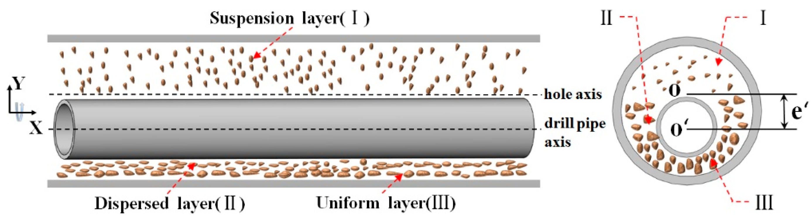
During horizontal well drilling, the downhole drill pipe is eccentric, as shown in Figure 1, where o is the center of the cross-section of the wellbore, o’ is the center of the cross-section of the drill pipe, and e’ is the eccentricity. The drill bit penetrates the rock as the drill pipe rotates and produces cuttings. Some of these are carried by the drilling fluid from the bottom of the well to the ground, while others sink under the action of gravity and friction to form a cuttings bed. A three-layer model was used to establish a numerical model of cuttings transport in horizontal small-bore wells. The uniform layer (III) is the debris layer, which has a uniform and constant cuttings concentration. Above this layer, the cuttings are dragged and lifted by the viscous fluid to the upper surface and continue to move under the action of gravity and friction in a layer called the dispersed layer (II). Above the moving bed, the cuttings are evenly distributed in the annulus in a layer known as the suspension layer (I).

The flow of drilling fluids through the annulus in this work is either laminar or low Reynolds number turbulent flow. A Euler–Euler two-phase flow model is used to study the flow behavior of the drilling fluid and the cuttings in the annulus. The model takes account of collisional interactions between cuttings particles and between these particles and the walls of the rotating pipe and the wellbore. The collisional interaction is described using the kinetic theory of granular flows with a granular temperature [32]. In this model, both the drilling fluid and cutting particles are subject to interphase forces.

During the process of drilling, cuttings transport is potentially influenced by a number of factors, including the production of gas and water at the bottom of the well in the region of the BHA (Bottom Hole Assembly), the compressibility of the drilling fluid, and changes in the temperature of the annulus [33,34,35,36]. Equipment, such as sand removers and cyclones, are located on the ground. However, we are interested in cuttings transport in horizontal sections of the annulus that are far from the BHA and in which the flow of drilling fluid is stable and has little dependence on temperature. Therefore, to avoid a huge computational workload, we make the following simplifying assumptions when constructing our CFD (Computational Fluid Dynamics) model [16,37]:

1. The influence of the annulus temperature and the production of gas and water at the bottom of the well on the flow of the drilling fluid can be neglected;

2. The drilling fluid in the flow field is incompressible;

3. There is no slip between each layer of solids and liquid;

4. The cuttings in any wellbore section are assumed to be particles of the same size and (spherical) shape.

2.1. Governing Equation

The flow of drilling fluid transporting cuttings in the wellbore can be considered as unstable fluid flow in a closed pressurized system. This will produce a water hammer in regions of the drill string joint with variable area and shape. The drilling fluid flow can be considered to be unstable, and its basic equations are those of mass and momentum conservation. The mass conservation equations for drilling fluid and cuttings, assuming a constant mechanical drilling rate and a constant drilling fluid flow rate [38,39,40], are

$${\nu }_{Ⅰf}{S}_{Ⅰ}{\rho }_f(1-C_{Ⅰ})+{\nu }_{Ⅱf}{S}_{Ⅱ}{\rho }_f(1-C_{Ⅱ})={\rho }_f{Q}_p,$$

(1)

$$m_{Ⅲ}+(S_{Ⅰ}{C}_{Ⅰ}{\nu }_{Ⅰc}{\rho }_{Ⅰ}+S_{Ⅱ}{C}_{Ⅱ}{\nu }_{Ⅱ}{}_c{\rho }_{Ⅱ})t={\rho }_c{v}_R{S}_{w}t.$$

(2)

respectively, where the mass and drilling time of the uniform layer have been considered.

The law of conservation of energy implies that the density and velocity of the drilling fluid are constant during the drilling process. The energy conservation equations of the suspension layer (I), the moving cuttings bed (the dispersed layer, II), and the stationary cuttings bed (the uniform layer, III) can then be expressed as [38,39,40]

$$(P_1-P_2)S_{Ⅰ}-{\tau }_{Ⅰ-Ⅱ}{l}_{Ⅰ-Ⅱ}L-{\tau }_{Ⅰ}{}_{-w}{l}_{Ⅰ-w}L-{\tau }_{Ⅰ-}{}_p{l}_{Ⅰ-p}L=0,$$

(3)

$$(P_1-P_2)S_{Ⅱ}+{\tau }_{Ⅰ-Ⅱ}{l}_{Ⅰ-Ⅱ}L-{\tau }_{Ⅱ}{{}_{-}}_w{l}_{Ⅱ-w}L-{\tau }_{Ⅱ-}{}_p{l}_{Ⅱ-p}L=0,$$

(4)

$$(P_1-P_2)S_{Ⅲ}+{\tau }_{Ⅱ-Ⅲ}{l}_{Ⅱ-Ⅲ}L=0.$$

(5)

respectively.

The non-Newtonian rheological properties of the drilling fluid are represented by a power law model [24]:

$${\mathsf{\tau }}_1=\eta (D)\cdot D,$$

(6)

$$D=\left(\frac{\partial v_{1j}}{\partial x_i}+\frac{\partial v_{1i}}{\partial x_j}\right),$$

(7)

$$\gamma =\sqrt{\frac{1}{2}D:D},$$

(8)

$$\eta =K{\gamma }^{n-1}.$$

(9)

The turbulent viscosity of the drilling fluid is calculated using the shear stress transfer k-ω model, where k and ω are the turbulent kinetic energy and specific dissipation rate, respectively [41]. The transport equations for k and ω are

$$\frac{\partial }{\partial t}\left({\rho }_{l}k\right)+\frac{\partial }{\partial x_i}\left({\rho }_{l}k{\mathit{v}}_{\mathrm{ll}}\right)=\frac{\partial }{\partial x_j}\left({\Gamma }_k\frac{\partial k}{\partial x_j}\right)+G_k-Y_k,$$

(10)

$$\frac{\partial }{\partial t}\left({\rho }_l\omega \right)+\frac{\partial }{\partial x_i}\left({\rho }_l\omega {\mathit{v}}_{\mathrm{ll}}\right)=\frac{\partial }{\partial x_j}\left({\Gamma }_{\omega }\frac{\partial \omega }{\partial x_j}\right)+G_{\omega }-Y_{\omega }+D_{\omega }.$$

(11)

The resistance between the two phases is calculated using the Huilin–Gidaspow model [42] to obtain the coupling momentum transfer between the drilling fluid and cutting particles, which can be expressed as follows:

$$\beta =\phi {\beta }_{\mathrm{E}}+(1-\phi ){\beta }_{\mathrm{W}\&\mathrm{Y}},$$

(12)

$$\phi =\frac{1}{2}+\frac{\arctan \left[262.5\left({\epsilon }_{\mathrm{s}}-0.2\right)\right]}{\pi },$$

(13)

$${\beta }_{\mathrm{E}}=150\frac{{\epsilon }_{\mathrm{s}}^2{\mu }_l}{{\epsilon }_1{d}_{\mathrm{s}}^2}+1.75\frac{{\epsilon }_{\mathrm{s}}{\rho }_1}{d_{\mathrm{s}}}\left|v_1-v_{\mathrm{s}}\right|,$$

(14)

$${\beta }_{\mathrm{W}\&\mathrm{Y}}=\frac{3C_d{\epsilon }_1{\epsilon }_{\mathrm{s}}{\rho }_1\left|v_1-v_{\mathrm{s}}\right|}{4d_{\mathrm{s}}}{\epsilon }_1^{-2.65}.$$

(15)

2.2. Numerical Models and Boundary Conditions

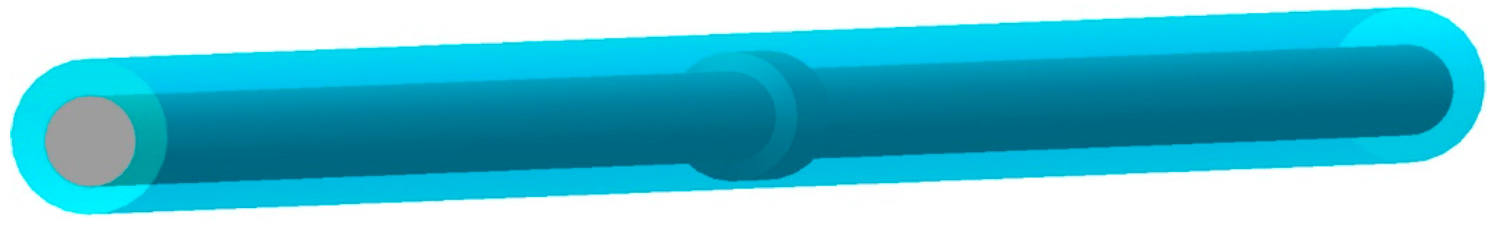
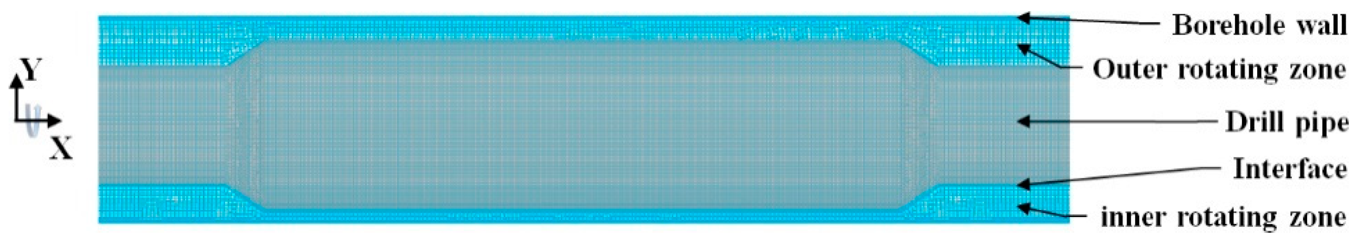
The computational domain is the annulus between the drill pipe and the borehole wall. There are assumed to be no cracks in the borehole wall. The eccentric annulus model of a six-inch (152.4 mm) wellbore in a horizontal well is illustrated in Figure 2. The model uses part of the drill string for a simulation study. There are two API drill pipes, 88.9 mm in diameter and 9 m in length, with connectors installed in the middle. The inner and outer diameters of the annulus are 88.9 mm and 152.4 mm, respectively. As shown in Figure 3, a structured hexahedral mesh is used for meshing, with the mesh near the wall is partially encrypted. The parameters used in the numerical simulation are determined by experimental measurements, as shown in

Table 1. Detailed parameters used in simulations.

Property	Simulation Value	Units
Drill pipe diameter	88.9	mm
Outside diameter of drill pipe joint	127	mm
Inner diameter of wellbore	152.4	mm
Eccentric distance	5	mm
Drill pipe rotation speed	0, 60, 120, 180	rpm
Drilling fluid density	1200	kg/m3
Particle diameter	1, 2, 3, 4, 5	mm
Particle density	2600	kg/m3
Roughness height	1, 2, 3, 4, 5	mm

. For the non-uniform surface of the borehole wall, the roughness is taken as the average diameter of cuttings on the surface.

A velocity boundary condition is adopted at the inlet, with a value equal to the pulse velocity and with the drilling fluid flow perpendicular to the boundary surface. At the outlet, a pressure boundary condition is adopted, with a value equal to the environmental pressure. For the wall boundaries, the drill pipe, etc. are assumed to be smooth without slip. The borehole wall is fixed, and the velocity satisfies a no-slip condition.

3. The Experiment of Cuttings Transport with Pulsed Drilling Fluid

3.1. Experimental Platform

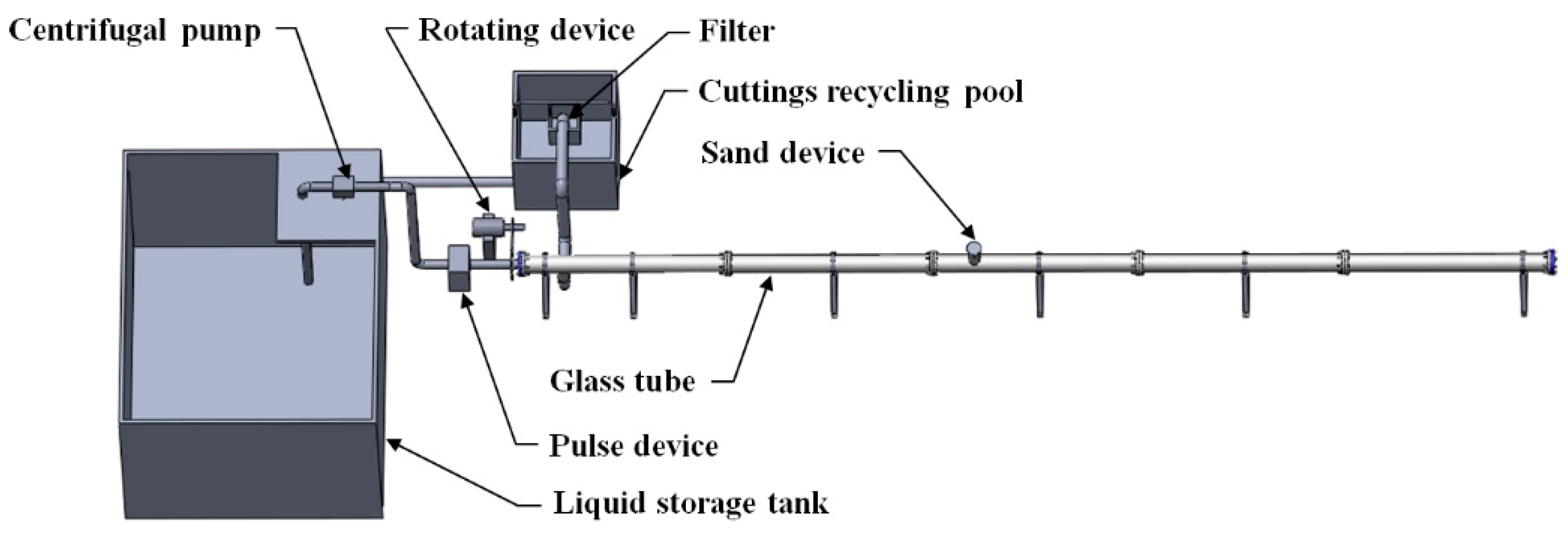
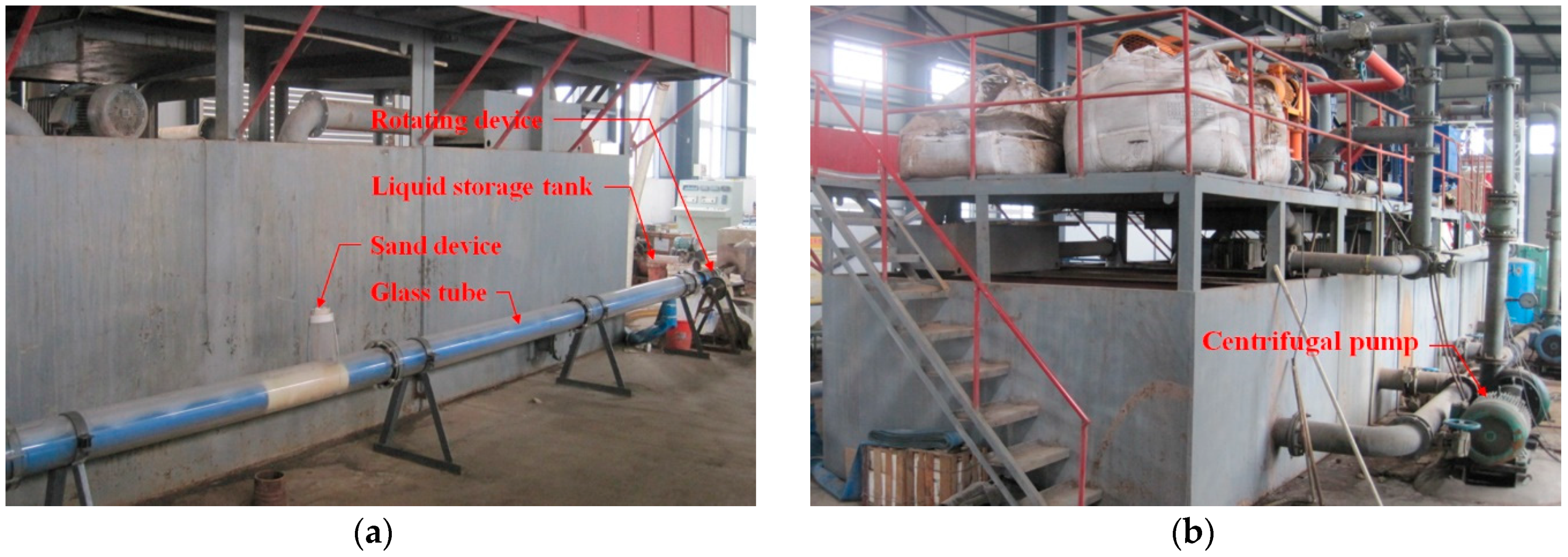
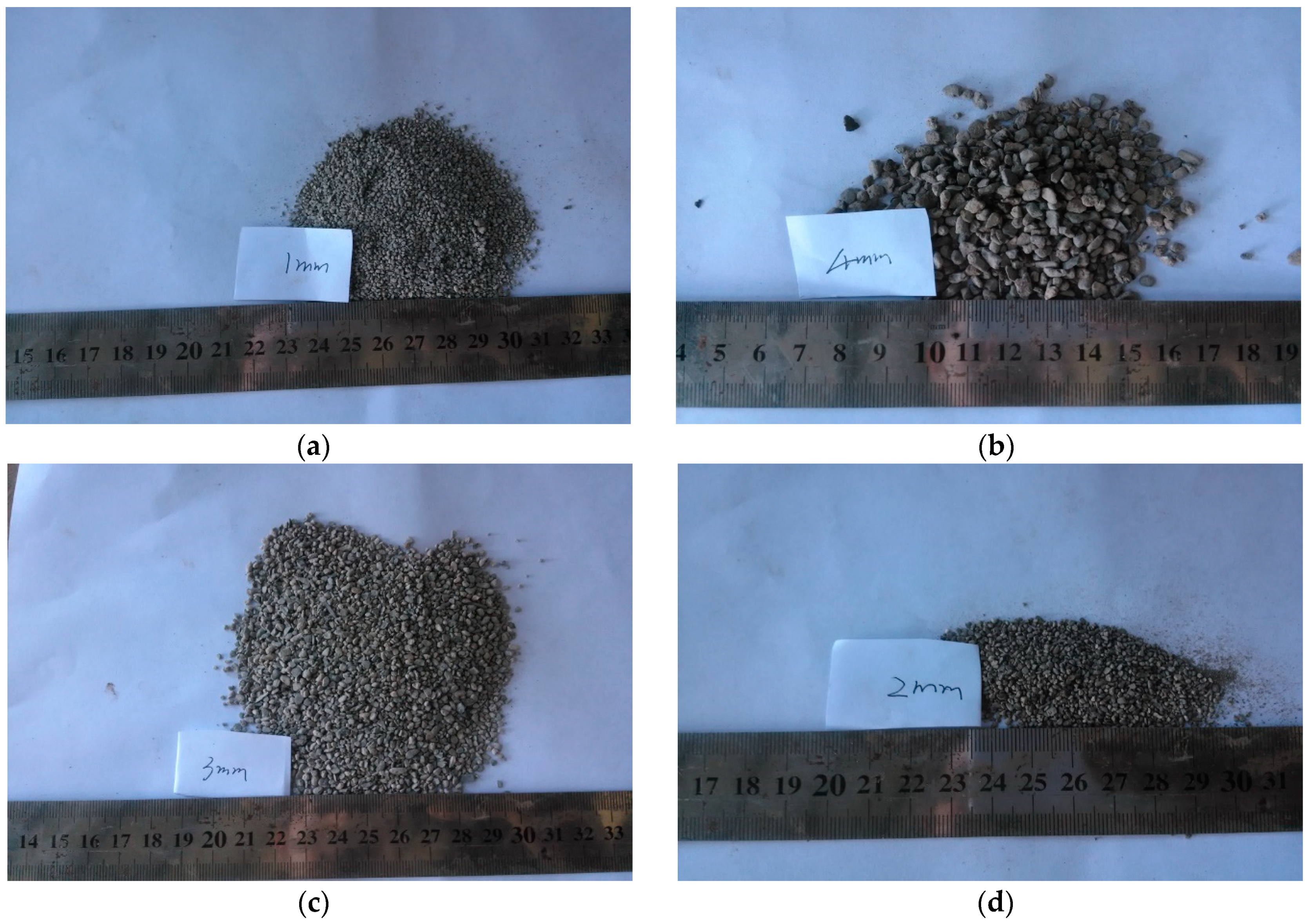
To simulate the cuttings transport process, a 1:1 visual experimental bench was constructed. The experimental set up consists principally of a Plexiglas tube, a centrifugal pump, a liquid storage tank, a sand device, a cuttings recycling pool, a filter, and a rotating device. A diagram is shown in Figure 4 and photographs in Figure 5. The total length of the Plexiglas tube is 10 m, its inner diameter is 152.4 mm, and the outer diameter of its inner tube is 88.9 mm. The experimental cuttings were collected from Well 36-3702 in Nanpu, Hebei, China, and the cuttings were classified according to their size, as shown in Figure 6. According to the experimental procedure, the pump introduces drilling fluid from the reservoir into the pipeline, thus, changing the velocity and other working conditions. A high-speed camera is used to record the transport trajectory of the cuttings, and then data, such as the time of the cuttings transport are processed and output.

The cuttings particles startup velocity is the cuttings transport velocity when cuttings start to move from rest for 0.04 s. The critical starting velocity is the velocity of the drilling fluid when the cuttings change from a static state to a moving state. The processing of cuttings transport distance data involves the conversion of video from the beginning to the end of cuttings transport into frame-by-frame images, followed by a calculation of the distance between the location of the same cuttings in the images at the beginning and the end of cuttings transport to obtain the cuttings transport distance. This process is repeated with different cuttings. The movement distances of these cuttings are then averaged, and the movement distance of the dispersed layer is finally obtained. The height data of the cuttings bed is obtained by collecting the heights of the cuttings bed in the images from the beginning to the end of the cuttings movement. The heights are then averaged, and finally, the height of the cuttings bed is obtained. The cuttings particles startup velocity is determined by using two images of cuttings, one in the static state and one in the moving state, noting the same cuttings position in the two pictures, and obtaining the movement distance of the cuttings. This is divided by time to calculate the startup velocity of the cuttings. Different cuttings are then selected, and the procedure is repeated to give the startup velocities of a large number of cuttings. These are averaged, and finally, the cuttings particles startup velocity is obtained.

3.2. Experiment Results and Discussion

The factors influencing cuttings transport include drill pipe speed, cuttings particle size, cuttings bed mass, and well wall roughness, and to study the conditions for horizontal well drilling, these parameters were varied within the experimental device. The values of the experimental parameters are listed in

Table 2. Parameters for pulsed fluid cuttings transport experiment in a horizontal well

Parameter	Simulation Value	Units
Drill pipe rotation speed	0, 30, 60, 90, 120	rpm
Cuttings size	1, 2, 3, 4, 5	mm
Cuttings bed mass	0.25, 0.5, 1, 1.5, 2	kg
Roughness height	0, 1, 3, 5	mm

. The pump displacement was 15 L/s, and the experiment continued for 8 s.

3.2.1. Stationary Cuttings Bed Destruction and Cuttings Transport Trajectory

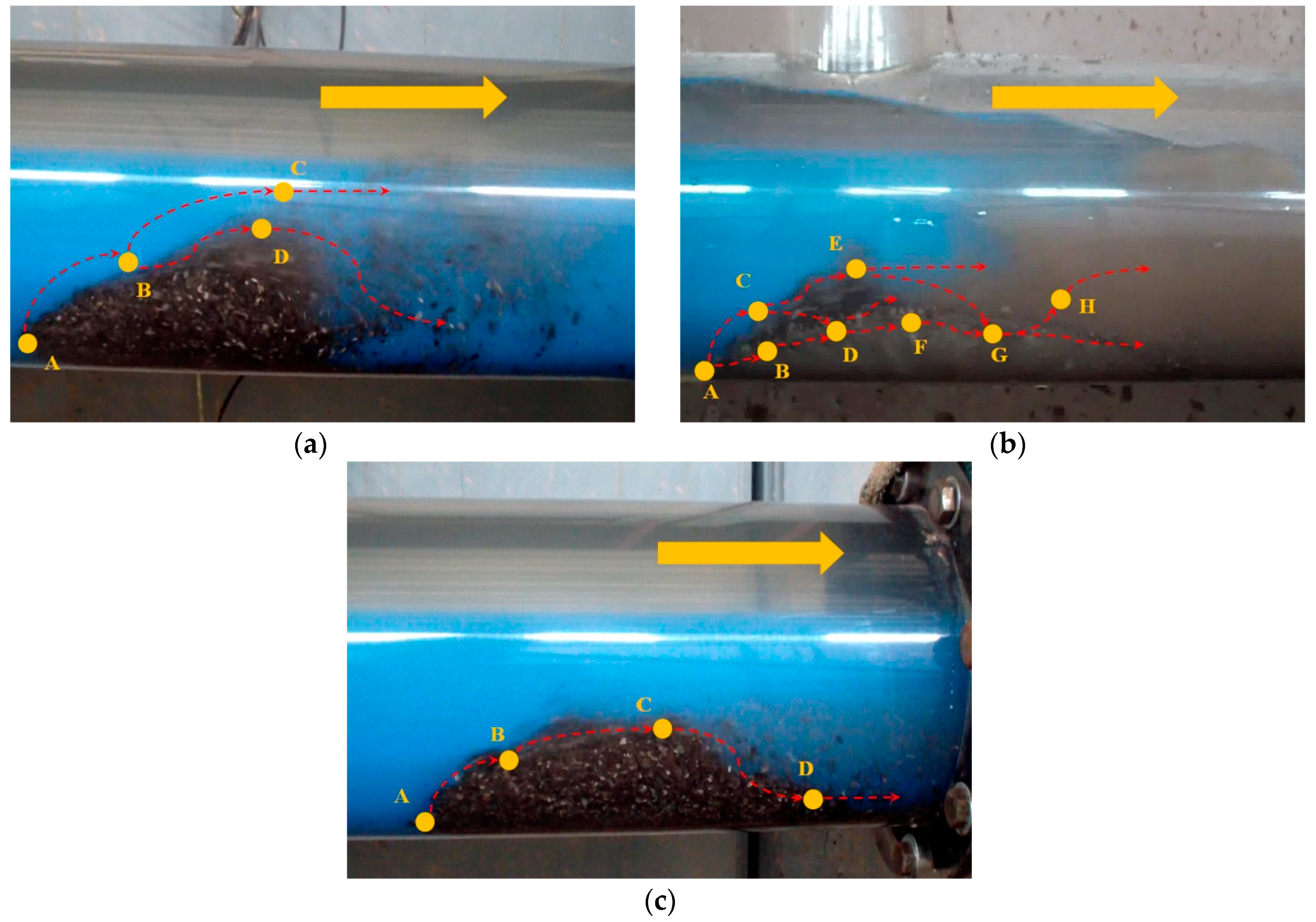
The destruction of the cuttings bed is a macroscopic process in which the drilling fluid continuously impacts the cuttings bed and leads to continuous transport and accumulation of surface particles. Experimental observations indicate that the cuttings particles are transported mainly by creep, suspension, tumbling, and hopping. It is observed that the destruction of the uniform layer by pulsed drilling fluid can be divided into three stages: Initial diffusion of the cuttings bed, suspension, and rolling of the cuttings.

The cuttings diffusion stage is shown in Figure 7a. Under the action of the drilling-fluid drag force on the windward slope of the cuttings bed, the cuttings particles start from A, contact with other surface cuttings, roll through B, and then arrive at D. They roll along the line DFG line for contact movement, and finally continue to roll at G or jump from G to H through suspension movement under the drag force. This cuttings transport trajectory is typical of large-diameter cuttings or low displacements; for other types of cuttings start from point A and then jump directly to C. When the drag force is low, the cuttings particles are deposited from C to D, before repeating the jump from D or continuing to roll to G for suspension movement. Cuttings may also start from point A and jump directly to C. When the drag force is great, they move from C to E under suspension movement. In the cuttings diffusion stage, the cuttings transport mode of pulsed drilling fluid is the same as in conventional cuttings transport, although the cuttings bed destruction is 0.5 s faster than in the conventional case.

During the cuttings suspension stage, as shown in Figure 7b, the cuttings particles start from A, jump to B, and then move from B to C under suspension movement. This is mainly a large-displacement process under a strong drilling fluid cuttings transport capacity. Another scenario is that the cuttings start from A, jump to B, and then roll from B to D, and continue to roll as the bottom particles of the cuttings bed. Compared with the conventional cuttings transport, the cuttings spend longer in this stage during the cuttings transport with pulsed drilling fluid.

During the rolling stage of the cuttings bed, as shown in Figure 7c, the suspension cuttings partially settle and begin to form a moving cuttings bed. The dispersed layer starts rolling from A to B, and then moves to C. Eventually, it rolls down to D. After D, it rolls up again and repeats the above transport trajectory. According to the experimental findings, the height of the cutting bed during the cuttings transport with pulsed drilling fluid is lower than that during conventional cuttings transport.

During the cuttings transport with pulsed drilling fluid process, the three stages of cuttings bed destruction and transport have no obvious boundaries, as in the conventional cuttings transport process. The contact transport of the cuttings is a transient process, and the trajectory has nothing to do with the trajectory in the previous cuttings phase.

3.2.2. Effect of Cuttings Size

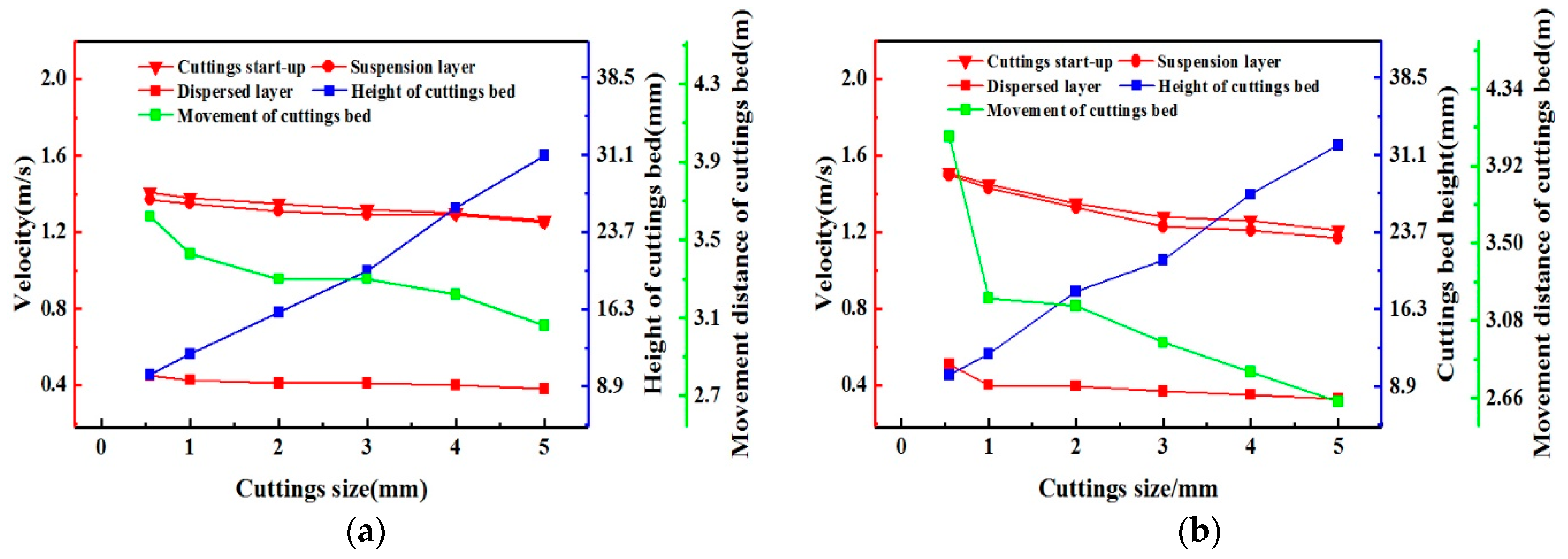
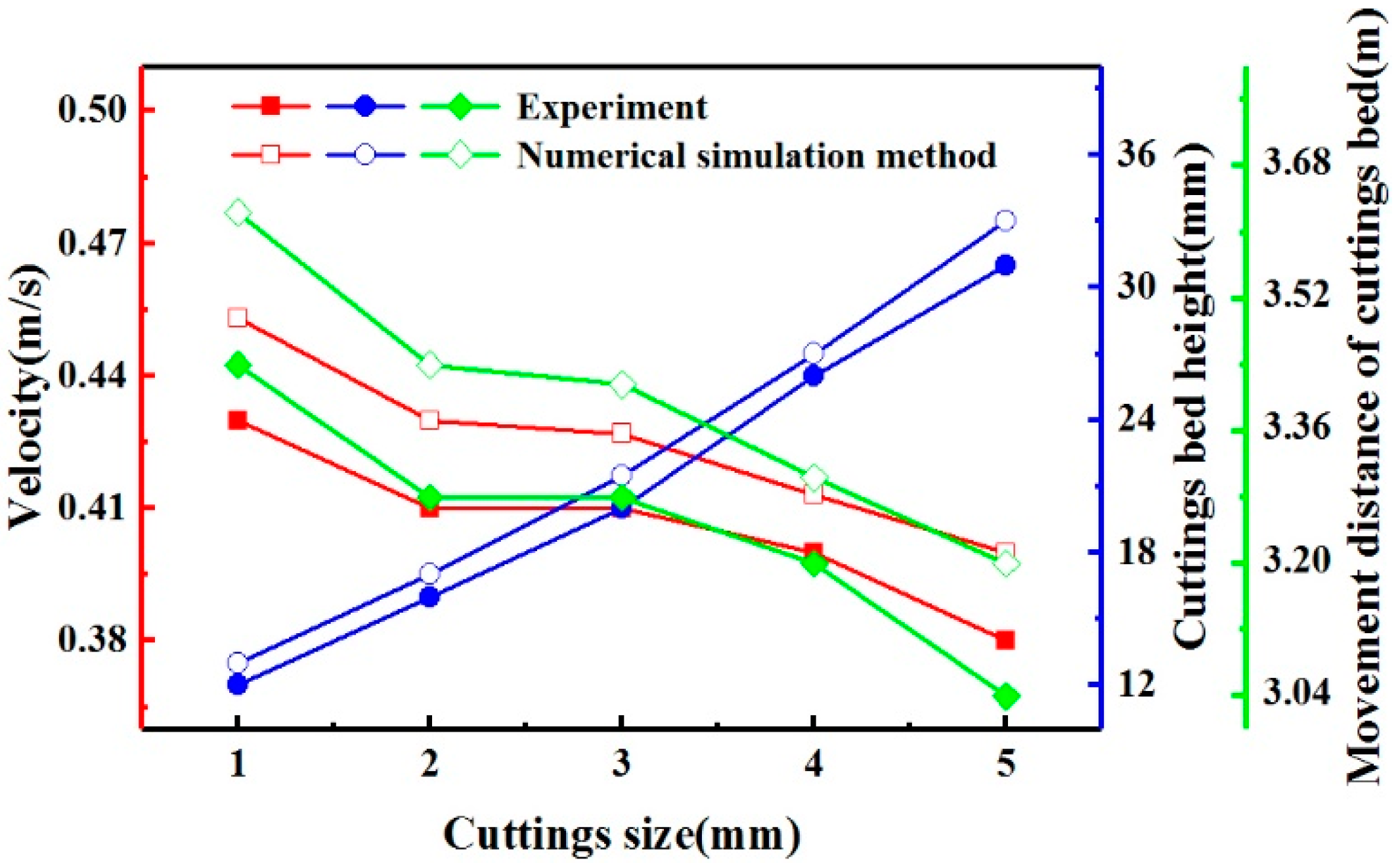
The effects of the different cuttings sizes on cutting transport are shown in Figure 8. As the cuttings’ size increases, the mass of single cuttings particles increases, and the energy required for the cuttings to move from a static state increases, i.e., the critical startup velocity increases. This decreases the particle startup velocity, the suspension cuttings velocity, and the moving bed velocity. For a cuttings diameter of 5 mm, the experimental results for pulsed fluid and conventional cuttings transport give suspension cuttings velocities of 1.25 m/s and 1.17 m/s, respectively, moving bed velocities of 0.38 m/s and 0.33 m/s, respectively, and movement distances of the cuttings bed of 3.04 m and 2.64 m, respectively. Thus, the pulsed fluid technique produces an increase of about 6.8%, 15.2%, and 15.1%, respectively. Therefore, the adoption of cuttings transport with pulsed drilling fluid gives better results. According to Figure 8, the height of the cuttings bed gradually increases. When the diameter of the cuttings is large, the clearance between them is also large, and the cuttings deposit height increases. The movement distance of the cuttings bed decreases with the increasing cuttings size. As a consequence, it is necessary to control the cuttings’ size and reduce the cuttings transport velocity. When the cuttings are less than 2 mm in diameter, the cuttings transport effect is better.

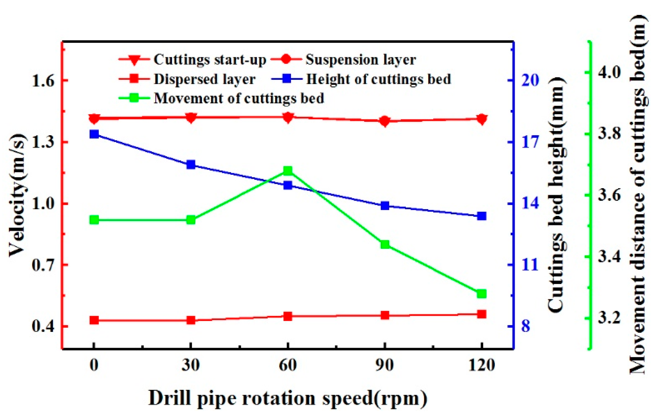
3.2.3. Effect of Drill Pipe Rotation Speed

The effects of the drill pipe rotation speed (0–120 rpm) on the mixed cuttings transport are shown in Figure 9. As the drill pipe speed increases, the cuttings startup velocity, suspension cuttings velocity, and moving bed velocity remain basically unchanged, whereas the height of the cuttings bed gradually decreases. As the drill pipe rotates, it produces more turbulence, pushing the velocity of the static cuttings in the cuttings bed up to the critical startup velocity, and thus, destroying the cuttings bed and reducing its height. This indicates that increasing the drilling speed is conducive to cuttings bed destruction. At 120 rpm, the height of the cuttings bed is 13.5 mm, which is less than the cuttings deposit critical value (10% of the annulus outside diameter). The critical value of debris accumulation is 10% of the inner diameter of the wellbore. At 60 rpm, the movement distance of the cuttings bed is 3.68 m, and at 120 rpm, it is 3.28 m. This indicates that an appropriate choice of the drill pipe rotation speed can improve the moving distance of the cuttings bed.

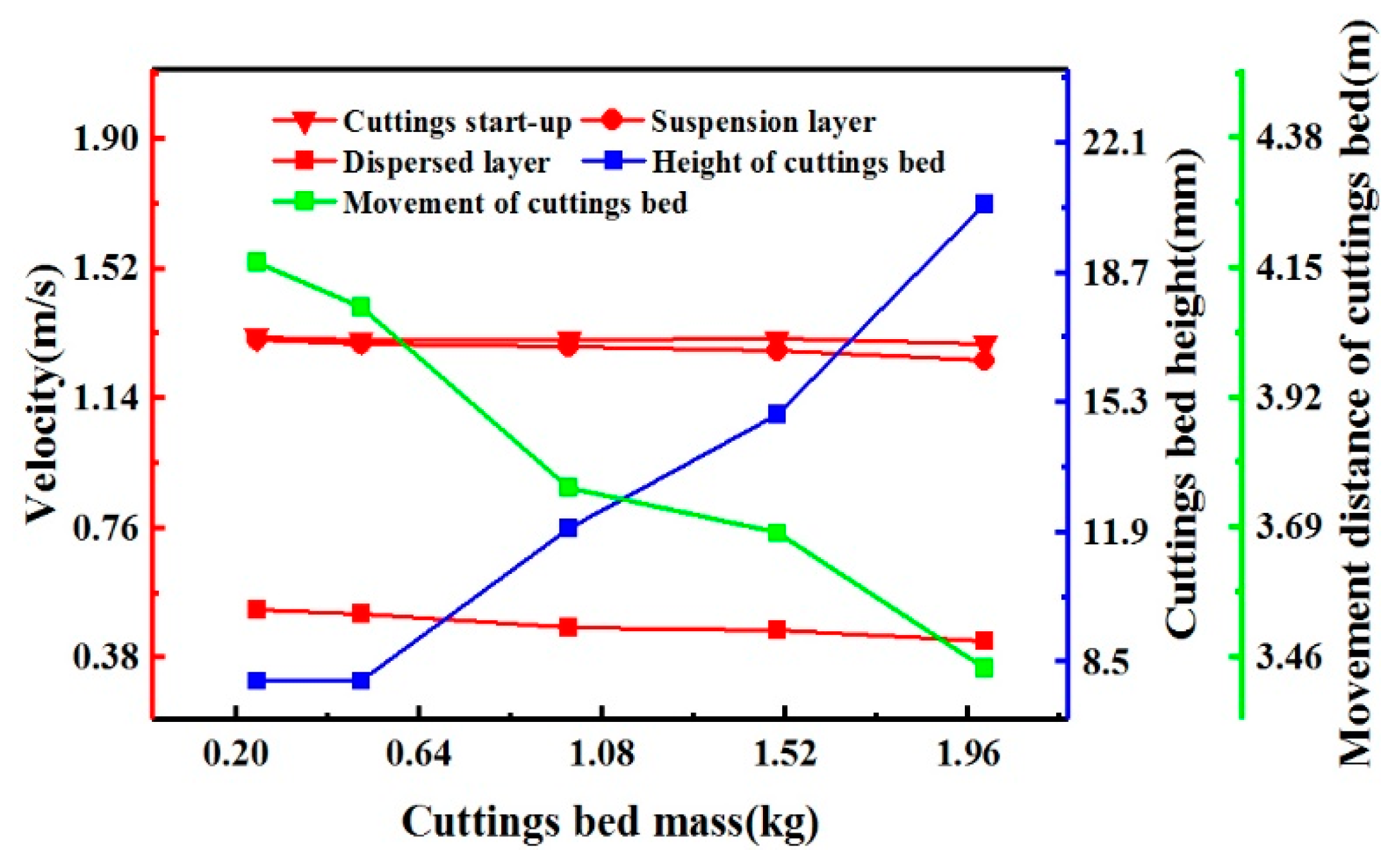
3.2.4. Effect of Cuttings Bed Mass

The effects of the cuttings bed mass (0.25–2 kg) on the transport of mixed cuttings are shown in Figure 10. As the mass of the cuttings bed increases, the total amount of cuttings to be transported per unit time increases, but the energy provided by the drilling fluid does not increase accordingly. Therefore, the velocity of the cuttings suspension gradually decreases, as does that of the moving cuttings. As the mass of the cuttings bed increases, its height increases linearly, and its movement distance decreases linearly.

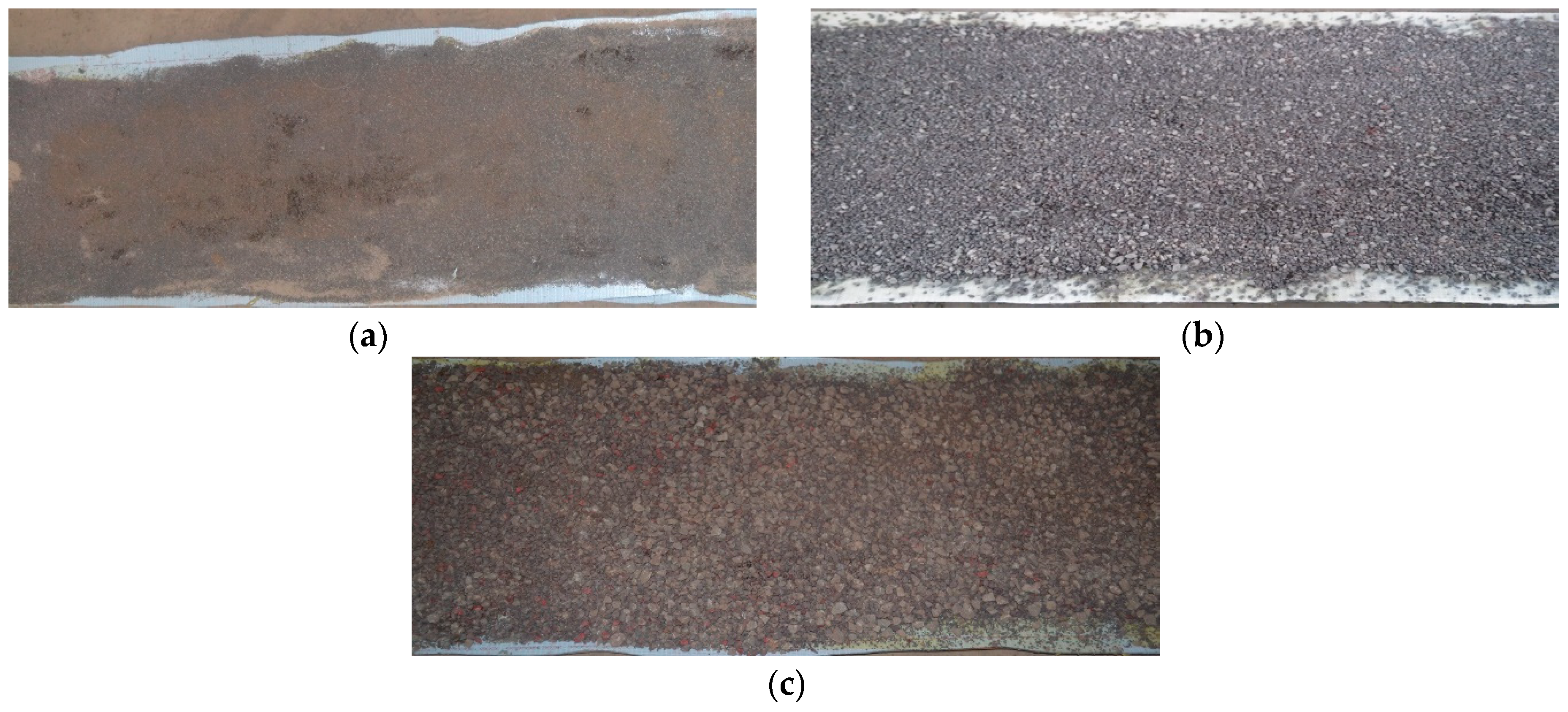
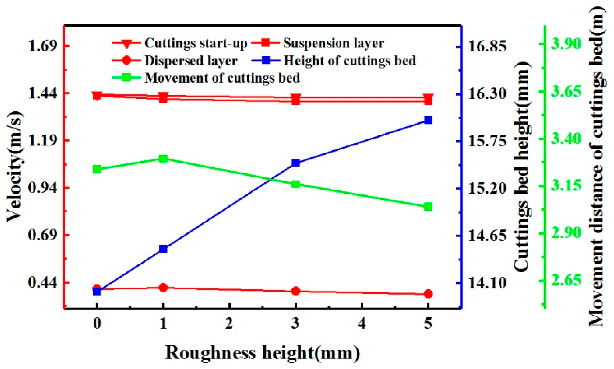
3.2.5. Effect of Roughness Height

To study the effect of roughness height on pulsed drilling fluid cuttings transport, the custom-built horizontal well wall, shown in Figure 11, was placed in the Plexiglas tube. The experimental results are shown in Figure 12. As the shaft lining roughness increases, more energy is required to start the static cuttings moving in front of the cuttings bed against static friction. Therefore, the starting speed decreases. As the shaft lining roughness increases, the height of the cuttings bed increases slightly, and the moving velocity of the cuttings bed decreases. The movement distance of the cuttings bed initially increases before decreasing. This means that increasing the shaft lining roughness is not conducive to cuttings transport. During drilling, it is, therefore, necessary to take appropriate control measures.

3.3. Sensitivity Analysis of Pulse Parameters of the Experiment

The pulse period $T$, pulse amplitude $U_m$, pulse width $t_w$, duty cycle $q$, and pulse peak $U_{\max }$ are introduced to describe the waveform of the pulsed drilling fluid velocity. The pulse period $T$ is the interval between adjacent pulses. The pulse amplitude $U_m$ is the change in the pulse velocity from minimum to maximum. The pulse width is the time interval between two points at 0.5 of the pulse leading edge and pulse trailing edge. The pulse front is the waveform of the rising part of a pulse. The back edge of a pulse is the waveform of the descending portion of a pulse. The duty cycle $q$ is the ratio of the pulse width $t_w$ to the pulse period $T$ minus the pulse width $t_w$. The pulse peak $U_{\max }$ is the maximum pulse value. The pulse amplitude ratio is the difference between the pulse peak and the pulse mean divided by the pulse mean. The proportion of the duty cycle is the ratio of the pulse width $t_w$ to the pulse period $T$ minus the pulse width $t_w$.

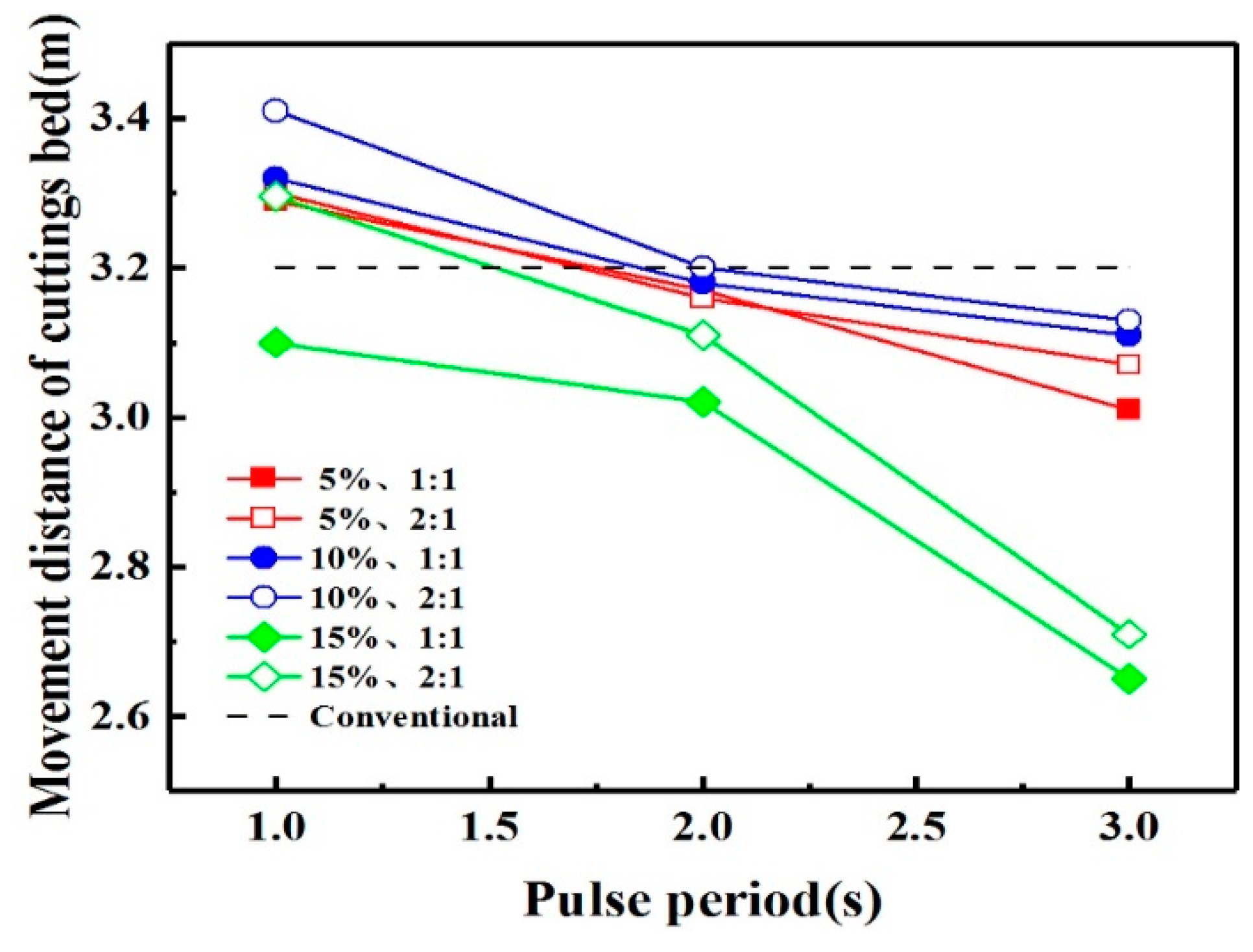
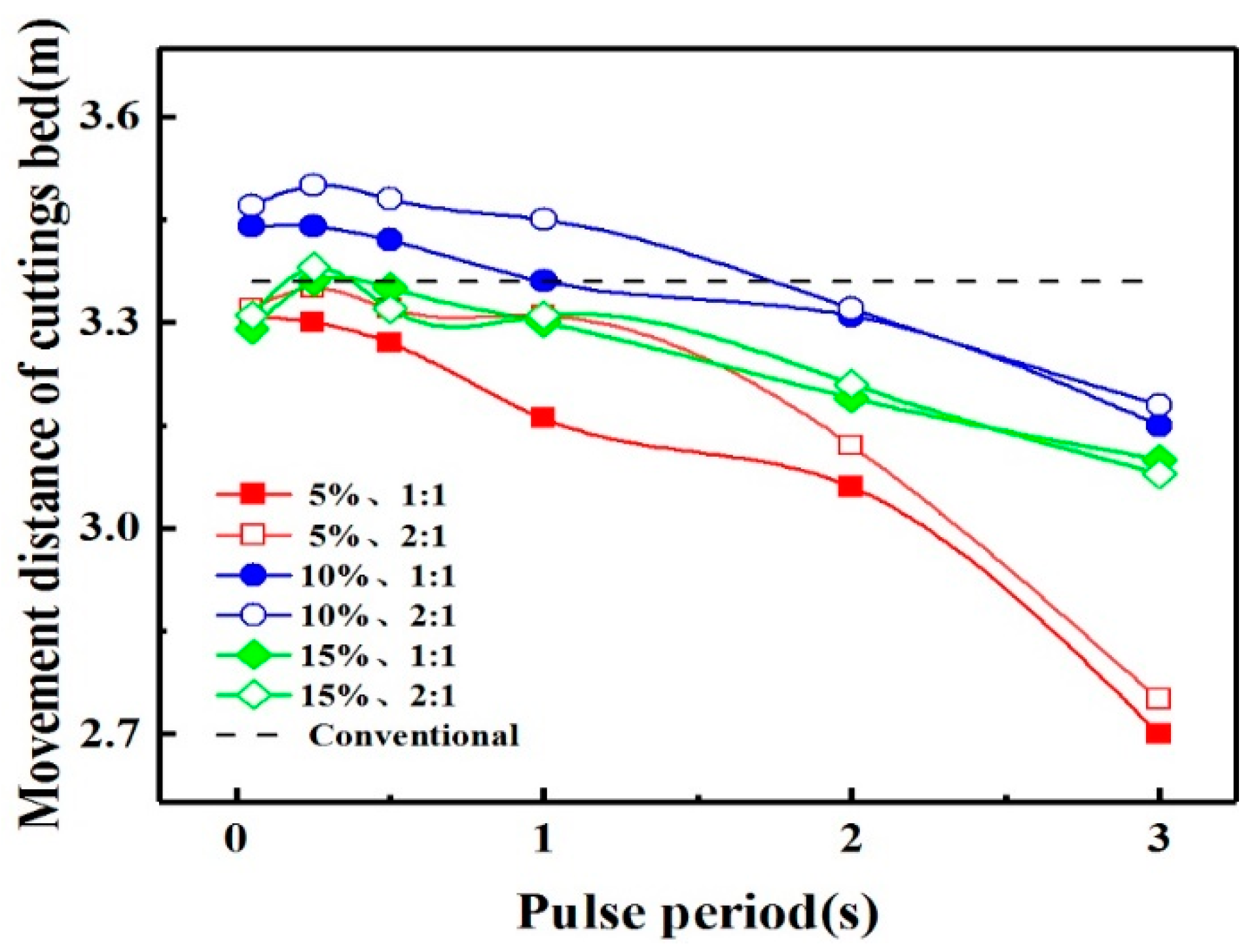
The pulse parameter range is determined by the experimental conditions. The pulse amplitude ratio was set to 0%, 5%, 10%, and 15%, and pulse periods of 1 s, 2 s, and 3 s were considered. Duty cycles of 1:1 and 2:1 were also examined. A pulse amplitude ratio of 0% is equivalent to conventional cuttings transport.

The experimental results are shown in Figure 13. With increasing pulse period, the movement distance of the cuttings bed gradually decreases, indicating that the optimal value of the pulse period is T = 1 s. At T = 1 s, a duty cycle of 2:1 and a pulse amplitude ratio of 10% gives a greater movement distance than other values of these parameters. Therefore, the optimal parameters for the experiment are a pulse period of 1 s, a pulse amplitude ratio of 10%, and a duty cycle of 2:1.

4. Numerical Simulation of Cuttings Transport with Pulsed Drilling Fluid

4.1. Numerical Model Validation

To validate the numerical model, we compare the results from a numerical simulation with the experimental results under the same conditions. The migration velocity, cutting bed height, and the moving distance of the dispersion layer are taken as evaluation parameters. As can be seen from Figure 14, the average error is 5.21%, which is acceptable for engineering requirements. The numerical model described in this paper is, therefore, suitable for investigating the behavior of cuttings transport using pulsed drilling fluid.

4.2. Numerical Simulation of Three-layer Model of Cuttings Transport with Pulsed Drilling fluid

The three-layer model considers the uniform layer, the moving cuttings bed, and the suspension cuttings bed. The initial cuttings bed is provided at the inlet. The stationary cuttings bed has a height of 10 mm, a concentration of 90%, and a length of 400 mm. The dispersed layer has a height of 10 mm, a concentration of 50%, and a length of 400 mm. The movement of the cuttings is observed for 15 s.

4.2.1. Cuttings Bed Pulse Destruction Process

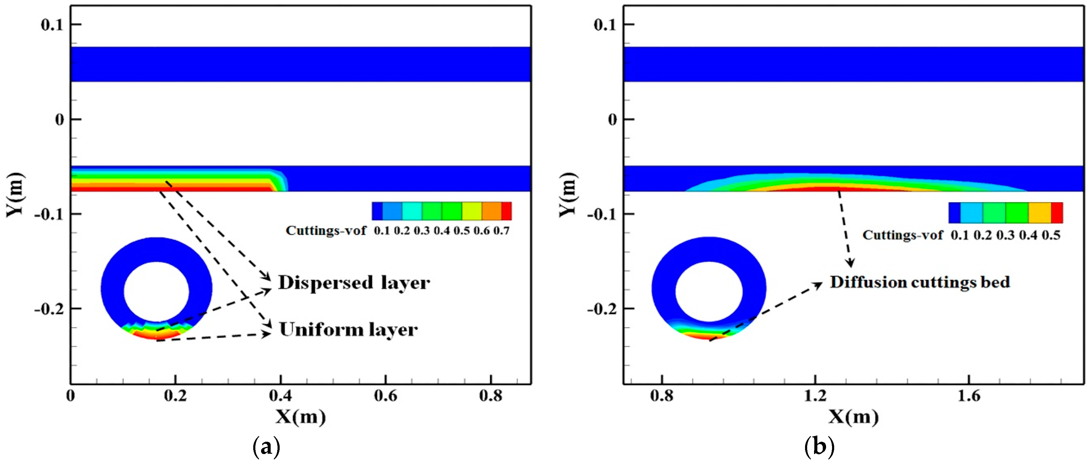
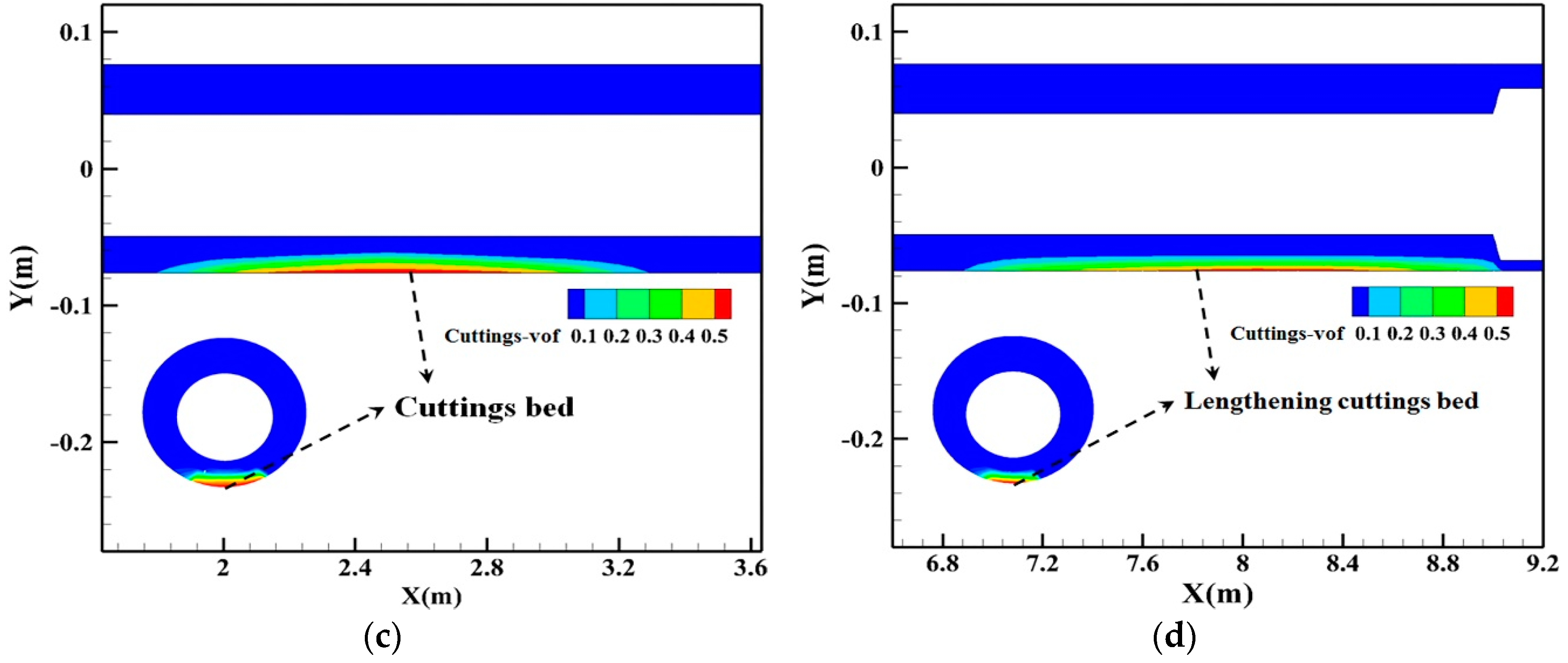
An initial cuttings bed is placed at the inlet, as shown in Figure 15a. The drilling fluid has a pulse period of 0.15 s, a pulse amplitude ratio of 12.5 %, and a duty cycle of 3:1. As shown in Figure 15b, after t = 2.5 s, the initial cuttings bed is completely diffused. At this time, the maximum volume fraction of the cuttings bed is 55%, which is 31.25% lower than the initial concentration. In Figure 15c, after t = 5 s, the cuttings bed has been transported 2.5 m under the action of the drilling fluid, and the length of the cuttings bed is 1.58 m. As shown in Figure 15d, at t = 15 s, the cuttings bed has moved to the joint. At this time, the maximum volume fraction of the cuttings bed is 55.8%, the length is 2.15 m (~5.38 times the initial length), and the movement distance of the cuttings bed is 8.18 m. According to the results of calculations for conventional cuttings transport, the time required for complete diffusion of the cuttings bed is 3 s, the movement distance of the bed is 7.38 m, and the length of the bed is 2.57 m. The use of cuttings transport with pulsed drilling fluid destroys the cuttings bed more quickly, carries the cuttings farther, and reduces the length of the cuttings bed.

4.2.2. Effect of Cuttings Size

The effects of the cuttings’ size (1–5 mm) on cuttings transport of the three-layer model are shown in Figure 16. As the cuttings’ size increases, the volume fraction of the uniform layer decreases significantly. The gap between larger cuttings is also relatively large and is filled with drilling fluid. As the volume fraction of the uniform layer becomes smaller, the height of the cuttings bed increases significantly, far exceeding the critical value (10% of the outer diameter of the annulus), which is not conducive to cuttings transport. The movement distance of the cuttings bed drops to 7.1 m at a cuttings size of 2 mm. This shows that larger cuttings sizes are not conducive to their transport. Thus, the cuttings’ size should be controlled to less than 2 mm to enhance the cuttings cleaning process.

4.2.3. Effect of Drill Pipe Rotation Speed

The effects of the drill pipe rotation speed (0–180 rpm) on cuttings transport of the three-layer model are shown in Figure 17. The rotation of the drill pipe increases the turbulence level in the drilling fluid, changing the radial transport velocity of the cuttings, and this increases the velocity of the cuttings in the cuttings bed up to the critical startup speed. The cuttings bed is, thus, destroyed through a reduction in its volume fraction. As the rotational speed of the drill pipe increases, the movement distance of the cuttings bed varies from 8.18 m (60 rpm) to 7.12 m (120 rpm). Although increasing the rotational speed is conducive to destroying the cuttings bed and reducing its height, too great a speed will change the flow field structure, producing more turbulence and inhibiting the cuttings bed transport. Therefore, the drill speed in pulsed fluid cuttings transport should be controlled to 40–70 rpm.

4.2.4. Effect of Length of Moving Cuttings Bed

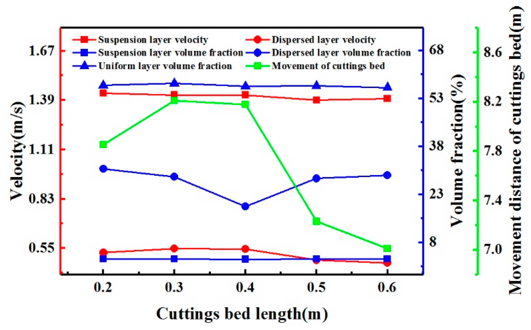
The effects of the cuttings bed length (0.2–0.6 m) on cuttings transport of the three-layer model are shown in Figure 18. As the cuttings bed length increases, the volume fraction of the cuttings bed and the velocity of the suspension cuttings show little change. The performance of pulsed fluid transport reaches a peak when the length of the cuttings bed is 0.4 m. When the length of the bed is 0.6 m, its movement distance of is 7.01 m, a decrease of 16.7% compared with the 8.18 m achieved when the length is 0.4 m. This means that increasing the length of the moving cuttings bed is not conducive to cuttings transport. The greater the length of the cuttings bed, the more difficult it is to destroy.

4.2.5. Effect of Roughness Height

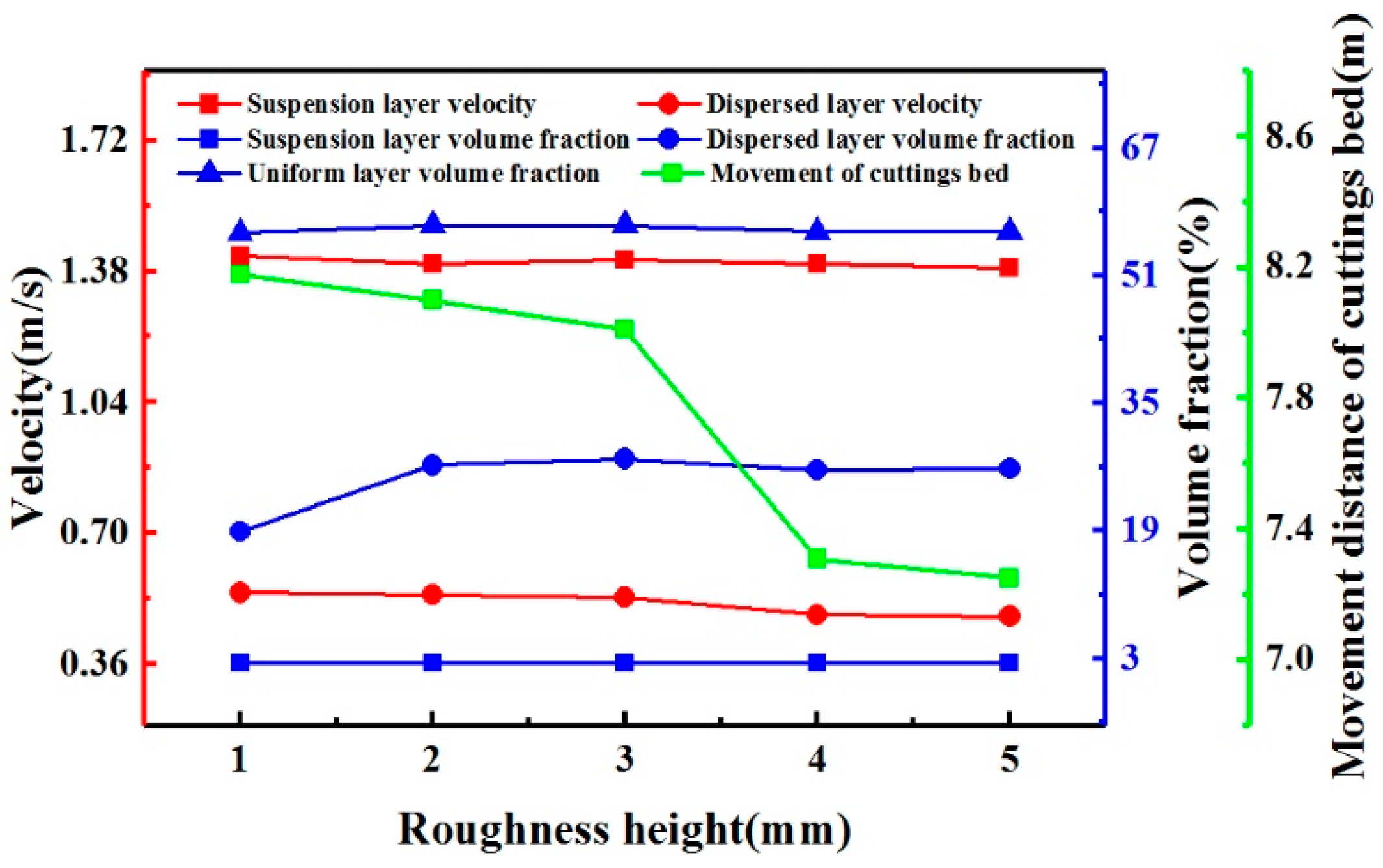
The effects of the roughness height (1–5 mm) on cuttings transport of the three-layer model are shown in Figure 19. It can be seen that an increase in roughness does not affect the volume fraction of the cuttings bed or the cuttings transport velocity. In the three-layer model, increasing the shaft lining roughness enhances the dynamic friction between the cuttings and the shaft lining, thus, increasing the resistance to cuttings transport and decreasing the cuttings transport capacity. When the roughness is 3 mm, the movement distance of the cuttings bed is 8.01 m. A roughness of 4 mm reduces the movement distance to 7.3 m. This indicates that the shaft lining roughness has a strong influence on cuttings transport and should be controlled to less than 3.2 mm.

4.3. Pulse Parameter Sensitivity Analysis

Due to experimental conditions, the parameters of cuttings transport with pulsed drilling fluid have yet to be verified. Reduce the range of pulse parameters obtained from the experiment and continue to calculate, as shown in Figure 20. According to the figure, cuttings transport effect is better than that of 1s when the pulse period T is 0.05s, 0.25s and 0.5s. It can be seen that the T=1s obtained by the experiment is not the optimal period of the pulse-carrying rock. When the pulse amplitude ratio is 5% and 15%, the movement distance of cuttings transport is less than 10%. When the duty ratio is 2:1, the movement distance of cuttings transport is longer than that at 1:1. Therefore, the optimal pulse-carrying parameters need to be further calculated and determined.

According to the shunt relay mechanism, the energy distribution ratio for pulsed fluid cuttings transport ranges from 0% to 15% under a pump displacement of 15 L/s, where 0% is equivalent to the conventional cuttings transport mode. The pulse frequency range is 4–50 Hz, i.e., the period of the pulse energy is 0.02–0.25 s. The duty cycle ranges from 0.5 to 0.8, as determined by the rotational characteristics of cuttings transport tools [43] and the water pulse generator [44]. The duty cycle is set to 1:1, 2:1, 3:1, or 4:1.

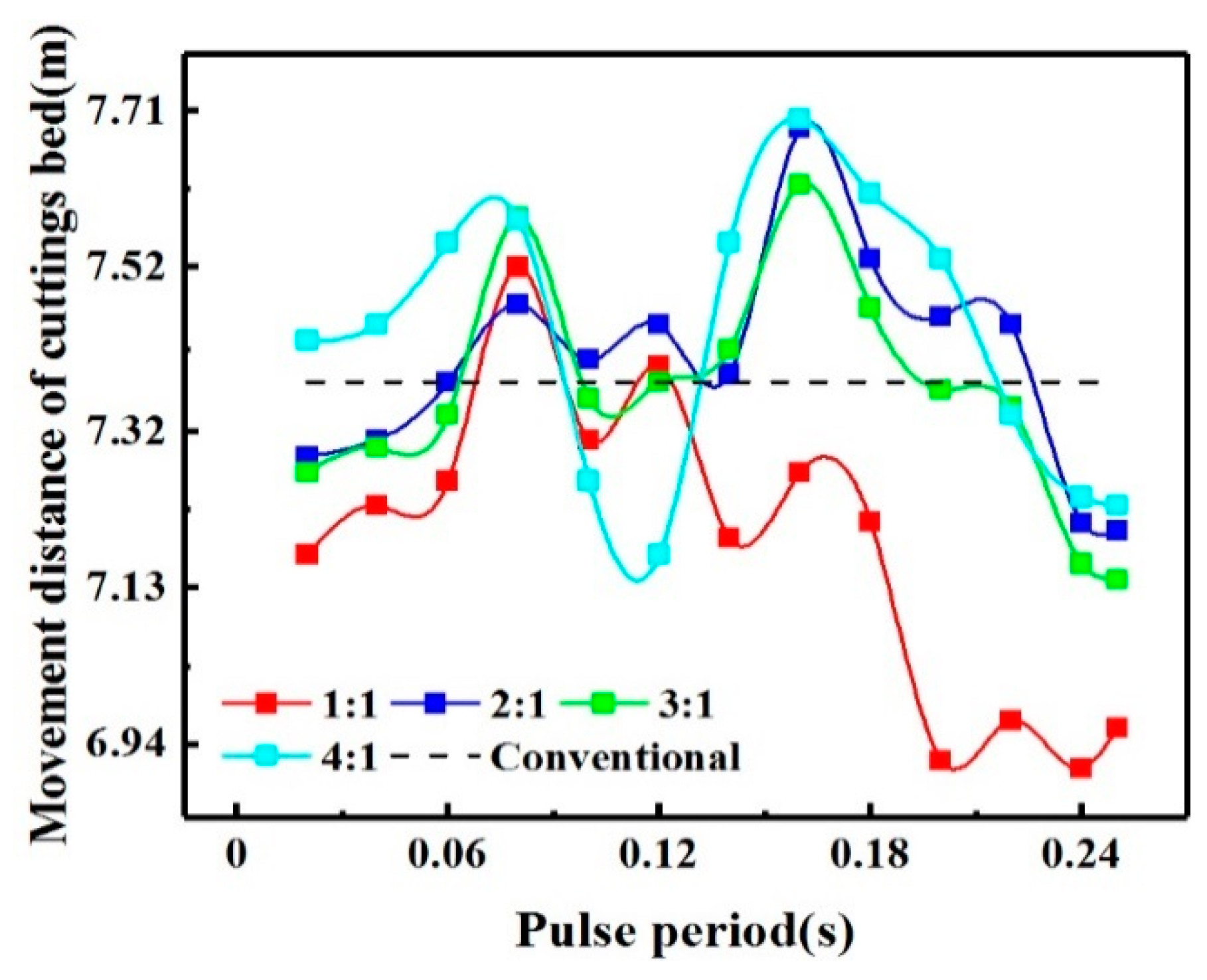
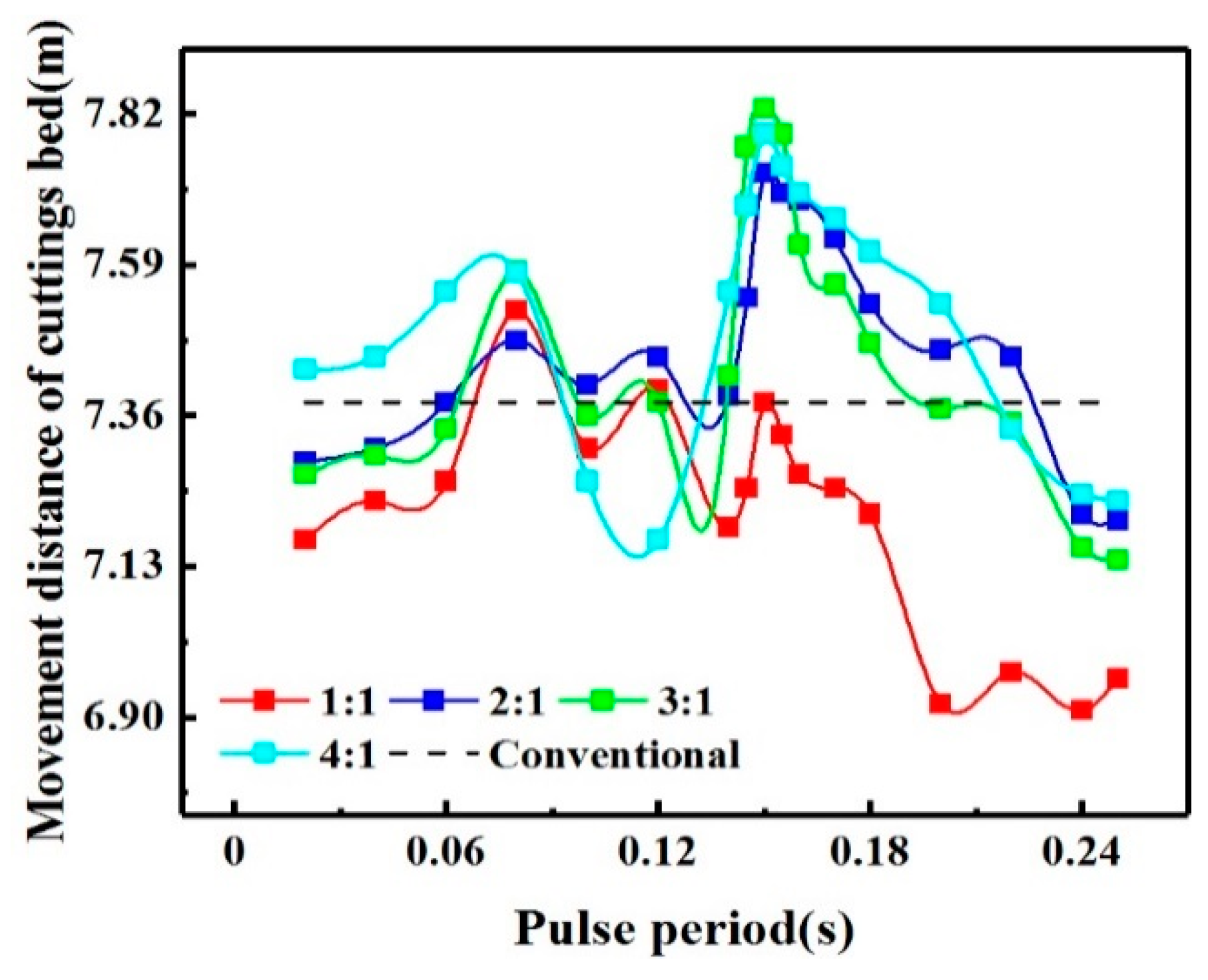
We first examine the cycle in the interval 0.02–0.25 s, starting from 0.02 s and examining cycle points at intervals of 0.02 s. The pulse amplitude ratio is taken as 10%, and the duty cycle is set to one of 1:1, 2:1, 3:1, or 4:1. Using the three-layer model, the observation time is 15 s, and the evaluation criteria are the movement distance and velocity of the cuttings bed. The initial cuttings bed in the numerical simulation has a length of 0.4 m, a height of 15.24 mm, a concentration of 90%, and a cuttings size of 1 mm, and the eccentricity and speed of the drill pipe are 0.16 and 60 rpm, respectively. The calculation results are shown in Figure 21. The black dashed line is the movement distance of the cuttings bed in the three-layer model. The movement distance is greatest in the interval from 0.14 s to 0.18 s. Thus, the period was refined within this interval.

The calculation results for the period interval refinement are shown in Figure 22. A pulse period of 0.15 s and duty cycle of 3:1 produce the greatest movement distance of the cuttings bed. Therefore, T = 0.15 s is the optimal cycle.

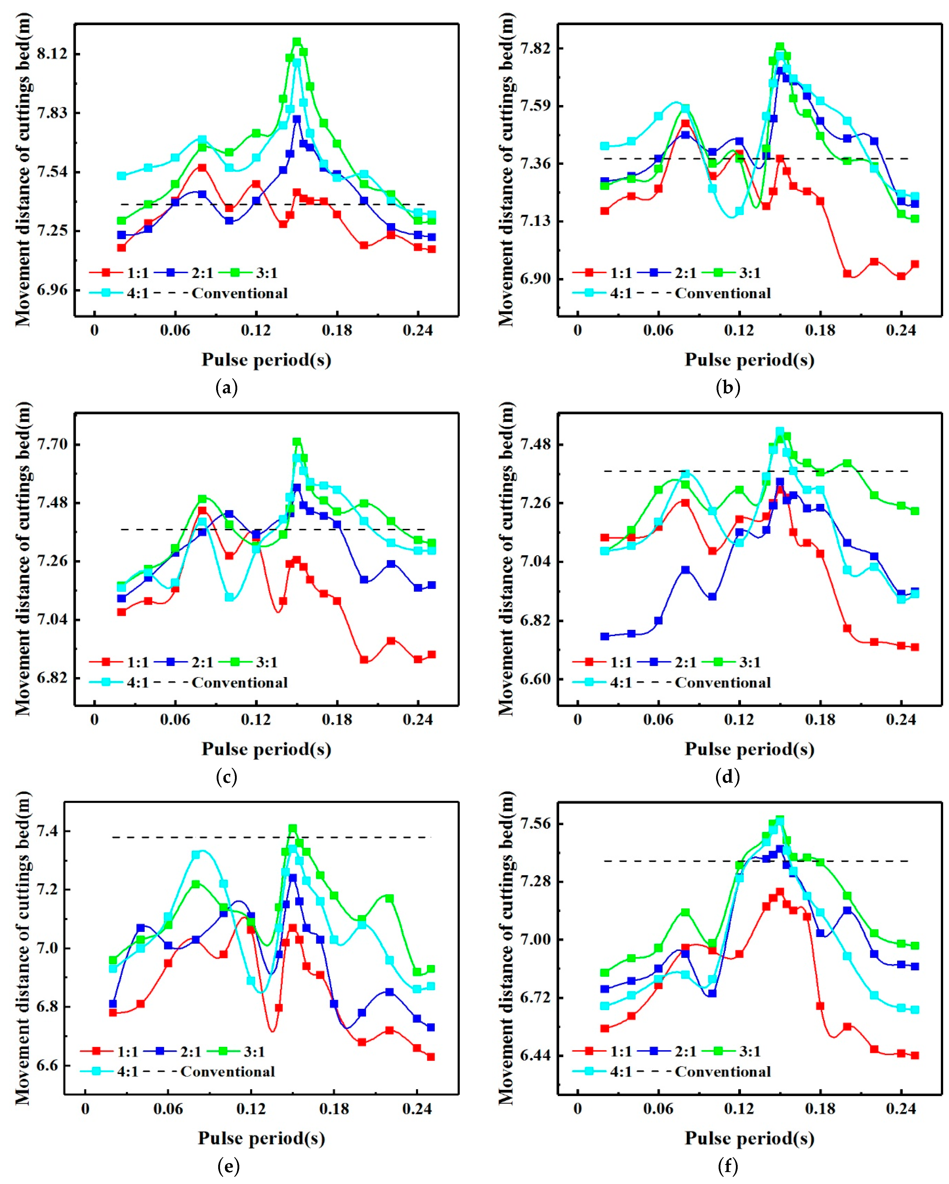
To verify that T = 0.15 s is the best period, various pulse amplitude ratios were considered, as shown in Figure 23. Under different pulse amplitude ratios, the movement distance of the cuttings bed for each duty cycle exhibits the same characteristics for different pulse periods. When the proportion of the duty cycle is 1:1, the movement distance of the cuttings bed gradually increases with the pulse period. For periods of T = 0.08 s, T = 0.12 s, T = 0.15 s, the peak state is achieved. The movement distance then gradually decreases. When comparing the movement distance of the cuttings bed at these three points, there is some variation under different pulse amplitude ratios. Most of them do not exceed the movement distance of the conventional cuttings transport bed (7.38 m). The cuttings bed movement effect with a duty cycle proportion of 1:1 is not as good as that with other ratios. When the proportion of the duty cycle is 3:1 or 4:1, the movement distance of the cuttings bed increases with the pulse period. It reaches a first peak at T = 0.08 s, and then decreases rapidly, arriving at a minimum at T = 0.1 s or T = 0.12 s. The movement distance remains unchanged for some time, and then increases to a maximum at T = 0.15 s. When comparing duty cycles, the greatest movement distance of the cuttings bed occurs with a duty cycle proportion of 3:1. Therefore, a duty cycle proportion of 3:1 is chosen as the optimal value.

According to Figure 23, when the duty cycle is 3:1, and the pulse amplitude ratio is 2.5%, the movement distance of the cuttings bed does not exceed that for conventional transport; at pulse amplitude ratios of 5% and 15%, the movement distance is only greater than that with conventional cuttings transport at duty cycles of 3:1 and 4:1; when the pulse amplitude ratios are 7.5%, 10%, and 12.5%, cuttings transport with pulsed drilling fluid is more effective than conventional cuttings transport. A ratio of 12.5% produces the greatest movement distance of the cuttings bed. Under this condition, the movement distance is 8.18 m for a period of 0.15 s, which an increase of 10.84% compared with the 7.38 m for conventional cuttings transport.

The above analysis indicates that the optimal parameters for pulsed fluid cuttings transport are a pulse period of T = 0.15 s, duty cycle of 3:1, and a pulse amplitude ratio of 12.5%. Under these conditions, the movement distance of the cuttings bed is 8.18 m, and the movement velocity is 0.545 m/s.

5. Conclusions

This paper has described a method for effectively destroying the cuttings bed and enhancing the velocity of the cuttings. A three-layer numerical simulation model of cuttings transport in horizontal small-bore wells was used to study the transport characteristics of pulsed drilling fluid driving cuttings in horizontal sections.

The experimental results show that the movement of the cuttings involves mainly creep, suspension, rolling, and leaping. According to these types of movement, the destruction of the uniform layer by pulsed drilling fluid can be divided into three stages: Initial diffusion of the cuttings bed, suspension, and rolling of the cuttings. Compared with the use of a conventional flow of drilling fluid, the cuttings are transported several times under the action of the pulsed fluid. An appropriate rotational speed helps to destroy the cuttings bed. Small cuttings produced at the drill bit reduce the height of the cuttings bed, and smaller cuttings result in a higher cuttings transport speed. Additionally, a smooth wellbore allows the cuttings to migrate further.

Cuttings transport in horizontal sections of small-bore holes is affected by the displacement of the drilling fluid. When the displacement is less than a critical value of 6.38 L/s, the cuttings remain at rest. When the pulsed drilling fluid displacement is equal to the critical displacement, the cuttings begin to be transported. In this case, the cuttings transport speed reaches 0.66 m/s after 0.04 s.

Numerical simulations indicate that the pulse parameters can directly influence cuttings transport. A pulse period of T = 0.15 s, a duty cycle of 3:1, and a pulse amplitude ratio of 12.5% produce the most effective cuttings transport. Only 2.5 s is required for the pulsed drilling fluid to destroy a fixed cuttings bed.