Application of Dipole Array Acoustic Logging in the Evaluation of Shale Gas Reservoirs

Abstract

In order to effectively evaluate shale gas reservoirs with low porosity, extra-low permeability, and no natural productivity, dipole array acoustic logging, which can provide various types of information including P-wave slowness (DTC) and S-wave slowness (DTS), is widely used. As the dipole array acoustic logging tool has a larger investigation depth and is suitable for complex borehole environments, such as those with a high wellbore temperature, high drilling fluid column pressure, or irregular borehole wall, it has been mainly applied to the evaluation of lithology, gas potential, fractures, and stimulation potential in shale gas reservoirs. The findings from a case study of the Sichuan Basin in China reveal that the acoustic slowness, S-P wave slowness ratio (RMSC), and S-wave anisotropy of the dipole array acoustic logging can be used to qualitatively identify reservoir lithology, gas potential, and fractures. Using the relationship between DTC and the total porosity of shale gas reservoirs, and combined with the compensated neutron (CNL) and shale content (V_sh) of the reservoir, a mathematical model for accurately calculating the total porosity of the shale gas reservoir can be established. By using the relationship between the RMSC and gas saturation in shale gas reservoirs and tied with density log (DEN), a mathematical model of gas saturation can be established, and the determination of gas saturation by the non-resistivity method can be achieved, delivering a solution to the issue that the electric model is not applicable under low resistivity conditions. The DTS, DTC, and DEN of shale can be used to calculate rock mechanic parameters such as the Poisson’s ratio (POIS) and Young’s modulus (YMOD), which can be used to evaluate the shale stimulation potential.

1. Introduction

Unconventional oil and gas resources, including shale gas, are very richly concentrated around the world [1]. In recent years, the production of shale oil and gas in North America has increased rapidly, which has made the exploration and development of shale gas around the world, including in China, more popular [2,3,4]. Because of the “in-situ” hydrocarbon pooling pattern of shale gas reservoirs [5,6,7], the identification of conventional reservoirs, inclusive of sandstone reservoirs, fluid property identification methods, and evaluation criteria are not fully applicable to shale gas reservoir evaluation. In addition, shale gas reservoirs have the characteristics of low porosity, extremely low permeability, and no natural productivity, so shale development requires large-scale hydraulic fracturing. Therefore, evaluation of the stimulation potential in reservoirs is an important part of shale gas reservoir evaluation and is also different from conventional oil and gas reservoir evaluation.

Currently, the use of dipole array acoustic logging to evaluate shale gas reservoirs is one of the key study topics for logging researchers [8,9]. In order to effectively evaluate the shale gas reservoirs, logging researchers have studied micro-resistivity scanning imaging logging, well circumferential acoustic imaging logging, dipole array acoustic logging, and other methods, which can be used as visual ways to exhibit development intervals in shale gas reservoirs. Among them, dipole array acoustic logging uses a larger investigation depth. The lateral investigation depth can be up to 6 m, which is more than twice that used in conventional acoustic logging, with a temperature resistance of up to 260 °C and a pressure resistance of up to 207 MPa. This type of logging is suitable for complex wellbore environments such as those with a high wellbore temperature and high drilling fluid column pressure [10]. These remarkable characteristics make it widely valued.

Previous findings revealed that there are many factors to consider in shale gas reservoir evaluation, and it is difficult to cover all aspects [11,12]. From the prospective of shale gas dipole array acoustic logging, rapid and efficient evaluation of shale gas reservoirs should be carried out in terms of lithology, fractures, gas potential, and stimulation. Previous studies and experiments have proved that reservoir fractures can cause significant changes in S-wave anisotropy, which are proportional to the strength of fractures [13,14,15]. Dipole array acoustic logging can be employed to measure S-wave anisotropy. Therefore, we studied the methods and features of dipole array acoustic logging in detail and applied them to the qualitative identification of the lithology, gas potential, and fracture effectiveness of shale gas reservoirs and the quantitative evaluation of the porosity, saturation, and reservoir stimulation potential. The cases for the typical shale gas wells of the Sichuan Basin in China are presented for analysis.

2. Evaluation Methods

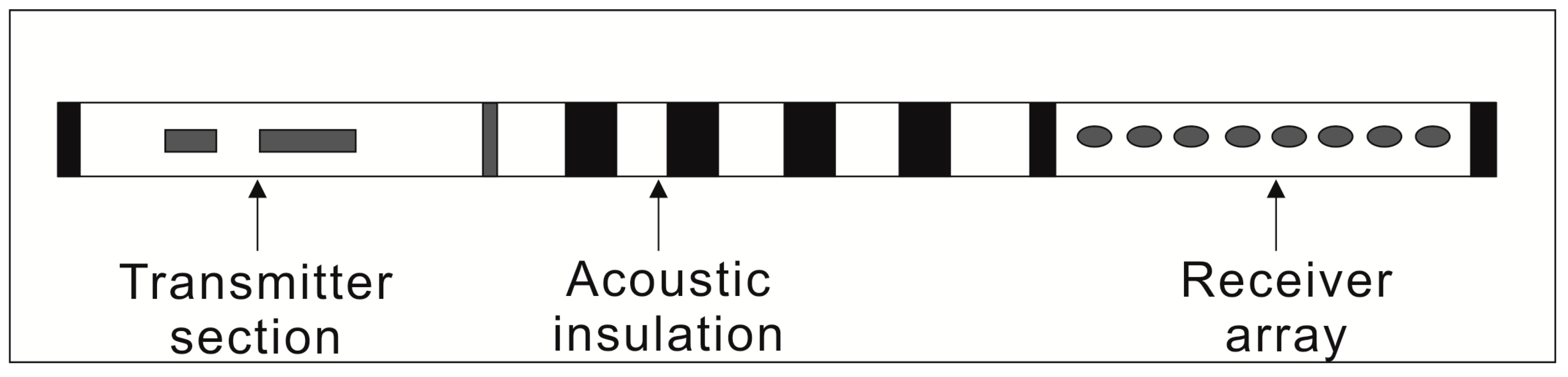
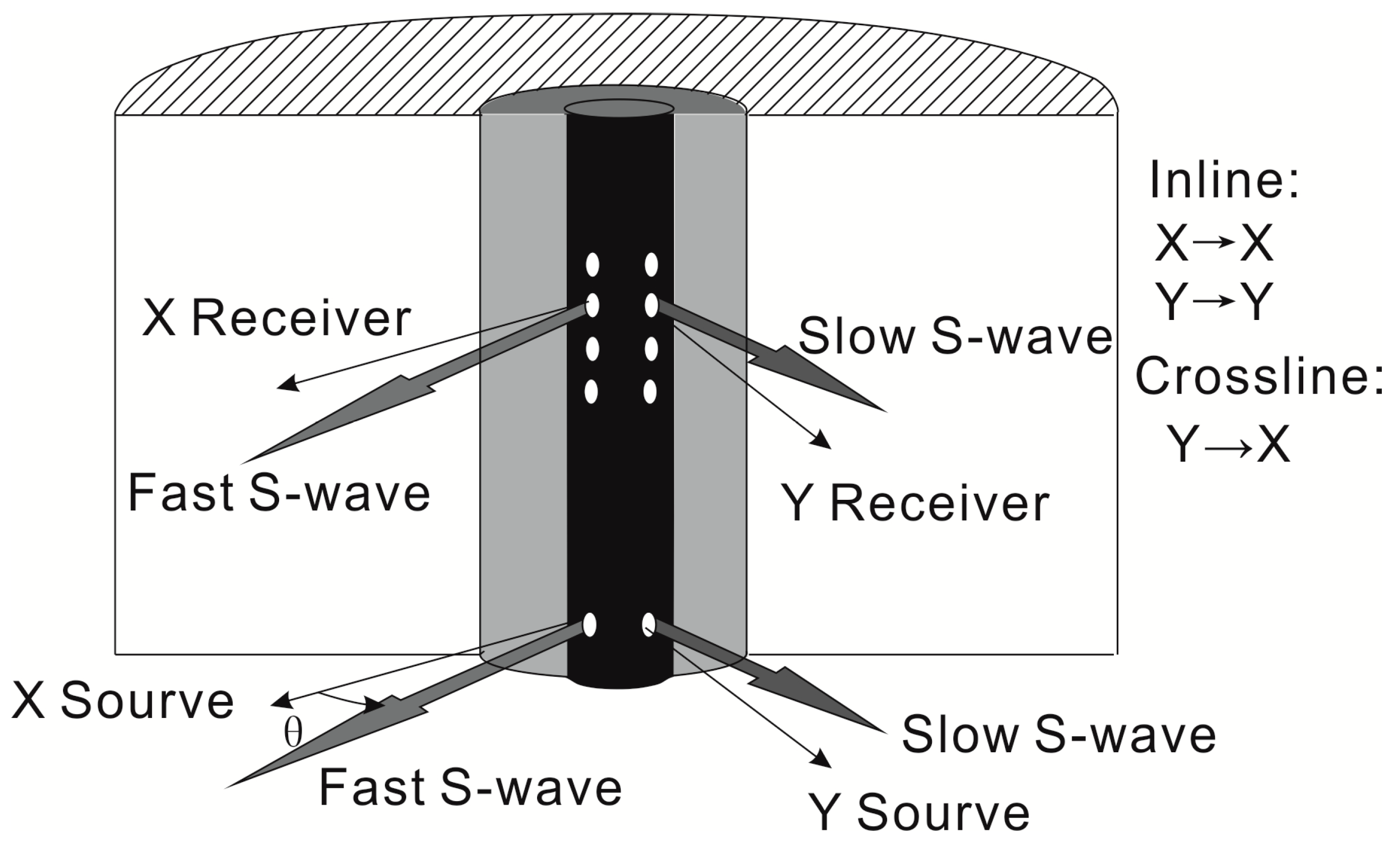
2.1. Introduction to the Tool

A dipole array acoustic logging tool usually consists of three parts: the acoustic system, the primary electronic circuit, and transmission control. Among them, the acoustic system is mainly composed of a transmitter, acoustic insulation, and a receiver array (Figure 1). The transmitter can also be a monopole transmitter or a dipole transmitter. In order to perform cross-dipole logging, the receiver array is designed to be arranged in a vertical or parallel position with respect to the dipole transmitter array direction. This type of logging tool not only measures the P-wave, S-wave, and Stoneley wave of the formation, but also applies inversion of the formation anisotropy through the cross-dipole measurement data [15,16,17,18].

2.2. Identification of Lithologies and Gas Potential

2.2.1. Identification of Lithologies

The S-P wave slowness ratio is called the RMSC or Δt_s/c and is also known as the P-S wave velocity ratio. It is closely associated with lithologies and can be employed to identify lithologies, especially the main sedimentary rocks such as shale, sandstone, and carbonate (limestone and dolomite). In the fairly tight shale zones, P-wave slowness (DTC) and S-wave slowness (DTS), which are extracted by the dipole array acoustic logging, are of higher quality than in the loose zones. Therefore, the reliable P-wave velocity and S-wave velocity can be measured in the tight heterogeneous shale zones, and the RMSC or Δt_s/c of the different lithologies and minerals has a significant difference when there is no gas in the zone (

Table 1. The S-P wave slowness ratios (RMSCs) for the main lithologies and minerals [15,19,20,21,22].

Lithologies and Minerals	P-Wave Slowness (μs·ft−1)	S-Wave Slowness (μs·ft−1)	RMSC
Shale	80.0	160–180	1.90–2.25
Sandstone	55.5	88.8–95	1.58–1.80
Limestone	47.5	88.7	1.90
Dolomite	43.5	78.3	1.80
Salt rock	67	116	1.73
Anhydrite	50	97.5	1.95
Pyrite	38	59	1.55

). The RMSC equation is as follows (Equation (1)):

$$RMSC=\frac{DTS}{DTC},$$

(1)

where DTC is the P-wave slowness of a reservoir rock, μs/ft; DTS is the S-wave slowness of a reservoir rock, μs/ft; and RMSC is the S-P wave slowness ratio of a reservoir rock, dimensionless.

In general, the RMSC is more than 2.00 for shale, 1.90 for limestone, 1.80 for dolomite, and 1.58–1.80 for sandstone, without gas in the formation [15,19,20,21]. The RMSC of shale is obviously larger than that of carbonate, and the RMSC of carbonate is obviously larger than that of sandstone. The RMSC of the water-bearing sandstone increases as the porosity and clay content increase in addition to decreases in compaction and effective stress.

2.2.2. Identification of Gas Potential

The gas potential properties of tight carbonate and shale reservoirs can be effectively identified by using the RMSC [23,24,25]. When the formation contains gas, with its temperature, pressure, and burial depth being the same or similar, both its bulk density and bulk modulus become smaller, and the shear modulus remains almost unchanged, resulting in a significant decrease in the P-wave velocity and a slight decrease or nearly no variation in the S-wave velocity. This enables the P-S wave velocity ratio, that is, the RMSC, to be greatly reduced [26].

Under the condition of a known reservoir lithology, the gas potential of the reservoir can be identified qualitatively by using the logging characteristics of smaller RMSCs. Generally, based on the reservoir evaluation parameters, such as porosity and total organic carbon (TOC), the reservoir gas potential can be divided into the gas-bearing layer and the gas layer, and the gas layer should have commercial development value. The statistics of the relationship between the gas potential and the RMSC show that the RMSC in the gas-bearing layer is often in the range of 1.80–2.00, and the RMSC in the gas layer will be less than 1.80 (Figure 2).

When gas layers and gas-bearing layers are identified qualitatively using the RMSC, it is also necessary to take into account the influences of lithology, compaction, cementation, porosity, and the invasion effect and to combine these factors as much as possible with the hydrocarbon content of gas logging data so as to effectively improve the reliability of the gas layer evaluation.

2.3. Calculation of Porosity and Saturation

2.3.1. Calculation of Total Porosity

Because of the strong heterogeneity of a shale gas reservoir [27], the low density of organic matter, the large change in shale density, and the uneven distribution of fluid, it is fairly difficult to accurately calculate the porosity of the shale gas reservoir through density logging. For shale reservoirs, the gas in the pores is a low-velocity medium relative to the rock matrix; hence, the greater the porosity is, the smaller the wave velocity of the shale is in a given lithology. A study of the correlations between the total porosity of the core analysis and the density log (DEN), the compensated neutron (CNL), and the P-wave slowness (DTC) in the shale of the Longmaxi–Wufeng Formation in the Sichuan Basin showed that the core total porosity is not significantly correlated with DEN (Figure 3a), but it is positively correlated with the CNL (Figure 3b) and has a good correlation with the DTC (Figure 3c). Moreover, some scholars have found that the total porosity of the shale core analysis is related to the shale content (V_sh) in addition to a good correlation with the DTC [28]. The core total porosity of the Longmaxi–Wufeng Formation in the Sichuan Basin is positively correlated with the V_sh (Figure 3d). Therefore, based on the relationship of the total porosity with the DTC, CNL, and V_sh, a fitting model can be established to accurately calculate the total porosity of a shale gas reservoir. The fitting equation of the Longmaxi–Wufeng Formation in the Sichuan Basin is as follows (Equation (2)):

$$POR=0.052\cdot DTC-0.023\cdot CNL+0.047\cdot V_{sh}-10.335,$$

(2)

where CNL is the compensated neutron, %; V_sh is the shale content, %; and POR is the total porosity of a reservoir, %.

2.3.2. Calculation of Gas Saturation

The most commonly used method for saturation calculation is the Archie model [29], but the Archie model has stringent application conditions, i.e., medium-to-large pore pure sandstone, and only formation water is conductive; hence, this model is not suitable for the saturation calculation of shale gas reservoirs. On the basis of the Archie model, scholars have established saturation evaluation models such as the Simandoux model, the Indonesian model, and the total shale model for argillaceous reservoirs [30,31,32]. Although these models were proposed for saturation evaluation in the argillaceous sand reservoirs, some of them are also used in shale gas reservoirs, for example, the Simandoux model was used in the Marcellus shale gas saturation evaluation in the United States and the total shale model used in shale gas saturation evaluation of the Jiannan gas field in China [33,34]. Although these two types of electric logging saturation models are well used in these two blocks, this category of methods is not suitable for evaluating shale gas reservoir saturation due to the low resistivity caused by the conductivity of formation matrix mineral components.

The shale gas reservoirs of the Longmaxi–Wufeng Formation in the Sichuan Basin in China are characterized by “graphitization” of shale and extensive development of pyrite, resulting in shale gas reservoirs with significantly less resistivity. The Simandoux model and the total shale model are both based on the improvement and development of the Archie model, and the precondition for the establishment of such models is that only formation water is conductive, the mineral components constituting the formation matrix are not conductive, and the only corresponding relationship found is between water saturation and resistivity. However, the shale gas reservoirs of the Longmaxi–Wufeng Formation in the Sichuan Basin are not suitable for the evaluation of such low-resistivity shale gas reservoirs due to the conductive mineral matrix.

The study of the relationship between the RMSC and gas saturation in the low-resistivity shale gas reservoirs of the Longmaxi–Wufeng Formation in the Sichuan Basin shows that the RMSC decreases obviously with increased gas saturation (Figure 4a). In addition, the gas saturation has a good linear relationship with the DEN (Figure 4b). Therefore, the multivariate linear statistical model for gas saturation can be established by using the RMSC and the DEN. Equation (3) is the fitting equation of the Longmaxi–Wufeng Formation in the Sichuan Basin:

$$Sg=-73.825RMSC-71.475DEN+370.889,$$

(3)

where DEN is the rock density log, g/cm³, and Sg is the gas saturation of a shale gas reservoir, %.

2.4. Evaluation of Fracture Effectiveness and Stimulation Potential

2.4.1. Evaluation of Fracture Effectiveness

In addition to obtaining the reliable S-wave slowness of a heterogeneous formation, dipole array acoustic logging can also be employed to analyze the S-wave anisotropy of the formation, determine the direction of the maximum horizontal stress, fractures, and their strike.

In the fractured formation caused by tectonics, the S-wave velocity usually presents azimuthal anisotropy. The velocity of the particle, which vibrates parallel to the fracture strike and propagates upward along the hole axis, is faster than the S-wave velocity of the particle, which vibrates perpendicular to the fracture strike and propagates upward along the hole axis [13,14,15,35,36]. If the vibration direction of the particle of the S-wave is at an angle with the strike point of the fracture, the incident S-waves are separated into fast and slow S-waves of the particles that vibrate in a parallel or perpendicular direction to the strike point of the fracture and propagate upward along the hole axis at different velocities. This is called S-wave splitting or S-wave anisotropy. There are two main reasons for the formation of S-wave anisotropy: fractures in the formation and uneven stress distribution around the well. When the fracture is developed, the direction of the S-wave anisotropy is indicative of the strike point of the fracture, that is, the direction of the maximum principal stress. When the in situ stress around the well is not balanced (non-equilibrium stress state) and the drilling fluid column pressure is less than the formation pressure, borehole collapse often occurs, and then the S-wave anisotropy direction represents the long axis direction of the elliptical borehole, that is, the current minimum principal stress direction.

In the heterogeneous formation, the S-wave velocity usually presents azimuthal anisotropy. If there are fractures in the formation, when S-waves (flexural waves) excited by cross dipoles are incident on the fractured formation at an angle of θ (0 < θ < 90), the incident S-waves will split into fast S-waves with particles parallel to the fracture direction and a faster vibration velocity and slow S-waves with particles perpendicular to the fracture direction and a slower vibration velocity. When θ = 0°, only the fast S-wave is generated; when θ = 90°, only the slow S-wave is generated (Figure 5).

The magnitude of anisotropy in the formation is related to fast and slow shear velocities (or slowness), as shown by Equation (4) [15]:

$$C_{aniso}=\frac{DT{S}_{sl}-DT{S}_{fa}}{DT{S}_{sl}+DT{S}_{fa}},$$

(4)

where C_aniso is the coefficient of anisotropy, dimensionless; DTS_sl is the slow S-wave slowness, μs/ft; and DTS_fa is the fast S-wave slowness, μs/ft.

Fractured formation, high-angle strata, and lithologic changes can all lead to dipole S-wave splitting (the S-wave anisotropy), forming anisotropy. Shale- and calcite-filled fractures are different from unfilled fractures in S-wave anisotropy, i.e., the anisotropy of filled fractures is smaller and that of unfilled fractures is larger. Therefore, when the fracture effectiveness is analyzed using S-wave anisotropic characteristics, we should combine it as much as possible with electrical imaging data to improve the accuracy of analysis.

2.4.2. Evaluation of Stimulation Potential

Shale gas reservoirs require large-scale fracture treatments to be used for commercial production. In addition to its own natural fracture, it should be considered whether a reservoir is prone to stimulation. Therefore, evaluation of the stimulation potential is the basis for whether the shale can be successfully fractured and whether higher production can be obtained in a gas well.

(1) The Young’s modulus- and Poisson’s ratio-based brittleness index method

Young’s modulus (YMOD) is a physical quantity that characterizes the tensile or compressive resistance of a material within the limits of elasticity [37]. In rock mechanics testing, YMOD is usually measured by a compression test. Poisson’s ratio (POIS) is the ratio of the horizontal relative compression to the longitudinal relative elongation [38]. The concept of the brittleness index (BRIT) is combined with the two parameters of POIS and YMOD to reflect the deformation ability of rocks and the ability to maintain the fractures after rupture [39,40]. In common rocks, BRIT increases as YMOD increases and POIS decreases, which reflects the fracturing degree in a rock in a certain sense. This is shown by the following Equations (5)–(7):

$$YMOD=\frac{DEN}{DT{S}^2}(\frac{3RMS{C}^2-4}{RMS{C}^2-1})\times 9291.4,$$

(5)

$$POIS=\frac{RMS{C}^2-2}{2(RMS{C}^2-1)},$$

(6)

$$BRIT=50(\frac{YMOD-YMO{D}_{\min }}{YMO{D}_{\max }-YMO{D}_{\min }}+\frac{POIS-POI{S}_{\max }}{POI{S}_{\min }-POI{S}_{\max }}),$$

(7)

where YMOD is the Young’s modulus of a rock, 10 GPa; POIS is the Poisson’s ratio of a rock, dimensionless; YMOD_max is the maximum value of the Young’s modulus in a rock, 10 GPa; YMOD_min is the minimum value of the Young’s modulus in a rock, 10 GPa; POIS_max is the maximum value of Poisson’s ratio in a rock, dimensionless; POIS_min is the minimum value of Poisson’s ratio in a rock, dimensionless; and BRIT is the rock brittleness index, %.

The shale BRIT calculated by POIS and YMOD reflects the ability of rock to deform under pressure (POIS). When a rock is ruptured, its fracture can be maintained (YMOD). The larger the YMOD, the smaller the POIS and the higher the BRIT, which enables the fracturing stimulation to be more favorable to the formation of fractures.

Based on findings related to the change law of fracturing pressure and production in North America [41] and the Fuling shale gas field in China, the shale gas reservoir may form network fractures, rather than just one or more fractures, after stimulation treatment. Rickman [37] studied shale fracturing features and indicated that when BRIT ≥ 50, fracturing facilitates the formation of network fractures; when 30 < BRIT < 50, frac-induced fractures transition from multi-fractures to network fractures; and when BRIT ≤ 30, fracturing can only form a single fracture. According to these findings, POIS and YMOD can be combined to draw a crossplot (Figure 6), which can be used to evaluate the stimulation potential in a more visual manner.

(2) Method to determine the difference coefficient for horizontal geostress

Geostress refers to the force acting on the unit area of the medium due to rock deformation. According to the rock fracture theory, when the force reaches or exceeds the rock’s rupture strength, it will break [42,43]. When the rock is subjected to a weak compressive stress in the maximum horizontal stress direction, it is not readily ruptured by the stress. In the minimum horizontal stress direction, the rock will be subjected to shear failure when the compressive stress exceeds the shear strength of a rock. The development of fractures in shale gas reservoirs is greatly affected by geostress conditions, and the influence can be reflected by the difference coefficient of horizontal geostress. The difference coefficient of horizontal geostress (ΔK_i) is the ratio of the difference between the maximum horizontal stress and the minimum horizontal stress to the minimum horizontal stress of the reservoir. This is shown by Equation (8):

$$\Delta K_i=\frac{{\sigma }_{\max h}-{\sigma }_{\min h}}{{\sigma }_{\min h}},$$

(8)

where σ_maxh is the maximum horizontal stress, MPa; σ_minh is the minimum horizontal stress, MPa; and ΔK_i is the difference coefficient of horizontal geostress, dimensionless.

Usually, under conditions of a high magnitude of stress difference, shale gas reservoirs are prone to hydraulically produced straight fractures. The greater the horizontal stress difference coefficient, the smaller the possibility of the occurrence of fracture networks; on the contrary, hydraulic fracturing tends to build a random connection with the natural fractures, and the connected fractures present an irregular structure network. Statistics from the Sichuan Basin in China show that for ΔK_i ≤ 0.3, radial fracture networks can be created; for 0.3 < ΔK_i ≤ 0.5, complex fracture networks can be created at a high static pressure; and for ΔK_i > 0.5, there are no fracture networks [44].

(3) Analysis of the formation fracture pressure

Formation fracture pressure usually refers to the circumferential stress of a rock [40]. When it exceeds the tensile strength of rock, it will cause the formation to fracture. Its magnitude affects the results of fracturing. When the operation pressure is more than 1.5 times that of the formation fracture pressure, the reservoir is fractured to form fracture channels. Equations (9) is the calculation equation of the formation fracture pressure gradient established by the traditional Eaton model [45].

$$G_f=G_d+\frac{POIS}{1-POIS}\times (G_b-G_d),$$

(9)

where G_d is the pore pressure gradient of a reservoir, MPa/Hm; G_b is the rock pressure gradient in the overlying strata, generally 2.00–2.65, MPa/Hm; and G_f is the fracture pressure gradient of the reservoir, MPa/Hm.

However, the Eaton model was formed in the 1960s and solves the problem of calculating formation fractures in conventional reservoirs, such as sandstone and carbonate. In shale gas reservoirs, the Eaton model has difficulty meeting the needs of fracture pressure prediction. Therefore, based on the characteristics of shale gas reservoirs, the rock pressure gradient in the overlying strata in the Eaton model is replaced by the equivalent overlying strata stress gradient of the shale cap rock, with the effect of gas saturation considered to establish an improved Eaton model (Equations (10) and (11)) [46]:

$$G_f=G_d+\frac{POIS}{1-POIS}\times (G_c-Sg\times G_d),$$

(10)

$$FP=\frac{H\times G_f}{100},$$

(11)

where G_c is the equivalent overlying strata stress gradient of the cap-rock shale is 2.60–2.75, MPa/Hm; H is the vertical depth of a reservoir, m; and FP is the fracture pressure of a reservoir, MPa.

A comparison of the fracture pressure calculated by the above two models through 10 shale gas wells in the Sichuan Basin (

Table 2. Analysis data of fracture pressure of shale gas wells in the Sichuan Basin.

Well Name	H (m)	POIS	Sg (%)	FP_Eaton (MPa)	Improved FP_Eaton (MPa)	Measured FP (MPa)
JN-AHF	630	0.30	0.55	9.93	12.31	12.80
J-BHF	2600	0.24	0.74	44.76	51.09	55.12
J-CHF	2455	0.22	0.72	41.55	47.12	50.14
J-DHF	2640	0.25	0.75	45.85	52.61	54.33
J-F2HF	2550	0.27	0.77	45.09	51.97	51.45
J-H2HF	2380	0.28	0.75	42.47	49.53	52.30
J-L3HF	2505	0.26	0.68	43.89	51.50	53.25
J-DB1HF	2394	0.22	0.63	40.52	46.84	51.54
P-HHF	2950	0.22	0.66	53.11	60.96	62.33
P-J2HF	3278	0.20	0.63	58.27	66.40	68.43

, Figure 7) shows that the fracture pressure obtained by the Eaton model has a large deviation from the measured results, and the values of 10 wells are smaller than the measured values. The fracture pressure calculated by the improved Eaton model is similar to the measured one, which is better than the calculation result of the Eaton model.

(4) Comprehensive method

Based on the field practice in North America, Cipolla summarized the relevant data and found a correlation between the fracture geometry and shale BRIT through fitting [47,48]. On the basis of the cases of fracturing development in JSB block and JN block in China, we combined the BRIT with the ΔK_i to comprehensively evaluate the stimulation potential of shale. In this study, it is found that when BRIT ≥ 30 and ΔK_i ≤ 0.5, the reservoir can be fractured; when BRIT ≥ 50 and ΔK_i ≤ 0.3, the stimulation of the reservoir easily forms radial fracture networks (Figure 8).

3. Analysis of Cases

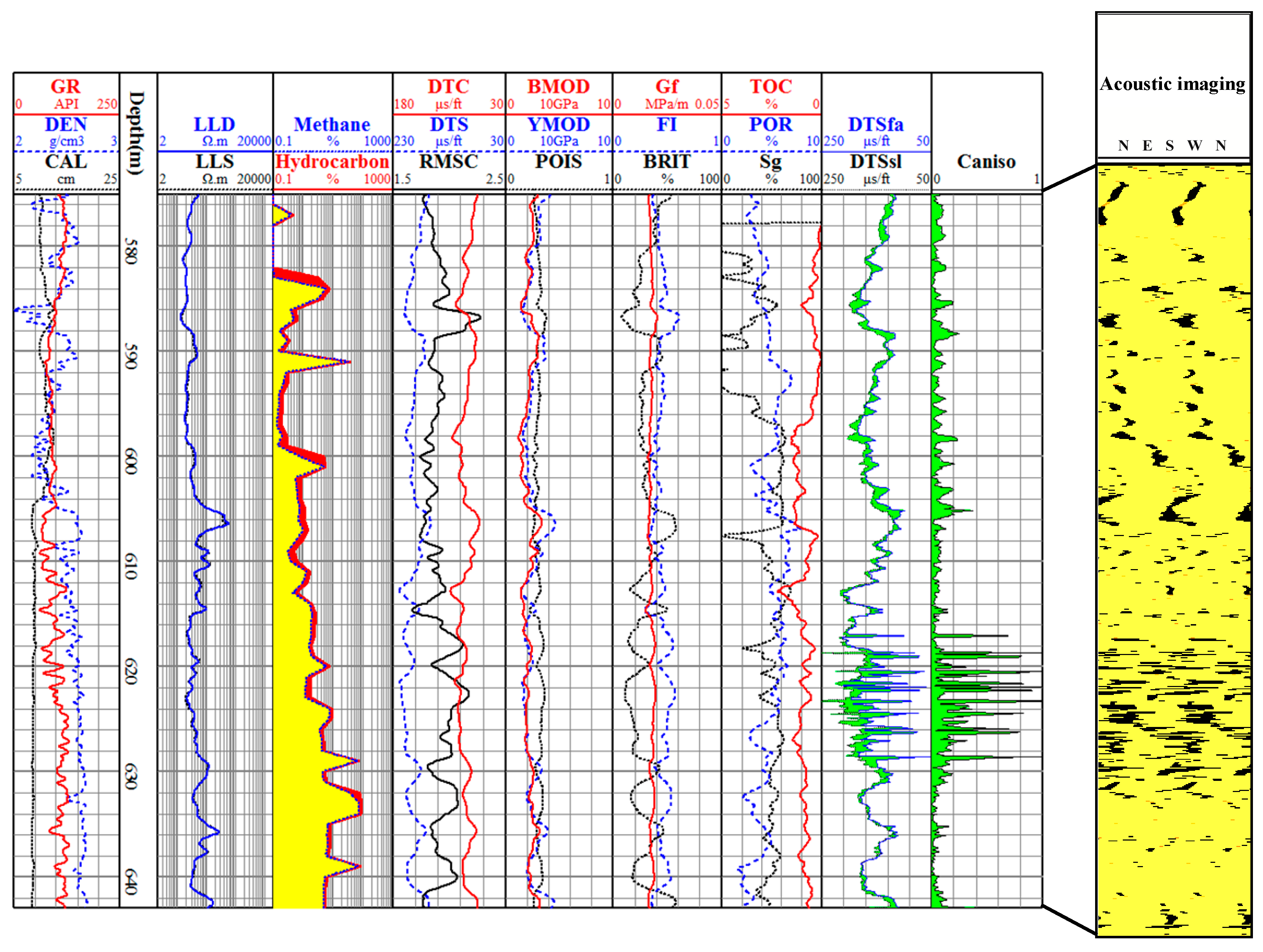
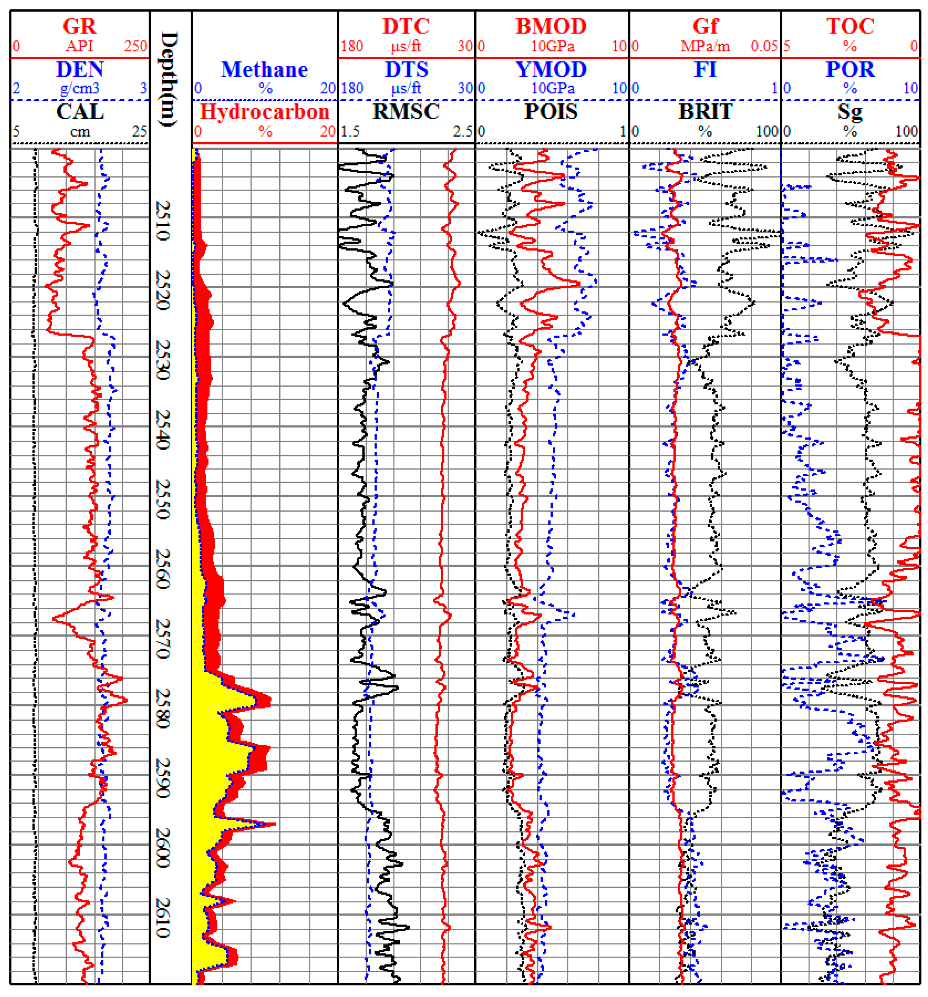
3.1. Case 1: Well A in JN Structure in the Western Hubei and Eastern Chongqing Area

The JN structure in the Western Hubei and Eastern Chongqing area is located in the center of the Shizhu synclinorium in the middle Yangtze region in the Sichuan Basin, which is one of the favorable exploration areas in the middle Yangtze. The primary target interval of the shale gas reservoirs in the JN structure is the Dongyuemiao Member of the Ziliujing Formation in the Lower Jurassic, which is dominated by shore-shallow and lacustrine-shallow lacustrine deposits with obvious hydrocarbon contents shown by gas logging in the shale zones of several wells. The TOC in this member is generally 1.0%–1.2%, and the vitrinite reflectivity (R_o) is generally 0.8%–1.5%, which suggests the presence of unconventional shale gas reservoirs.

Well A is a test well in the area that was used for the purpose of exploring continental shale gas. In the Dongyuemiao Member at 580.5–642.5 m, the lithology is dark grey and grey black shale, and gas logging shows obvious total hydrocarbon and methane contents. In the logs, the gamma ray (GR) is high, there is obvious hole enlargement (580.0–605.0 m), the DEN is around 2.30 g/cm³, the DTC in 80–90 μs/ft, the RMSC is mostly less than 2.0, and acoustic imaging reveals broken bedding, developed fine pores, and a significant anisotropy coefficient (C_aniso), which turned out to be a potential gas reservoir. In the interval of 617.0–630.0 m of the reservoir, the formation C_aniso presents several groups of spikes, showing that the micro-fractures are relatively developed, and the formation obviously contains gas (Figure 9).

In the interval of 580.5–642.5 m in Well A, the fracture pressure gradient of the reservoir was 1.60–2.00 MPa/Hm, with an average of 1.80 MPa/Hm, and the middle fracture pressure was 11.0 MPa. The frac fleet consisted of fracturing units (pumps) with a hydraulic horsepower of not less than 2000 HHP, a total hydraulic horsepower of 10,000 HHP, and an operation pressure of not less than 24 MPa. The operation pressure was shown to be more than 2.0 times that of the formation fracture pressure in this reservoir, and the fracturing equipment was able to provide a sufficient operating pressure for fracturing. In the reservoir, the POIS was an average of 0.32, the YMOD was an average of 2.5 × 10 GPa (10⁴ MPa), the BRIT was an average of 30.2, the maximum principal stress was 16.5 MPa, the minimum principal stress was 11.9 MPa, and the ΔK_i was 0.39. The fracturing stimulation was able to create multiple fractures (Figure 6 and Figure 8). A stable production level of 2100–3900 m³/d was achieved by the gas test after fracturing treatment.

3.2. Case 2: Well B in JSB Structure in the Southeastern Sichuan Area

The JSB structure in the Southeastern Sichuan area is located in the middle Yangtze region of the Sichuan Basin in China, which is a faulted anticline. It is surrounded by faults, with its major structure being gentle and the buried depth being high in its northeast and low in its southwest. The primary target interval of the shale gas reservoirs in the JSB structure mainly consists of the Longmaxi Formation of Lower Silurian—the Wufeng Formation of Upper Ordovician, which is of deep-water shelf facies sedimentation. The average TOC is more than 2.0%, the organic matter is of type Ⅰ and type Ⅱ₁, and the R_o is 2.2%–3.1%, averaging at 2.6% in the reservoirs, which are in the favorable gas generation stage and in the favorable shale gas-enriched exploration area.

Well B is a horizontal well for the exploration of marine shale gas in this area. The horizontal section in the Longmaxi Formation is at 2500.0–3767.0 m, the vertical thickness of the shale is 75 m, and its vertical depth is 2400 m, with the obvious abnormal hydrocarbon show and lithological combination of grey and dark grey shale and grey black carbonaceous shale. The GR shows high values of 130–180 API; the DEN is about 2.60 g/cm³; and the RMSC is less than 1.8 (Figure 10). Its total porosity is 1.3%–9.8%, averaging at 4.5%, and its gas saturation is 25%–84%, averaging at 58.0%.

In the horizontal interval of 2500.0–3767.0 m in Well B, the fracture pressure gradient was found to be 1.40–1.60 MPa/Hm, with an average of 1.50 MPa/Hm, and the fracture pressure was 36.0 MPa. The frac fleet consisted of fracturing units (pumps) with a hydraulic horsepower of not less than 2500 HHP, a total hydraulic horsepower of 40,000 HHP, and an operation pressure of not less than 70 MPa. The operation pressure was shown to be more than 1.5 times that of the formation fracture pressure in this reservoir, and the fracturing equipment was able to provide sufficient operating pressure for fracturing. The POIS was an average of 0.24, the YMOD was an average of 4.8 × 10 GPa (10⁴ MPa), the BRIT was an average of 59.1, the maximum principal stress was 63.50 MPa, the minimum principal stress was 47.39 MPa, and the ΔK_i was 0.34. The fracturing stimulation was able to create radial fracture networks (Figure 6 and Figure 8). A stable production of 20.3 × 10⁴ m³/d was achieved by the gas test after 15 stages of frac.

4. Discussion

Compared with conventional acoustic logging, dipole array acoustic logging has more abundant formation information, which expands the application scope of acoustic logging data. Dipole array acoustic logging data can be used to identify the formation lithology, gas potential, and fractures, and has obvious advantages in terms of the reservoir stimulation potential. It can provide rock mechanical data such as the Poisson’s ratio, Young’s modulus, and fracture index, and can deliver critical support for optimizing the development plans of oil and gas wells and selecting a drilling fluid density for safe drilling, which is not subjected to replacement by the conventional logging method.

Although dipole array acoustic logging is widely used for reservoir evaluation, there are some ambiguities in the use of individual logging data to evaluate some indicators of the formation; the same as for the dipole array acoustic logging data. In the logging evaluation of reservoirs under complex geological conditions, the borehole environment interference should be eliminated, and the main formation characteristics should be highlighted. It is also best to verify with various logging data as much as possible. It has been found that the combination of dipole array acoustic logging data with the hydrocarbon content from gas logging data can improve the accuracy and reliability of reservoir evaluation. Combined with electrical imaging logging data, fractures can be evaluated more accurately, and combined with nuclear magnetic resonance (NMR) logging data, reservoir parameters such as saturation and permeability can be calculated more accurately. Therefore, when the dipole array acoustic logging data is used, especially for the reservoir evaluation of shale gas reservoirs, more relevant data should be combined to ensure the accuracy and reliability of the evaluation results.

In addition, the porosity and saturation methods given in this paper are empirical formulas based on the analysis of logging measured data. In the future, it is necessary to use rock physics and geological mathematics to deeply study the mechanism and related basic theory involved in the formation of such reasonable phenomena. For example, the reservoir parameters should be studied using classical density functional theory [49].

5. Conclusions

This paper describes the application of dipole array acoustic logging in shale gas reservoir evaluation and verified this method using typical shale gas wells in two blocks in the Sichuan Basin. The findings of this paper can be summarized as follows:

(1)

The dipole array acoustic logging data can be used to effectively evaluate the lithology, gas potential, and stimulation potential in shale gas reservoirs. The dipole S-wave anisotropy coefficient variation characteristics can be used to accurately determine the effectiveness of fractures in shale gas reservoirs.

(2)

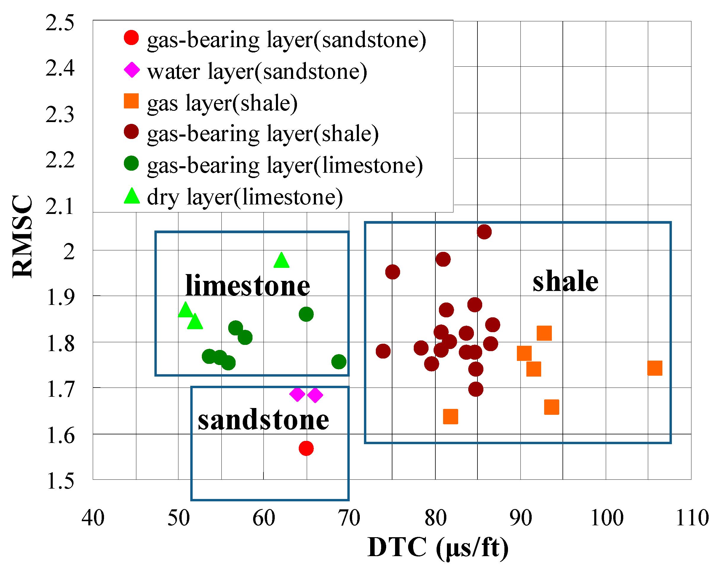
When shale reservoirs contain gas, the RMSC will be significantly reduced, usually to less than 2.00, and that of the typical shale gas reservoirs will be less than 1.80; the RMSC of the reservoir is combined with the hydrocarbon content from gas logging data to more effectively identify the gas potential of shale reservoirs.

(3)

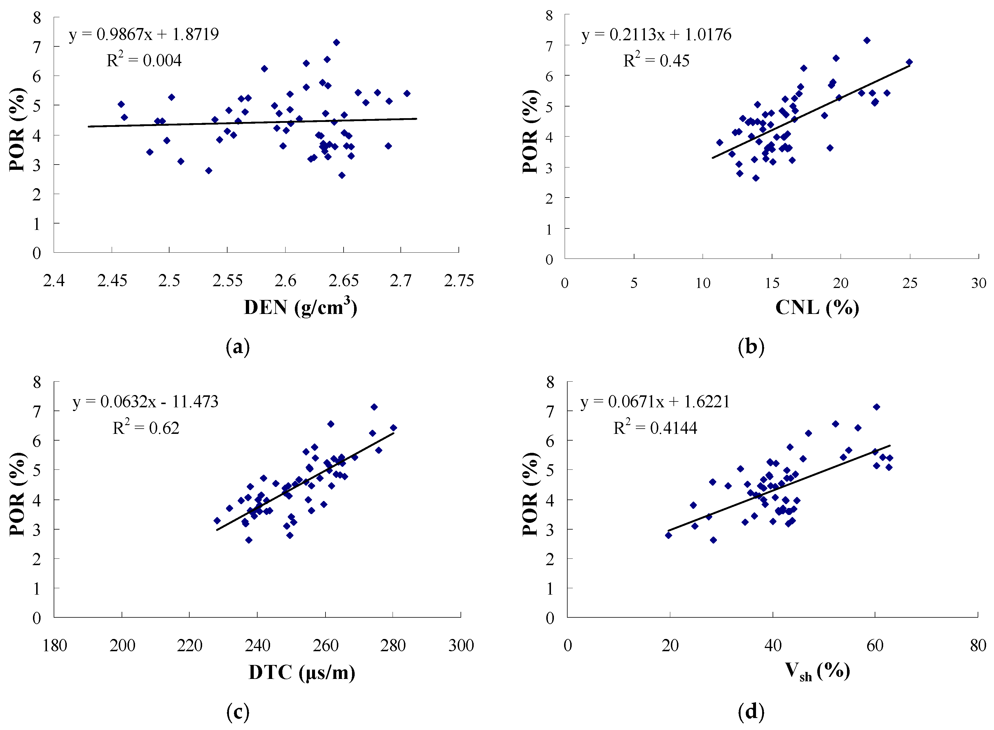
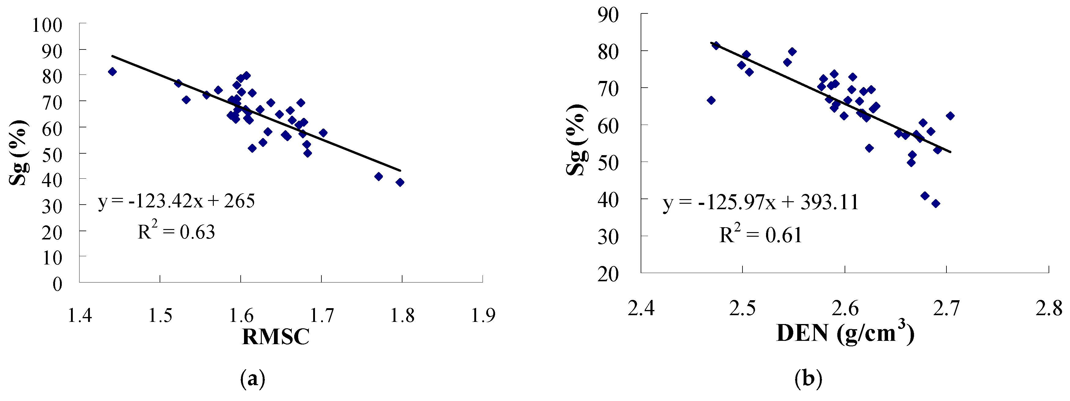
By using the relationship between the DTC and total porosity of the shale gas reservoir, the total porosity of the shale gas reservoir can be accurately calculated combined with the CNL and V_sh of the reservoir; the gas saturation of the shale gas reservoir can be calculated by using the RMSC and DEN, which innovatively extends the application of data.

(4)

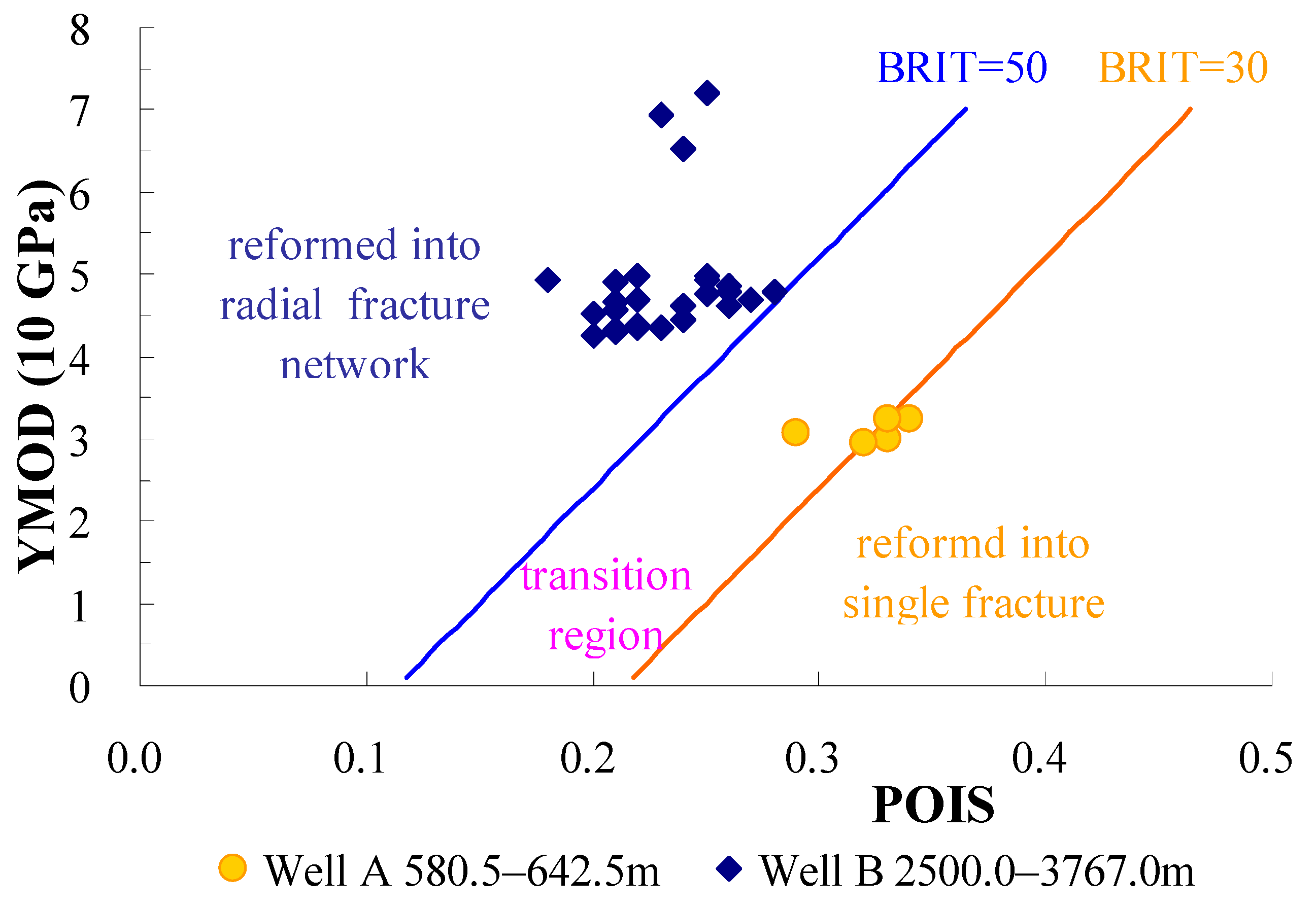
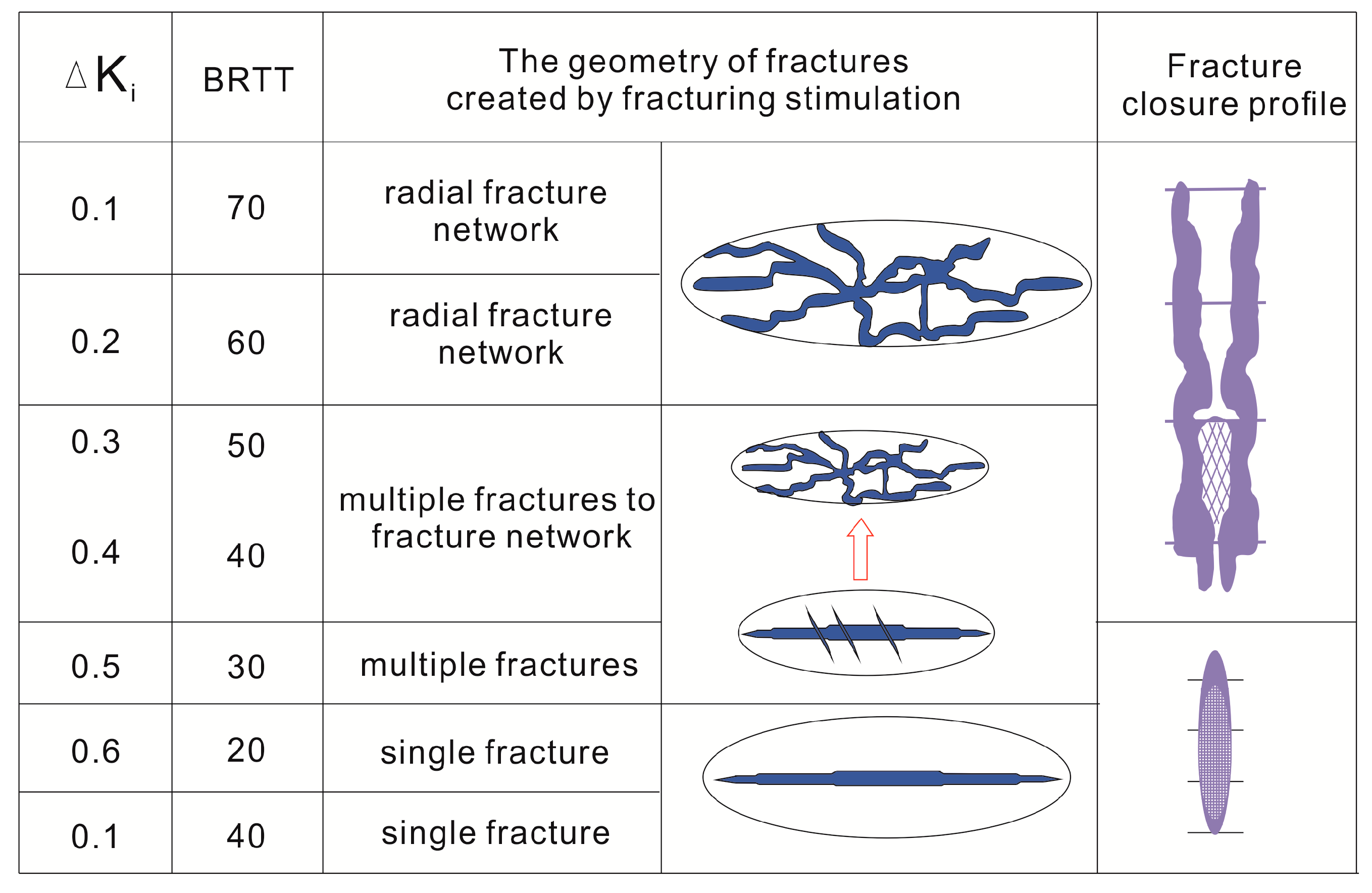
For the stimulation potential of shale gas reservoirs, the fracture shapes resulting from frac stimulation can be more accurately evaluated in combination with BRIT and ΔK_i. If the conditions of BRIT ≥ 50 and ΔK_i ≤ 0.3 are usually fulfilled, stimulation of the reservoir tends to form the radial fracture network.

(5)

Calculation of the fracture pressure gradient of shale gas reservoirs by the improved Eaton model is more accurate, and evaluation of the formation fracture pressure can provide guideline for the fracturing of shale gas reservoirs.

6. Patents

Equation 10 is derived from the Chinese invention patent ”Mud logging method for formation fracture pressure gradient in shale gas reservoir” filed by the authors’ team. The number of this patent is 201410123365.3, which was authorized on 12 April 2017.

References

1. Jarvie, D.M.; Hill, R.J.; Ruble, T.E.; Pollastro, R.M. Unconventional shale-gas systems: The Mississippian Barnett Shale of north-central Texas as one model for thermogenic shale-gas assessment. AAPG Bull. 2007, 91, 475–499. [Google Scholar] [CrossRef]
2. Cao, H.; Wang, T.Y.; Bao, T.; Sun, P.H.; Zhang, Z.; Wu, J.J. Effective exploitation potential of shale gas from Lower Cambrian Niutitang Formation, Northwestern Hunan, China. Energies 2018, 11, 3373. [Google Scholar] [CrossRef]
3. Shi, W.R.; Wang, X.Z.; Zhang, C.M.; Feng, A.G.; Huang, Z.S. Experimental study on gas content of adsorption and desorption in Fuling shale gas field. J. Petrol. Sci. Eng. 2019, 180, 1069–1076. [Google Scholar] [CrossRef]
4. Zou, C.N.; Dong, D.Z.; Wang, Y.M.; Li, X.J.; Huang, J.L.; Wang, S.F.; Guan, Q.H.; Zhang, C.C.; Wang, H.Y.; Liu, H.L.; et al. Shale gas in China: Characteristics, challenges and prospects (II). Petrol. Explor. Dev. 2016, 43, 182–196. [Google Scholar] [CrossRef]
5. Li, Y.X.; Qiao, D.W.; Jiang, W.L.; Zhang, C.H. Gas content of gas-bearing shale and its geological evaluation summary. Geol. Bull. Chin. 2011, 30, 308–317. [Google Scholar]
6. Glorioso, J.C.; Rattia, A. Unconventional reservoirs: Basic petrophysical concepts for shale gas. In Proceedings of the SPE/EAGE European Unconventional Resources Conference and Exhibition, Vienna, Austria, 20–22 March 2012. [Google Scholar] [CrossRef]
7. Zou, C.N.; Dong, D.Z.; Yang, Y.; Wang, Y.M.; Huang, J.L.; Wang, S.F.; Fu, C.X. Conditions of shale gas accumulation and exploration practices in China. Nat. Gas. Ind. 2011, 31, 26–39. [Google Scholar] [CrossRef]
8. Lucier, A.M.; Hofmann, R.; Bryndzia, L.T. Evaluation of variable gas saturation on acoustic log data from the Haynesville Shale Gas Play, NW Louisiana, USA. Lead. Edge 2011, 30, 300–311. [Google Scholar] [CrossRef]
9. Qi, Q.M.; Muller, T.M.; Pervukhina, M. Sonic QP/QS ratio as diagnostic tool for shale gas saturation. Geophysics 2017, 82, 97–103. [Google Scholar] [CrossRef]
10. Wu, X.G.; Ji, F.L.; Li, D.C. Application status and research progress of dipole acoustic well logging. Prog. Geophys. 2016, 31, 380–389. [Google Scholar] [CrossRef]
11. Fan, Z.Y.; Hou, J.G.; Ge, X.M.; Zhao, P.Q.; Liu, J.Y. Investigating influential factors of the gas absorption capacity in shale reservoirs using integrated petrophysical, mineralogical and geochemical experiments: A case study. Energies 2018, 11, 3078. [Google Scholar] [CrossRef]
12. Ma, Y.S.; Cai, X.Y.; Zhao, P.R. China’s shale gas exploration and development: Understanding and practice. Petrol. Explor. Dev. 2018, 45, 561–574. [Google Scholar] [CrossRef]
13. Tang, X.M.; Chunduru, R.K. Simultaneous inversion of formation shear-wave anisotropy parameters from cross-dipole acoustic-array waveform data. Geophysics 1999, 64, 1502–1511. [Google Scholar] [CrossRef]
14. Sinha, B.K. Stress-induced azimuthal anisotropy in borehole flexural waves. Geophysics 1996, 61, 1899–1907. [Google Scholar] [CrossRef]
15. Tang, X.M.; Cheng, C.H. Quantitative Borehole Acoustic Methods; Elsevier Science Publishing: Berlin, Germany, 2004. [Google Scholar]
16. Kessler, C.; Varsamis, G.L. A New Generation Crossed Dipole Logging Tool: Design and Case Histories. In Proceedings of the SPE Annual Technical Conference and Exhibition, New Orleans, LA, USA, 30 September–3 October 2001. [Google Scholar] [CrossRef]
17. Xiang, M.; Wang, Z.W.; Liu, J. Extracting array acoustic logging signal information by combining fractional fourier transform and Choi–Williams distribution. Appl. Acoust. 2015, 90, 111–115. [Google Scholar] [CrossRef]
18. Li, Y.X.; Li, Y.M. Multipole acoustic array logging tool. Well Log. Technol. 2008, 32, 439–442. [Google Scholar]
19. Sima, L.Q. Logging Evaluation Method and Application of Carbonate Reservoir; Petroleum Industry Press: Beijing, China, 2009. (In Chinese) [Google Scholar]
20. Zhang, C.G.; Xiao, C.W.; Li, W.Y. Study on Acoustic Full Waveform Logging Response Characteristics and Its Application Interpretation; Hubei Science and Technology Press: Wuhan, China, 2008. (In Chinese) [Google Scholar]
21. Zhang, J.Z. Relationship among P-S wave velocity ratio matrix lithology exponent and porosity exponent. J. Xinan Petrol. Inst. 1990, 5, 89–91. [Google Scholar]
22. Koesoemadinata, A.P.; Mcmechan, G.A. Empirical estimation of viscoelastic seismic parameters from petrophysical properties of sandstone. Geophysics 2001, 66, 1457–1470. [Google Scholar] [CrossRef]
23. Guerin, G.; Goldberg, D. Sonic waveform attenuation in gas hydrate-bearing sediments from the Mallik 2l-38 research well, Mackenzie Delta, Canada. J. Geophys. Res. Sol. Earth 2002, 107, 1–11. [Google Scholar] [CrossRef]
24. Klimentos, T. Attenuation of P-and S-waves as a method of distinguishing gas and condensate from oil and water. Geophysics 1995, 60, 447–458. [Google Scholar] [CrossRef]
25. Zeng, W.C.; Qiu, X.B.; Liu, X.F. A new method to identify fluid properties in complex reservoir. Well Log. Technol. 2014, 38, 11–21. [Google Scholar]
26. Gassmann, F. Elastic waves through a packing of spheres. Geophysics 1951, 16, 673–682. [Google Scholar] [CrossRef]
27. Zhao, J.H.; Jin, Z.J.; Jin, Z.K.; Hu, Q.H.; Hu, Z.Q.; Du, W. Mineral types and organic matters of the Ordovician-Silurian Wufeng and Longmaxi Shale in the Sichuan Basin, China: Implications for pore systems, diagenetic pathways, and reservoir quality in fine-grained sedimentary rocks. Mar. Petrol. Geol. 2017, 86, 655–674. [Google Scholar] [CrossRef]
28. Xu, Z.; Shi, W.Z.; Zhai, G.Y.; Bao, S.J.; Peng, N.J.; Zhang, X.M.; Wang, C.; Xu, H.Q.; Wang, R. Well logging prediction for total porosity of shale in Fuling area. Acta Pet. Sin. 2017, 38, 533–543. [Google Scholar] [CrossRef]
29. Archie, G.E. The electrical resistivity log as an aid in determining some reservoir characteristics. Trans. AIME 1942, 146, 54–62. [Google Scholar] [CrossRef]
30. Simandoux, P. Dielectric measurements on porous media, application to the measurement of water saturation: Study of the behavior of argillaceous formations. Rev. Inst. Fr. Pet. 1963, 18, 193–215. [Google Scholar]
31. Poupon, A.; Leveaux, J. Evaluation of water saturations in shaly formations. In Proceedings of the SPWLA 12th Annual Logging Symposium, Dallas, TX, USA, 2–5 May 1971. [Google Scholar]
32. Schlumberger. Log Interpretation Volume 1: Principles; Schlumberger Education Services: Paris, France, 1972. [Google Scholar]
33. Boyce, M.L.; Carr, T.R. Lithostratigraphy and petrophysics of the Devonian Marcellus Interval in West Virginia and Southwestern Pennsylvania. GCSSEPM Proc. 2009, 10, 254–281. [Google Scholar] [CrossRef]
34. Shi, W.R.; Zhang, Z.S.; Zhang, J.P.; Zhao, H.Y.; Shi, Y.H.; Huang, Q. Conventional well logging interpretation model for shale gas in Dongyuemiao Member of Jiannan area: An example from JYHF-1 Well. Nat. Gas. Explor. Dev. 2014, 37, 29–34. [Google Scholar] [CrossRef]
35. Zheng, Y.B.; Tang, X.M.; Patterson, D.J. Identifying stress-induced anisotropy and stress direction using cross-dipole acoustic logging. In Proceedings of the SPWLA 50th Annual Logging Symposium, Woodlands, TX, USA, 21–23 June 2009. [Google Scholar]
36. Tang, X.M.; Patterson, D. S-wave anisotropy measurement using cross-dipole acoustic logging: An overview. Petrophysics 2001, 42, 107–117. [Google Scholar]
37. Rickman, R.; Mullen, M.; Petre, E.; Grieser, B.; Kundert, D. A practical use of shale petrophysics for stimulation design optimization: All shale plays are not clones of the Barnett Shale. In Proceedings of the SPE Annual Technical Conference and Exhibition, Denver, CO, USA, 21–24 September 2008. [Google Scholar] [CrossRef]
38. Grieser, B.; Bray, J. Identification of production potential in unconventional reservoirs. In Proceedings of the SPE Production and Operations Symposium, Oklahoma City, OK, USA, 31 March–3 April 2007. [Google Scholar] [CrossRef]
39. Shi, X.; Wang, J.; Ge, X.M.; Han, Z.Y.; Qu, G.Z.; Jiang, S. A new method for rock brittleness evaluation in tight oil formation from conventional logs and petrophysical data. J. Petrol. Sci. Eng. 2017, 151, 169–182. [Google Scholar] [CrossRef]
40. Jin, X.C.; Shah, S.N.; Roegiers, J.C.; Zhang, B. An integrated petrophysics and geomechanics approach for fracability evaluation in shale gas reservoirs. SPE J. 2015, 7, 518–526. [Google Scholar] [CrossRef]
41. Olson, J.E.; Taleghani, A.D. Modeling simultaneous growth of multiple hydraulic fractures and their interaction with natural fractures. In Proceedings of the SPE Hydraulic Fracturing Technology Conference, Woodlands, TX, USA, 19–21 January 2009. [Google Scholar] [CrossRef]
42. He, J.M.; Zhang, Z.B.; Li, X. Numerical analysis on the formation of fracture network during the hydraulic fracturing of shale with pre-existing fractures. Energies 2017, 10, 736. [Google Scholar] [CrossRef]
43. Zhou, H.; Meng, F.Z.; Zhang, C.Q.; Xu, R.C.; Lu, J.J. Quantitative evaluation of rock brittleness based on stress-strain curve. Chin. J. Rock Mech. Eng. 2014, 6, 1114–1122. [Google Scholar] [CrossRef]
44. Qi, Q. Application of in-suit stress prediction technology in shale gas horizontal wells development. Prog. Geophys. 2018, 33, 1117–1122. [Google Scholar] [CrossRef]
45. Eaton, B.A. Fracture gradient prediction and its application in oilfield operations. J. Petrol. Technol. 1969, 21, 1353–1360. [Google Scholar] [CrossRef]
46. Zhang, J.P.; Feng, A.G.; Shi, Y.H.; Zhao, H.Y.; Xiao, S.K.; Ren, Y.; Shi, W.R.; Li, G.H.; Tian, F. Mud Logging Method for Formation Fracture Pressure Gradient in Shale Gas Reservoir. China Patent 201410123365.3, 12 April 2017. [Google Scholar]
47. Cipolla, C.L.; Warpinski, N.R.; Mayerhofer, M.J.; Lolon, E.P.; Vincent, M.C. The relationship between fracture complexity, reservoir properties, and fracture treatment design. In Proceedings of the SPE Annual Technical Conference and Exhibition, Denver, CO, USA, 21–24 September 2008. [Google Scholar] [CrossRef]
48. Cipolla, C.L.; Lolon, E.P.; Dzubin, B. Evaluating stimulation effectiveness in unconventional gas reservoirs. In Proceedings of the SPE Annual Technical Conference and Exhibition, New Orleans, LA, USA, 4–7 October 2009. [Google Scholar] [CrossRef]
49. Lee, J.W.; Nilson, R.H.; Templeton, J.A.; Griffiths, S.K.; Kung, A.; Wong, B.M. Comparison of molecular dynamics with classical density functional and Poisson−Boltzmann theories of the electric double layer in nanochannels. J. Chem. Theory Comput. 2012, 8, 2012–2022. [Google Scholar] [CrossRef]
Figure 1. Structural schematic for the acoustic system of the dipole array acoustic logging tool.
Energies 12 03882 g001
Figure 2. The plot for RMSCs of different types of reservoirs in some block of China (data from the south Sichuan area of Sichuan Basin, provided by the laboratory of Sinopec Oilfield Service Corporation).
Energies 12 03882 g002
Figure 3. Relationship between the core porosity and logging parameters of the Longmaxi–Wufeng Formation shale in the Sichuan Basin: (a) correlation between the core porosity and the DEN; (b) correlation between the core porosity and the CNL; (c) correlation between the core porosity and the DTC; (d) correlation between the core porosity and the Vsh.
Energies 12 03882 g003
Figure 4. Relationship between the core gas saturation and logging parameters of the Longmaxi–Wufeng Formation shale in the Sichuan Basin: (a) correlation between core gas saturation and RMSC; (b) correlation between core gas saturation and DEN.
Energies 12 03882 g004
Figure 5. Schematic diagram for cross-dipole array acoustic logging in the anisotropic formation.
Energies 12 03882 g005
Figure 6. The POIS–YMOD evaluation plot for stimulated fractures in shale gas reservoirs.
Energies 12 03882 g006
Figure 7. Comparison of calculation results of fracture pressure models with the measured fracture pressure of shale gas wells in Sichuan Basin.
Energies 12 03882 g007
Figure 8. The diagram for the fracture forming conditions for the stimulation of a gas reservoir [37,44].
Energies 12 03882 g008
Figure 9. The presentation log of rock mechanics and dipole array acoustic anisotropy in Well A.
Energies 12 03882 g009
Figure 10. The presentation log for rock mechanics in the horizontal section (2500.0–2620.0 m) of Well B.
Energies 12 03882 g010